Object-oriented sub-zonal modelling for efficient energy-related building simulation

Abstract

When modelling and simulating a building to evaluate its energy-related performance, reproducing the behaviour of the contained air volumes is very important. For that purpose, fully mixed models (i.e. for instance, a single temperature per room) easily prove inadequate, while computational fluid dynamics ones do not provide sufficient simulation speed, and are difficult to formulate and manage in a modular manner. This manuscript presents a somehow intermediate solution based on the object-oriented modelling paradigm, and implemented in the Modelica language. The proposal advantages are illustrated by two significant examples.

Keywords:

• building simulation
• energy optimization
• object-oriented modelling

1. Introduction and research motivation

Modelling and simulation of dynamic systems is very important for optimizing the energy efficiency of buildings [1–3]. In this field, a primary challenge is to effectively confront the inherently multi-physic nature of the problem [4]. The energy performance of a building results from heterogeneous phenomena (hydraulic, thermal, electric and so forth) and the operation of several control systems and the actions of the inhabitants. More precisely, energy performance is determined by the interaction of all those phenomena [5], which further complicates the scenario. Virtually the totality of engineering tools – and design practices – broadly distinguish (a) the ‘building’ stricto sensu, that is, walls, doors, windows; (b) the contained air volumes, possibly divided in zones; (c) the heating, ventilation and air conditioning (HVAC) system; (d) automation and control systems; and (e) energy sources/sinks owing to the building utilization, for example, the heat released by occupants, industrial machines or whatever is installed. The subsystems' interaction is accounted for by having some of them provide boundary conditions for some others. This is quite far from an integrated approach, but tools that address the simulation of all (or at least part) of the subsystems in a coordinated way are at present little more than research objects [5–7].

The main reason for such a scenario is the very different issues posed by the various subsystems. For example, control system models are made of oriented blocks and may need a continuous-time or a digital representation depending on the simulation purpose; HVAC models, conversely, live invariantly in the continuous-time domain, but are typically 0- or 1D, while models of phenomena that occur in continua such as a wall or an air volume often cannot avoid 3D distributions. As a result, it is difficult to devise models that address all the necessary phenomena, and can be organized in a modular way to the advantage of their construction, parametrization and maintenance. To witness that, it is enough to throw a glance at the building-related literature on ‘whole building simulation’: methodological and engineering issues are discussed, for example, in [8,9] and the papers quoted therein, while the encountered difficulties are well evidenced by works such as [10–13].

This work concentrates on a major source of the mentioned problem, that is the modelling of air volumes. Specifically, this research exploits the fact that whole buildings models are of interest for system level studies, where one can sacrifice detailed descriptions (e.g. of an air velocity field) in exchange for a correct representation of how all the phenomena interact to produce the main energy outcome: in some sense, although this is not the most correct definition from a theoretical standpoint, in system level simulation one is interested in realistically reproducing ‘what would be seen by a control and supervision system’. Based on the consideration above, an efficient compromise can be devised between models based on the simple and efficient (but often too imprecise) ‘fully mixed’ paradigm, where air conditions in each volume are assumed uniform, and models based on the complex (but accurate) fine-scale 3D computational fluid dynamics (CFD) one. This work presents a modelling approach aimed at said compromise, and a proof of concept for its validity.

2. Contribution and related work

A widely used paradigm in the addressed modelling context is that of zonal models or zoning, where the air within a building is split into zones, typically corresponding, for example, to rooms. Zones are therefore macro-volumes with respect to the scale of the spatial temperature and flow distribution. This allows for a small number of variables, that characterize ‘storage' elements, devoted to mass and energy balances, and ‘flow’ elements, that describe the mass and energy flow among the storages. As a result, zonal models are naturally modular – for example, they are often given electric network equivalents – and computationally simple. However, they pose non-trivial problems as for the way to compute average air properties in the zones, to the detriment of both accuracy and simulation results’ interpretability. Nonetheless, for efficiency reasons, much literature work and many engineering tools adopt the zonal approach: for example, COMIS, CONTAM, POMA, see [14–17], and EnergyPlus [18].

On the opposite side with respect to zoning stands, fine-scale 3D CFD that provides far higher accuracy, but apart from complexity, has a significant drawback: it is not immediate to separate the (partial) differential equations that hold within a volume from the boundary conditions. The creation of modular models is thus a complex task, and in some cases virtually impossible if not at the cost of an extremely cumbersome and redundant software implementation. There exist 3D CFD tools which can be applied to buildings, for example, Fluent [19,20], but they are hardly ever considered in system level studies.

In recent years, object-oriented modelling (OOM) has emerged as a promising tool to effectively balance accuracy, efficiency and modularity (see e.g. [21]). OOM fosters modularity via a clear separation of the behaviour of a component (roughly, its constitutive equations) from its interface, that is the variables that – once related by suitable connection equations to variables of other components – yield the overall aggregate model. A first important step in this direction is [22], where the idea of zonal modelling is integrated in the OOM language Modelica [23]. In [24], a comparison between Modelica models and TRNSYS (a major software product for thermal analysis and certification) is reported. The authors state that they have obtained ‘a five-to tenfold reduction in model development time by using the equation-based model representation language Modelica compared to the time that was required to implement a model with similar physics in C/C++' and that they ‘expect that a similar comparison holds between Modelica and TRNSYS, but cannot provide data on this comparison because TRNSYS’ building model evolved over several years which makes a time estimate difficult if not impossible’. In any case, their experience with Modelica ‘is that it is easier in Modelica to construct large models than it is in TRNSYS’. In general, based on our experience, we can thus say that Modelica yields comparable results with respect to other environments, with less human effort. Incidentally, in [24] an extensive comparison between Modelica and TRNSYS models is quoted, see [25]. The interest for Modelica is further evidenced by other papers such as [26] and [27], which is somehow an ancestor of this work, but sticks to the fully mixed approach although envisaging the necessity of extensions.

To date, in fact, OOM-related research enforces modularity by relying on the zonal models idea, which is the easiest way to go, but definitely not the most accurate. In the last years a somehow intermediate proposal, termed sub-zonal modelling or sub-zoning, was formulated. The basic idea behind sub-zoning is to set up zonal models that allow to split particular zones with a finer discretization [28–30]. This improves accuracy at the cost of a (moderate) complexity increase, but still poses non-trivial issues with respect to modularity, especially if air models need to be connected to heterogeneous entities such as prescribed boundary conditions (e.g. from the external environment), walls, piping and so on.

This work, that is part of a long-term research aimed specifically at system level building simulation models, aims at filling the gap just sketched, and its contribution can be summarized as follows: First, for the problem of modelling air volumes, a particular spatial discretization of the Navier–Stokes momentum equations is proposed. Notice that most of the literature adopting the finite volume approach, which is almost inherent to zoning, simply do not introduce that equation explicitly. Also, specific simplifications are introduced for the addressed domain (e.g. ‘low’ air velocities are assumed). These approximations reduce the model nonlinearity, facilitating its numerical solution. Of course accuracy suffers in the description of highly local and directional phenomena like jets and plumes, but since the goal of the overall research not to capture such details, the said inaccuracy is largely acceptable (see also the examples reported later on). From this point of view, the presented research can help solve problems like those mentioned in [31], where a real-time capable air flow model was required, and a (coarser) Modelica implementation did not prove successful.

The scope of the obtained models is thus limited to air volumes in buildings or similar situations, where a fully mixed approach would be too inaccurate (e.g. for the relevance of vertical stratification or more in general of temperature difference in large structures such as factories, gyms, hotel lobbies, fair pavilions and so forth) but simulation efficiency is an issue. Second, it is shown that the proposed approach, declined in the OOM framework, allows to obtain modular models, with a scalable level of complexity – for example, for turbulence descriptions. Standardized, uniform interfaces allow an easy integration of the obtained models with 0- or 1D ones (e.g. for HVAC piping) and heterogeneous elements (e.g. industrial machines or household appliances releasing power to the air). Care is taken to reduce the number of empirical parameters to a minimum: for example, a simplified (yet well assessed) turbulence model is used. From this point of view, then, the scope of the proposed models is basically (but not only) efficient whole-building simulation, in a specific view to control and optimize, based on realistically available data (also for existing buildings).

Models are realized in the Modelica language [23,32,33] and totally integrated with the Modelica standard libraries, allowing to avoid co-simulation in favour of an efficient and user-friendly solution. Examples show that the obtained results are in reasonable accordance with those of fine-scale 3D CFD models (of course, as long as the introduced simplifications are valid), while the simulation speed is significantly higher. In addition, although the matter is not treated in this manuscript, the standardized interface allows to couple the obtained models with others, also from different physical domains, in a very straightforward manner. For all the reasons above, the authors consider this manuscript a step forward in the direction of a really integrated paradigm for building modelling.

3. The proposed modelling approach

3.1. Balance equations

We start from the mass, energy balance and the Navier–Stokes (momentum) equations, that for the purpose of this work can be written as

(1)

(2)

(3)

where the scalars p, T, e, h and ρ are, respectively, the fluid pressure, temperature, specific energy, specific enthalpy and density, the vectors v and f _T are the fluid velocity and the resultant of all the acting forces, both external like gravity and internal like friction, and the scalar parameter k is the fluid thermal conductivity. In the following, Equations (1)(1) (2)–(3)(3) are spatially discretized with reference to finite volume elements (not necessary uniform) of parallelepiped shape, A_{x ,y,z} being the areas of the element faces normal to the x-, y- and z-axes, and V the element volume. The mass and energy equations are treated in quite standard a manner, giving rise to the two scalar ones:

(4)

(5)

where are the mass flow rates across the two surfaces orthogonal to axis a, assumed positive when entering the element, are the specific enthalpies transported by fluid motion across said surfaces, the thermal powers crossing the same surfaces without fluid motion (due to, e.g. diffusion), and Q_g the thermal power possibly generated within the volume.

Also the finite-volume discretization of the mass and energy equation is totally standard, it is thus not described for brevity. However, as anticipated, the spatial discretization adopted here for the momentum equation is novel, introducing an ad hoc approximation for the velocities' second derivatives, and a corresponding treatment of the boundary volume elements.

First, the Newtonian fluid simplification is adopted, thereby rewriting Equation (3)(3) as

(6)

where μ is the fluid dynamic viscosity, and f represents the external forces only, such as gravity. The scalar projection is then brought in. This yields the three scalar equations

(7)

(8)

(9)

where the subscripts x, y and z denote the axes. In the case of natural convection having as vertical axis the z one, clearly f_x  = f_y  = 0 and f_z  = –ρg, where g is the gravity acceleration. The convective term ∇·(ρvv ^T ) is neglected here, since its relevance is small when dealing with such low velocities as those of airflows in building rooms. Also, only the component of air velocities orthogonal to the volume surfaces are considered, leading de facto to a ‘quasi-3D’ modelling approach. Summing up, after the mentioned manipulations, the equations to be discretized are

(10)

(11)

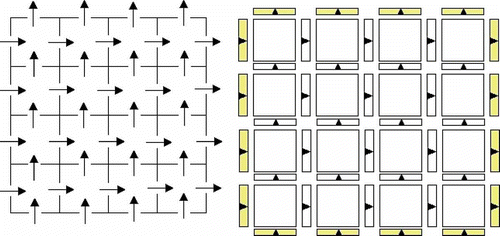
Spatial discretization is managed as described in the following, referring to the 2D case with the x and z (vertical) axes only (the 3D extension is trivial and would only unnecessarily complicate the notation). A staggered grid of points [34,35] is defined in the spatial domain of interest, as illustrated in Figure 1(a). Some of the nodes are attributed to control volumes, to which the mass and energy equations are referred. Some other nodes are conversely relative to the fluid motion among said volumes, thus being the locations to which velocities are attributed. In a parallelepiped-based grid the two sets of nodes form a ‘staggered’ pattern, whence the name.

Figure 1. Staggered grid (a) evidencing pressure and velocities nodes, and grid application to the (b) x and (c) z momentum equations.

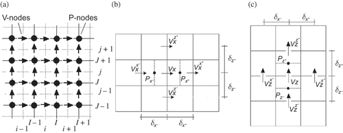
For the discretization of the x- and z-axis momentum Equations (10)(10) and (11) the grid of Figure 1(b) and (c) is considered, and in this treatise the only moving force introduced is gravity (directed as the negative z-axis); generalizations to other forces are straightforward, recall Equations (7)(7) (8)–(9)(9). In Figure 1 and the following analogous ones, arrows indicate the positive velocity direction assumed when discretizing the momentum equations.

First, consider the x equation. The velocity to be computed is V_x , while , , and denote, respectively, the x component of velocities in the ‘west’, ‘east’, ‘south’ and ‘north’ surrounding velocity nodes – a notation that Figure 1(b) should make self-explanatory. Analogously, and are the pressures of the west and east pressure nodes. The distances between the node in which the V_x velocity is computed and the surrounding ones where the x velocity components are accounted for, are denoted by , , and .

In Equation (10)(10), three terms have to be spatially discretized. The first one is ∂p/∂x, that simply yields

(12)

The second term is . Assuming the viscosity μ uniform in the volume element, one can write

(13)

For the second partial derivative of the x velocity with respect to x, a second-order polynomial function is taken as local approximant, and readily parametrized as

(14)

(15)

(16)

which is an ad hoc simplification similar to others proposed in the literature [36–38], and particularly suited for the case at hand. The required second derivative approximation is thus 2a(4), which yields

(17)

allowing to reformulate (13) as

(18)

The last term to be discretized is . Also in this case since the viscosity is assumed uniform in the element, this yields

(19)

and for the second partial derivative of the x velocity with respect to z, a second-order polynomial approximant is again taken. With a reasoning similar to that previously reported, Equation (19)(19) is thus approximated as

(20)

Considering the z momentum equation, the same approach can be followed referring to Figure 1(c), where the momentum equation is applied to velocity V_z , and , , and are the left, right, south and north surrounding z velocities; and the pressures of the adjacent south and north pressure nodes. The relevant distances are here , , and .

The only difference with respect to the x axis is the presence of gravity, and simply replicating the computational scheme above leads to

(21)

(22)

(23)

The discretized momentum equations reported so far are valid in the volumes within a cavity (a room, a duct, a box...) but apparently not for the volumes at the cavity boundaries. As shown in Figure 2(a) and (b), velocity nodes referring to volumes at the boundary may not have west/east neighbours for the x velocity case, and may not have north/south neighbours for the z case. A special momentum equation discretization is thus required for boundary velocities.

Figure 2. Boundary layer for (a) x and (b) z velocity, and grid for the (c) x momentum equation on the west boundary.

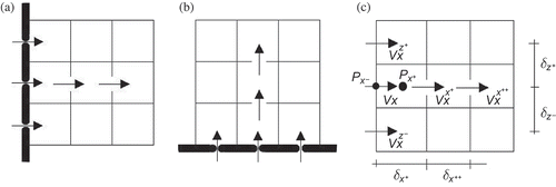
For brevity, consider the x case in a velocity node located on the west cavity boundary (the other cases are analogous) illustrated in Figure 2(c). The equation to be discretized is Equation (10)(10), requiring the pressure gradient along x and the second derivatives of the x velocity with respect to x and z. The pressure gradient can be discretized as

(24)

For the second partial derivative with respect to z, Equation (20)(20) is still valid. The only change is in the second derivative of the x velocity with respect to x. A second-order polynomial function can still be used, but this time the system to solve in order to parametrize it is

(25)

(26)

(27)

and thus to

(28)

3.2. Other equations

To complete the model it suffices to complement the balance equations introduced and discretized so far with those pertaining to the fluid state, the energy transfers not associated to fluid motion, and possibly the required turbulence model.

3.2.1. Fluid state

The fluid considered here is air, treated as a mixture of ideal gases: 78% of nitrogen and 22% of oxygen. Instead of using the ideal gas relationship, in order to simplify the model, the linearization

(29)

(30)

is used here, where ρ is the fluid density, R* is the specific ideal gas constant, T the absolute temperature of the gas, p the absolute pressure, ρ _o gas density at the linearization point, p_o and T_o are the values of absolute pressure and temperature at the same point. Notice the use of the relative pressure P = p – p_o , in order to avoid numerical errors due to the large absolute pressure values. The discrepancy between the ideal and the linearized model is very limited in the typical operating range. Besides the state equation, the specific energy and enthalpy ones are clearly needed. Starting from the definition

(31)

and neglecting the second term, the specific internal energy variation can be written as

(32)

where c_v , in general, is a function of temperature T. Assuming however that c_v does not depend on T, which is acceptable in our context, one obtains

(33)

of course assuming that e ₀ and T ₀ fulfil e = c_vT. Thus, the equations needed in the models are

(34)

(35)

3.2.2. Thermal exchanges not associated with fluid motion

The terms mentioned as in the energy preservation Equation (5)(5) may be computed with the Fourier-like law

(36)

where Q_{A →B} is the thermal power flowing from volume A to volume B, γ is the fluid's thermal conductivity (for air γ = 0.026 W/mK), A_AB is the surface shared by the adjacent volumes, d_AB is the distance between the volume centres and T_{A ,B} are, respectively, the temperatures of volumes A and B. Notice that Equation (36)(36) can be shown to be the discretization of the right-hand side of Equation (2)(2) consistent with the adopted approximations, which allows to avoid introducing temperature second derivatives.

In addition, when dealing with boundary conditions such as walls, there is a convective heat transfer instead of a conductive one. The thermal power flowing from or to an adjacent volume can thus be calculated as

(37)

where h is the convective heat transfer, A is the portion of area shared by the volume and the wall, T_Wall and T_Volume are, respectively, the temperature of the wall and the volume.

Radiation is not included in the presented models, as in our building-related applications we can accept to consider air to be transparent. Radiative phenomena thus affect only solid objects like walls and furniture, and of course the glazing elements. Said objects then interact with the contained air, but – along the mentioned simplification – not via radiative transfer. For completeness, radiation models in Modelica can be found in [21].

3.2.3. Simple turbulence modelling

For laminar flows, the results provided are natively accurate and reliable. As witnessed by the CFD literature, the same is not true for turbulent flows. The introduction of a turbulence model is the most common way to solve this problem, and a variety of these have been studied and implemented. Turbulence models may be classified by the amount of added complexity, as each model introduces a new set of algebraic and partial differential equations: for example, methods like the κ – ε, that introduces two partial differential equations, are called ‘second order’ methods.

The main purpose of turbulence models in the building context is to give an approximation of the so-called eddy viscosity, interpreted as a modification of the fluid's intrinsic dynamic viscosity, computed so as to account for the presence of eddies in the turbulent motion. Those eddies, that may have different sizes, are responsible for the augmented diffusion of fluid particles properties (like velocity).

In building models, representing turbulence is unavoidable. To keep complexity as low as possible, the turbulence model used here is a zero-equation one. This means that no additional partial differential equations are introduced, and only an algebraic relationship is used for computing the eddy viscosity. Such a simplification may jeopardize the precise representation of velocity fields, but is of less impact on the evaluation of temperature and heat transfer fields, which are the main goal of energy-related simulations.

Zero-equation turbulence modelling was first introduced by Prandtl, at the beginning of the nineteenth century. After Prandtl's work, much effort was made to extend the applicability of his theory [39], and among the so obtained results, those of the work by Chen and Xu [40] are chosen here, given their simplicity and the available validations in a context similar to that of this work (namely HVAC).

In detail, the quoted paper proposes a simplified version of the Prandtl–Kolmogorov 0-D mixing length turbulence model. The viscosity μ in Equations (7)(7) (8)–(9)(9) – or the 2D simplified version (10) and (11) – when dealing with turbulent flows is thus replaced by the ‘effective’ dynamic viscosity

(38)

that is a sum of the intrinsic fluid dynamic viscosity μ and a turbulent viscosity μ _T , that according to [40] comes from an algebraic function of local mean velocity V and at a length scale l given by

(39)

The function (39) was implemented here considering as mean velocity V the velocity of the air flowing through the coupling element, and length scale l as the distance between the centres of the volumes linked by the coupling element.

4. Modelica implementation

An important effect of the adopted discretization approach is a very easy modularization of the obtained models. To show this, based on the considerations above, we now present how the devised models are realized in the Modelica language.

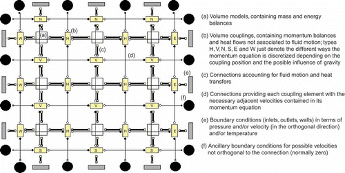
Figure 3 shows that the grid on which the Navier–Stokes equations are discretized can be represented in a modular way, where volume models are connected together with coupling models. Volume models are of a single type, while coupling ones can be of ‘internal’ or ‘boundary’ type. Figure 4 represents the same situation (in a 3 × 3 volume case for readability) as seen in the Modelica graphical editor.

Figure 3. Transition between the standard grid and its modular representation.

Figure 4. Modelica connection scheme for a 3 × 3 room.

As can be seen, the staggered grid corresponds in Modelica to a modular structure composed only by the main model classes volume, coupling and boundary, with a uniform interface.

Volume models contain the mass balance Equation (4)(4), the energy balance Equation (5)(5), the fluid state Equation (30)(30), the specific energy Equation (34)(34) and the specific enthalpy Equation (35)(35). In Figure 4 they are the square boxes denoted by (a).

Coupling models contain the momentum balance terms (12), (18) and (20), the turbulence model (39) and the heat flow Equation (36)(36). In Figure 4 they are the rectangular boxes denoted by (b): the specializations depending on their position (North, South, East, West, Horizontal, Vertical) just affect the way the contained equations are discretized and can be easily managed by having the position as a further model parameter.

Boundary models contain the momentum balance terms (20), (24) and (28) and the heat Equation (37)(37). For merely practical reasons it was decided to split boundary models in two Modelica elements, indicated in Figure 4 by the narrow grey rectangles (e) and the black circles (f). Collapsing both parts of the boundary conditions in a single element is possible but would result in a more complex connection structure.

Connectors are in fact very simple with the adopted choices. Square ones, linked in Figure 4 by the thick connection lines (c), contain the information on the fluid state and that used by the coupling elements to solve the momentum equation, namely relative pressure, absolute temperature, fluid velocity through the face, heat flow rate through the face, specific enthalpy flowing through the face, density of the fluid flowing through the face, velocities associated the other faces of the volume and sizes of the volume. Round connectors, linked in Figure 4 by the thin lines (d), connect coupling/boundary elements providing the velocity of surrounding coupling elements, and the distance between the said elements.

As a result, constructing a compound model (also in the foreseen 3D case) is very easy by means of array structures. Compound models such as those of the following examples are spatially parametrized by just providing their dimensions, and the number of volume divisions (not necessarily evenly spaced) along the coordinate axes. Also, replacing the fluid state equation with a different one is very straightforward, as is modifying the turbulence model.

5. Validation

Some validation tests are now reported with reference to literature results. Simulation time information is also given, to prove the efficiency advantages of the proposed approach over alternative ones. All the presented simulations were obtained on a standard PC, using Dymola [41] as the Modelica translator.

5.1. Poiseuille motion in a duct

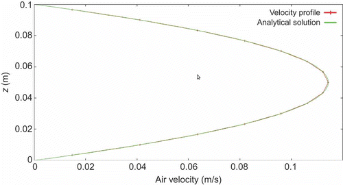
The first test deals with laminar flow, to exclude possible effects of the turbulence model (i.e. μ _T  = 0). The addressed case is fluid motion in a duct, for which under certain assumptions it is possible to find an analytic solution. An example is the so-called Poiseuille motion [42], that is, laminar flow in a circular (horizontal) duct. The Poiseuille equations relate the mean velocity of the fluid and the pressure drop between the duct endpoints, and allow to compute the exact steady velocity profile on the duct section: as shown in Figure 5 and demonstrated by Poiseuille, the said profile is a parabola.

Figure 5. Horizontal duct with laminar flow.

In this test, the presented models are used to obtain the velocity field in a horizontal square duct. By suitably adapting the Poiseuille formula to the square case, it turns out that if the flow is laminar, also the velocity profile on the two planes orthogonal to the duct lateral faces and containing the axis are parabolic. The maximum velocity is on the duct axis and its value is (h ² Δ P)/(8 μL), and the mean fluid velocity equals (h ² Δ P)/(12 μL). A laminar flow simulation obtained with the devised model is shown in Figure 5, and comprises a 2D grid composed of I × K elements in the x and z directions, respectively. Note that the grid does not need to be equally spaced.

Figure 6 shows how the mean velocity provided by the model approaches the analytical solution when increasing the number of volumes along z and x. As expected, while the number of volumes along z plays a crucial role in the approximation of the analytic solution, the number of volumes along x is less relevant. Figure 7 reports the steady-state (parabolic) velocity profile at the duct end section.

Figure 6. Mean x velocity on the duct end section versus (a) K (number of volumes along z) and versus (b) I (number of volumes along x).

Figure 7. Steady-state velocity profile on the duct end section.

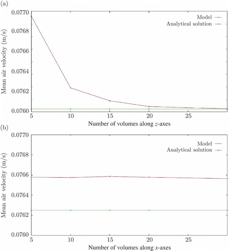
This example proves the model correctness in a case where the analytic solution is known. The simulation efficiency is good: for example, a 300 s simulation of a duct model composed by 5 × 15 volumes takes 0.25 s on a standard PC. Of course the accuracy is not comparable to that of full-fledged CFD codes, nonetheless it is definitely more than sufficient for the targeted applications. It is also worth stressing that with the presented model a dynamic simulation is performed, while with standard CFDs only static solutions are often provided and the computational burden of dynamic ones, when available, is far higher.

5.2. Room with natural convection

The second test refers to a case where turbulence matters. The experimental and simulation results of [43] and [29] are taken here as reference. The experimental set-up in the quoted works is the MINIBAT test cell at CERTHIL, described in [44], that consists of a 24 m³ (3.1 m × 3.1 m × 2.5 m) volume where the temperature is kept constant on five faces. The sixth face is in contact with a climatic caisson, which allows the air temperature to be controlled in the range from –10°C to 40°C with a very good stability (±0.2°C).

The case shown here has two walls with impressed temperature: with reference to the naming of Figure 4, the west one is ‘cold’ and the east one is ‘hot’; north and south temperatures are not impressed. Since the environment is actually 3D, the 2D grid is here complemented by exchanges with the ‘front’ and ‘rear’ walls, with obvious meaning. The said exchanges are described with classical correlations: heat transfer is assumed to be linear in the surface-to-air temperature difference, with a heat transfer coefficient of 4.1, 1.0 and 4.7 W/m K for walls, floor and ceiling, respectively [30].

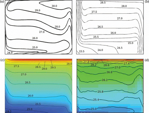
The temperature distribution provided by the presented models is shown in Figure 8(c), that reports also (a) the experimental results of [43], (b) the results of another simulation tool (COMIS, see [29]) with a similar approach to the one presented, and the simulation results provided by the fine-scale 3D CFD tool Code_Saturne [45]. As can be seen, Modelica results are in reasonable agreement not only with those from the similar tool COMIS, but also with those from Code_Saturne, and all the presented tools yield more or less the same level of discrepancy with respect to experimental results. Finally, here too, efficiency is good: on a standard PC, a 3000 s simulation takes approximately 1.5 s only with a 12 × 10 grid (the same resolution used in the quoted COMIS reference). No information is available on the COMIS simulation time, but 1.5 s is indeed a hard-to-beat result, not to mention the modularity advantages of the proposed approach. As for Code_Saturne, for which a cubic mesh of 25³ elements was used, the simulation run that produced the results of Figure 8(c) required about 15 min.

Figure 8. Temperature distribution within the room (°C) with natural convection: experimental data (a) and simulation results of COMIS (b), the presented Modelica models (c) and Code_Saturne (d).

6. Conclusions and future work

An OOM approach has been proposed to somehow emulate CFD-based results in the context of building simulation. By means of an ad hoc equations' formulation and model structuring, high modularity and simulation efficiency can be achieved. Of course, the presented models do not fully replicate CFD results, but allow us to preserve the relevant facts for energy-related simulation studies. In addition, said models can be readily integrated in a multi-physics environment, thereby avoiding the use of co-simulation to the advantage of speed and model maintenance.

Future work will be devoted to extending the proposed framework to the 3D case, which is however quite straightforward, and to the representation of complex geometries. Further validations will also be carried out, and the obtained models will be integrated in a general-purpose building simulation library, taking particular care to ease the model parametrization for a better usability.

References

- Haves , P. , Salsbury , T. , Claridge , C. and Liu , M. 2001 . “ Use of whole building simulation in on-line performance assessment: Modeling and implementation issues ” . In Proceedings of the 7th International IBPSA Conference , 335 – 342 . Rio de Jeneiro Brazil, International Building Performance Simulation Association (IBPSA) .
- E. Mazria and K. Kershner, Meeting the 2030 challenge through building codes, 2008. Available at(1 June 2011) http://www.architecture2030.org/ (http://www.architecture2030.org/)
- Sahlin , P. 2000 . “ The methods of 2020 for building envelope and HVAC systems simulation – Will the present tools survive? ” . In Proceedings of the CIBSE Conference Dublin, , Ireland
- Wetter , M. and Haves , P. 2008 . A modular building controls virtual test bed for the integration of heterogeneous systems, Proceedings of the 3rd National Conference of IBPSA-USA Berkeley, CA
- Wetter , M. 2009 . Modelica-based modeling and simulation to support research and development in building energy and control systems . J. Build. Perform. Simul. , 2 ( 1 ) : 143 – 161 .
- Janak , M. 2000 . Coupling building energy and lighting simulation, Proceedings of the 5th International IBPSA Conference Kyoto, , Japan
- Wetter , M. 2009 . Modelica library for building heating, ventilation and air-conditioning systems, Proceedings of the 7th International Modelica Conference 393 – 402 . Como, , Italy, The Modelica Association, Linköping, Sweden
- Djunaedy , E. , Hensen , J.L.M. and Loomans , M.G.L.C. 2003 . Towards external coupling of building energy and air flow modeling programs . ASHRAE Trans. , 109 ( 2 ) : 771 – 787 .
- Li , N. , Wang , Z. , Liu , W.H. , Peng , X.Y. and Gong , G.H. 2005 . Research on construction and interoperability of complex distributed simulation system . Lect. Notes Comput. Sci. , 3398 : 131 – 140 .
- Follen , G. , Kin , C. , Lopez , I. , Sang , J. and Townsend , S. 2001 . A CORBA-based development environment for wrapping and coupling legacy scientific codes, 10th IEEE International Symposium on High Performance Distributed Computing 22 – 31 . San Francisco, CA, IEEE, New York
- Gu , B. and Asada , H. 2004 . Co-simulation of algebraically coupled dynamic subsystems without disclosure of proprietary subsystem models . ASME J. Dyn. Syst. Meas. Control , 126 ( 1 ) : 1 – 13 .
- Huang , J. , Winkelmann , F. , Buhl , F. , Pedersen , C. , Fisher , D. , Liesen , R. , Taylor , R. , Strand , R. and Lawrie , L. 1999 . Linking the COMIS multi-zone airflow model with the EnergyPlus building energy simulation program, Proceedings of the 5th International IBPSA Conference Kyoto, , Japan
- Taylor , S.J.E. , Bruzzone , A. , Fujimoto , R.M. , Gan , B.P. , Strassburger , S. and Paul , R.J. 2002 . Distributed simulation and industry: Potentials and pitfalls, Proceedings of the 2002 Winter Simulation Conference San Diego, CA
- Allard , F. , Dorer , V.B. and Feustel , H.E. 1990 . Fundamentals of the multizone air flow model COMIS . Tech. Note 29, AIVC, Coventry, UK ,
- Feustel , H.E. 1999 . COMIS – An international multizone air-flow and contaminant transport model . Energy Build. , 30 ( 1 ) : 3 – 18 .
- Haghighat , F. , Li , Y. and Megri , A.C. 2001 . Development and validation of a zonal model – POMA . Build. Environ. , 36 ( 9 ) : 1039 – 1047 .
- Walton , G.N. 1997 . CONTAM’96 Users Manual , Gaithersburg, MD : NISTIR 6055, National Institute of Standards and Technology .
- Drury , B. and Crawley , B. 2000 . EnergyPlus: Energy simulation program . ASHRAE J. , 42 ( 4 ) : 49 – 56 .
- Fluent Inc., Fluent 6.1 Tutorial Guide, Fluent Inc., Lebanon, NH, 2003.
- Fluent Inc., Fluent 6.3 User's Guide, Fluent Inc., Lebanon, NH, 2003.
- Felgner , F. , Agustina , S. , Bohigas , R.C. , Merz , R. and Litz , L. Simulation of thermal building behaviour in modelica . Proceedings of the 2nd International Modelica Conference . Vol. 154 , Citeseer, Oberpfaffenhofen, , Germany
- Wetter , M. Multizone airflow model in Modelica . Proceedings of the 5th International Modelica Conference . Vienna, Austria. Vol. 2 , pp. 431 – 440 .
- Fritzson , P. 2004 . Principles of Object-Oriented Modeling and Simulation with Modelica 2.1 , Hoboken, NJ : Wiley-IEEE Press .
- Wetter , M. and Haugstetter , C. 2006 . “ Modelica versus TRNSYS – A comparison between an equation-based and a procedural modeling language for building energy simulation ” . In Proceedings of the 2nd National Conference of IBPSA-USA Cambridge, MA
- Merz , R. 2002 . Objektorientierte mathematische modellierung thermischen Gebäudeverhaltens (in German) , Ph.D. thesis, Department of Electrical Engineering, University of Kaiserslautern .
- Sodja , A. and Zupančič , B. 2009 . Modelling thermal processes in buildings using an object-oriented approach and Modelica . Simul. Model. Pract. Theory , 17 ( 6 ) : 1143 – 1159 .
- Felgner , F. , Merz , R. and Litz , L. 2006 . Modular modelling of thermal building behaviour using Modelica . Math. Comput. Model. Dyn. Syst. , 12 ( 1 ) : 35 – 49 .
- Mora , L. , Gadgil , A.J. and Wurtz , E. 2003 . Comparing zonal and CFD model predictions of isothermal indoor airflows to experimental data . Indoor Air , 23 ( 2 ) : 77 – 85 .
- Ren , Z. and Stewart , J. 2003 . Simulating air flow and temperature distribution inside buildings using a modified version of COMIS with sub-zonal divisions . Energy Build. , 35 ( 3 ) : 257 – 271 .
- Wurtz , E. , Nataf , J.M. and Winkelmann , F. 1999 . Int. J. Heat Mass Transf . Two- and three-dimensional natural and mixed convection simulation using modular zonal models in buildings , 42 ( 5 ) : 923 – 940 .
- Felgner , F. 2008 . Design of Virtual Airflow Sensors for Thermal Comfort Control , Aachen : Shaker Verlag .
- Mattsson , S.E. , Elmqvist , H. and Otter , M. 1998 . Physical system modeling with Modelica . Control Eng. Pract. , 6 : 501 – 510 .
- Modelica Association Modelica home page. Available at (1 June 2011). http://www.modelica.org/ (http://www.modelica.org/)
- Patankar , S.V. 1980 . “ Numerical Heat Transfer and Fluid Flow ” . In Taylor & Francis London
- Versteeg , H.K. and Malalasekera , W. 2007 . An Introduction to Computational Fluid Dynamics: The Finite Volume Method , Upper Saddle River, NJ : Pearson Prentice Hall .
- Chow , P. , Cross , M. and Pericleous , K. 1996 . A natural extension of the conventional finite volume method into polygonal unstructured meshes for CFD application . App. Math. Model. , 20 ( 2 ) : 170 – 183 .
- Lien , F.S. 2000 . A pressure-based unstructured grid method for all-speed flows . Int. J. Numer. Meth. Fl. , 33 ( 3 ) : 355 – 374 .
- Tasri , A. 2010 . Simple improvement of momentum interpolation equation for Navier-Stoke equation solver on unstructured grid . J. Math. Stat. , 6 ( 3 ) : 265 – 270 .
- Wilcox , D.C. 2006 . Turbulence Modeling for CFD , 3rd , La Canada, CA : DCW Industries .
- Chen , Q. and Xu , W. 1998 . A zero equation turbulence model for indoor airflow simulation . Energy Build. , 28 ( 2 ) : 137 – 144 .
- Dassult Systèmes, Dymola 7.4 www.3ds.com/products/catia/portfolio/dymola (http://www.3ds.com/products/catia/portfolio/dymola)
- Bennett , C.O. and Myers , J.E . 1962 . Momentum, Heat, and Mass Transfer , New York : McGraw-Hill .
- Inard , C. , Bouia , H. and Dalicieux , P. 1996 . Prediction of air temperature distribution in buildings with a zonal model . Energy Build. , 24 ( 2 ) : 125 – 132 .
- Allard , F. , Brau , J. , Inard , C. and Pallier , J.M. 1987 . Thermal experiments of full-scale dwellings cells in artificial conditions . Energy Build. , 10 ( 1 ) : 49 – 58 .
- Archambeau , F. , Méchitoua , N. and Sakiz , M. 2004 . Code Saturne: A finite volume code for turbulent flows . Int. J. Finite , Vol. 1 ( 1 ) : 1 – 62 .