Modelling and long-term simulation of a heat recovery steam generator

Abstract

Developing accurate non-linear dynamical models for heat recovery steam generator (HRSG) units is presented in this article. The common non-linear autoregressive with exogenous input (NARX) system topology was employed to develop the neuro-fuzzy models based on the experimental data taken during field experiments. In this structure, the non-linear behaviours of the HRSG unit can be characterized through interpolation of local linear models associated with different operating regions via fuzzy inference mechanism. The operating regimes were recognized by applying a genetic algorithm-based fuzzy clustering technique to the prepared data sets. The structures of the fuzzy models are defined with respect to the obtained optimal cluster centres and the corresponding membership functions. The parameters of fuzzy rules were adjusted by recursive least-squares estimation method to fit the model responses to real data. The performances of developed models were evaluated by performing a comparison between the model responses and the responses of the real plant. In addition, the stability of the developed models was assessed by perturbing the model inputs from the nominal values. This guarantees the long-term simulation capabilities of the developed models. A comparison between the responses of the corresponding models and the models obtained from some recent modelling approaches was performed to show the advantages of the developed models. The results show the accuracy and reliability of the developed models at transient and steady-state conditions.

Keywords:

• heat recovery steam generator
• non-linear behaviour
• experimental data
• fuzzy system
• clustering method
• genetic algorithm

1. Introduction

Long-term dynamics simulation has been known as a main key for performance evaluation, fault detection and process optimization of thermal power plants [1–4]. For many years, researchers and engineers have been interested in developing accurate mathematical models, including entire subsections, control systems and protective functions. Inherent non-linear behaviour, load-dependent dynamics, exposure to large disturbances and many safety limitations can cause difficulty in developing an appropriate model, which could describe the effects of variations of inputs, outputs and internal parameters on the plant performances [5–7].

In the presence of adequate information from real plant performances, utilizing black-box structure would be an appropriate method to develop a mathematical model that could virtually characterize relationships between input–output variables [8,9].

Applying system identification techniques to the measured data taken during experiments is a common way to develop data-driven models. Linear models have been employed for analysing the dynamic behaviours of thermal power plants for decades. Choosing appropriate input–output data sets that govern the system dynamics is the main key for developing accurate linear models [10,11]. However, the effects of some physical characteristics such as specific density or heat capacities, which are dependent on operating conditions, are often ignored in linear models [11]. Within a specific working range, linear models are effective tools for prediction purposes or purposes of controller design. Different types of linear models with autoregressive with exogenous input (ARX), autoregressive moving average exogenous input (ARMAX), output error (OE) and Box–Jenkins (BJ) structures have been employed in a wide range of applications for dynamic system analysis [11,12], simulation [13], controller designing [14,15], performance monitoring [16] and fault diagnosis [17,18]. Linear models can also be employed for optimization purposes. However, due to the non-linear behaviours of thermal plants, a set of different linear models may be required to cover all operating ranges. In this case, employing a combination of local linear models in order to build a non-linear model is recognized as a good solution [19,20]. This technique has been commonly employed in model predictive controllers that provide more reliable operation with less computational efforts in real applications [21,22].

In recent years, many modelling approaches have been proposed that are able to interpolate the linear models corresponding to different operating conditions to describe the dynamics of non-linear systems. A major group of these works has been associated with non-linear system modelling based on artificial intelligence that comprises different areas such as artificial neural networks (NNs), fuzzy logic (FL), evolutionary computing and hybrid systems [23,24]. Adaptive neuro-fuzzy inference system (ANFIS) is one of the most common structures used for non-linear system modelling, in which the fuzzy if–then rules are represented in a network structure [25]. This system can be enforced in combination with other soft computing approaches to deal with complicated and uncertain systems. Many applications of neuro-fuzzy modelling have been reported in different industrial areas, including power plants. This can be addressed in the works done by Fantoni et al. [26], Vieira et al. [27], Abdelazim and Malik [28], Kothamasu and Huang [29], Ghaffari et al. [30], Kishor [31], Esen and Inalli [32], da Costa et al. [33] and Peña et al. [34].

Despite good performance of conventional ANFIS structure, it suffered from high number of tunable parameters that might lead to model overfitting problems (for very small data sets) or cause the process of model training to become time consuming or practically impossible (for very large data sets). Furthermore, the structure identification of fuzzy systems is generally a great problem in developing accurate test data-based models with reasonable degree of complexity. To deal with this problem, different partitioning approaches were proposed to define the structure of fuzzy systems and in order to reduce the number of fuzzy rules with minimum loss of accuracy [35–37]. The fuzzy c-means (FCM) clustering method was introduced by Dunn in 1973 to organize a data set by its partitioning into smaller subsets to reveal the structure of fuzzy system [38]. This technique allows a non-linear system to be approximated through interpolation of local linear models associated with different operating regions via fuzzy inference mechanism. This approach could be very useful for the modelling of industrial processes [39,40].

This article presents an application of genetic algorithm (GA)-based fuzzy clustering approach for developing accurate non-linear models for a heat recovery steam generator (HRSG). By decomposing the entire unit into smaller subsystems, the governing variables of each subsystem are recognized and the required data are prepared through field experiments. Each subsystem is considered as a multi-input single-output (MISO) neuro-fuzzy model. FCM clustering is employed to recognize the operating regions and to identify the structure of the models. An optimization approach based on GA is employed to solve non-linear optimization problem by minimizing c-means objective function in order to find best cluster centres and the corresponding membership functions (MFs). The parameters of consequents are captured using least-squares techniques based on input/output data. The accuracy of developed models is validated by performing a comparison between the responses of developed models and actual data in different operating conditions. Furthermore, a comparison between the response of the developed models and the models obtained from other recent modelling approaches was preformed to evaluate the feasibility and performance of the proposed modelling approach. In addition, the performance of the closed loop system is evaluated as the unit load is ramped up from 44.2% of nominal load to full-load conditions.

In Section 2, the architecture of neuro-fuzzy system is presented. The procedure of identifying the structure of fuzzy models and data partitioning are presented in this section. In Section 3, a brief description of the plant that consists of a general view of the power plant and its subsystems is presented. The inputs and outputs in the subsystems are also specified in this section. Developing the HRSG subsystem models based on the experimental data, simulation experiments and model validation is presented in Section 4. The closed responses and long-term simulation are presented in Section 5 to evaluate the performance of the overall plant. The last section reports the conclusion and some suggestions for future work.

2. Neuro-fuzzy model

Many different types of FL models have been employed to approximate and capture the dynamics of uncertain and complex systems. In general, a dynamic fuzzy model can be developed by using the common non-linear autoregressive with exogenous input (NARX) input–output model topology as follows:

(1)

These models are constructed as a discrete-time non-linear model mapping on some prior measured inputs and outputs of the system as follows:

(2)

The non-linear mapping function f(·) can be enforced by NN computational machines, which is known as the ANFIS. ANFIS, which was originally developed by Jang in the early 1990s benefited from fuzzy reasoning ability and robust and rapid adaptation capability of NNs. The Takagi, Sugeno and Kang (TSK) type of fuzzy models is a well-known architecture extensively used as the core of ANFIS. A general form of fuzzy rules in TSK fuzzy models is a linear combination of the input variables plus a constant term, which is known as the first-order TSK [25]. By partitioning input space into several subspaces, each rule would represent a local linear model at the corresponding regime, which prepares a soft transition between different operating conditions [36,37]. For a first-order TSK fuzzy model, a typical rule set can be expressed in the form of if–then rules:

(3)

In Equation (3(3)), A_i,j is the MF associated with input variable x_j , where j and i are the number indices for the inputs and MFs, respectively.

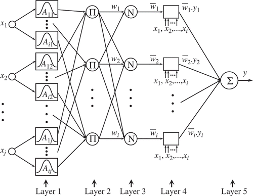
In Figure 1, the architecture of ANFIS for the TSK fuzzy model is presented. In this structure, the firing degrees of the fuzzy rules are calculated through the five layers of the model [41]:

Figure 1. The ANFIS architecture of Sugeno model.

In layer 1, the MF A_i,j which is considered to be Gaussian is specified by the centre v and the spread σ, as presented in the following equation:

(4)

In layer 2, the fulfilment degrees of rules are calculated by multiplying the output values of all MFs as follows:

(5)

where n is the number of fuzzy model inputs that equals the sum of the input and output lags, (n_u + n_y ), presented in Equation (2)(2). In layer 3, the firing strength of each fuzzy rule is defined by calculating the relative degree of fulfilment as follows:

(6)

where c is the number of MFs for the inputs. Here, the identical numbers of MFs are considered for all the inputs. In layer 4, the normalized firing strengths from layer 3 are multiplied by the consequents:

(7)

In layer 5, the output of fuzzy system is calculated by summation of all weighted consequents of the fuzzy rules:

(8)

As the neuro-fuzzy system is formulated, the model parameters can be tuned with respect to training data using a learning algorithm. Therefore, the input–output patterns can be defined as

(9)

The parameters of the matrix Θ and MFs should be adjusted based on the experimental data. It is noted that the number of fuzzy rules is equal to the number of MFs powered by the number of inputs. In order to reduce the number of fuzzy rules and consequently the number of parameters, a fuzzy clustering algorithm was employed to define the structure of fuzzy systems.

2.1. Data clustering and fuzzy structure

In this section, the operating regions are verified by applying clustering technique on recorded data set. For this aim, a GA-based fuzzy clustering approach is employed to define the fuzzy model structure. FCM clustering is one of the most common techniques used for data organizing based on the optimization of the basic c-means objective function [42]. This algorithm is for partitioning the input data space into c predefined subsets through optimizing an objective function, which indicates the desirability of each c-partition. The data partitioning into clusters depends on the similarity/dissimilarity of each cluster member, which is generally defined by the distance of data points from cluster centres [43,44].

An unlabelled data set Z = {z ₁, …, z_n } ⊂ R^s can be partitioned into the given c subsets represented as fuzzy sets F = {F ₁, …, F_c } with cluster centroids vector V = {v ₁, …, v_c } ⊂ R^s . By defining the distance function D(vⁱ ,z^j ) as the Euclidean norm between vⁱ and z^j , we have

(10)

The following objective function has to be minimized in order to obtain the best possible solution:

(11)

where U = [u_ij ] _c×n and u_ij is the membership degree of the jth data point in the ith cluster. The weighting exponent m (1 ≤ m < ∞) determines the fuzziness degree of each datum membership. The membership matrix is calculated by the following equation:

(12)

In this work, an optimization approach-based GA is employed to solve a non-linear optimization problem by minimizing the objective function J_m . GAs are stochastic optimization techniques that are able to find best possible results in the entire solution space. The main advantages of GAs are their ability to discover global optimum, wider solution space, resistant to becoming trapped in local optima and the robustness in objective function evaluation. This approach is particularly useful for non-linear systems working at different operating conditions. The optimization is performed to find the best possible cluster centres, {v_i }, by considering the following constraints on the membership values, which would lead to the optimal partition:

(13)

In order to handle possible solutions, GA creates an initial random population and evaluates fitness function for each population. The next searching points are determined by minimizing the fitness values of multiple current searching points. New populations are iteratively generated by either copying the selected individuals or applying GA operators (mutation, crossover, reproduction, selection, etc.) in order to attain smaller fitness values [45,46].

The GA-based fuzzy clustering was implemented in m.file code named as ‘anfsgaclstrng.m’, in which a simple Picard iteration algorithm was replaced by GA. The MATLAB function ‘ga’ is employed as the optimization agent in the core of the developed codes (available on http://wmail.kntu.ac.ir/chaibakhsh/project.html). The centres of clusters are captured by minimizing the fitness function (11) and with respect to constraints (13). In order to increase the performance of optimization, the data set was normalized to lie in the range of [–1,1]. Lower and upper bounds on the variables and initial populations are also defined to reduce computational efforts. The default optimization parameters for GA are presented in Table 1. In order to run the program, a predefined number of clusters c are required, which can be chosen manually or by using subtractive clustering algorithm. The procedure of implemented algorithm is presented in Table 2.

Table 1. The optimization parameters for GA

Optimization parameters	Type/value
Population size	100
Crossover	Single point
Crossover rate	0.7
Mutation	Gaussian/scale = 1/shrink = 0.7
Reproduction	Elite count:2
Selecting	Stochastic uniform
Migration	Forward/0.1
Generations	200

Table 2. Procedure of fuzzy clustering by GA

1. Normalizing data set {zi } by dividing on max(abs({zi }))

2. Defining the number of variables

−  number of parameters = (data size) × c

3. Determining lower and upper bounds on variables.

−  lb = min({zi })/max(abs({zi }))

−  ub = max({zi })/max(abs({zi }))

4. Determining lower and upper bounds of initial population

−  rang = min({zi })/max(abs({zi })) + (1 – min({zi })/max(abs({zi })))/c × i ∀ i=1… c

−  lrang = rang –0.1

−  urang = rang +0.1

5. Performing GA optimization to determine {vi } such that the fitness function Jm is minimized

−  Calculating Dij from Equation (10)(10).

−  Calculating uij from Equation (12)(12).

−  Calculating Jm from Equation (11)(11).

6. Extracting the parameters of MFs from results and creating FIS.

7. Adjusting the parameters of fuzzy rules.

The performance of the proposed algorithm is evaluated on two different data sets. In Figure 2(a), a data set with 800 samples with seven clusters and some noisy points is presented. In addition, a very noisy data set with 300 samples is prepared, which is shown in Figure 2(b). As it is shown, the proposed algorithm is able to find cluster centres perfectly in noisy data spaces.

Figure 2. A data set with seven cluster centres (a) and a noisy data set with five cluster centres (b).

2.2. Tuning the parameters of consequents

The developed code is able to find cluster centre for Sugeno and Mamdani systems. For Sugeno-type systems, by defining the fuzzy MFs and the corresponding fuzzy rules, the parameters of consequents can also be tuned. For this purpose, at the fourth layer of the neuro-fuzzy system, least-squares estimation (LSE) is used to find the consequent parameters as follows:

(14)

For achieving better performances, generated fuzzy interference system (FIS) is used as the initial FIS for the conventional ANFIS training, where a combination of LSE and backpropagation (BP) methods is employed to adjust the parameters of MFs and consequents. However, no considerable changes would be observed in the MF parameters. As a result, in this work the ANFIS training mechanism was employed instead of LSE.

3. HRSG description and subsystems

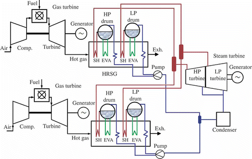
In modern power plants, in order to increase the overall performance of thermal units, the exhaust heat from gas turbines is recovered from HRSG boilers. In this study, one of the HRSG boilers of two combined cycle units of the Neka power plant (at the north of Iran) was considered for investigation. Each unit consists of two V94.2 gas turbines, one horizontal-type HRSG plant and high-pressure (HP) and low-pressure (LP) steam turbine units. A schematic diagram of the power plant is shown in Figure 3. The rated powers of the gas and steam units are 2 × 137.5 MW and 160 MW, respectively.

Figure 3. The combined cycle power plant configuration.

In combined cycle power plants, the exhaust gas from gas turbines is recovered from HRSG. The hot exhaust gas from turbine and three auxiliary burners provides the required heat for this boiler. The output temperature of the gas turbine is about 530°C, which burns natural gas as the main fuel. The HRSG boiler consists of different parts such as deaerator, economizer, LP drum, HP drum, evaporators, superheaters and desuperheaters.

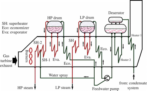
In Figure 4, the details and configuration of HRSG are presented. As it is shown, the feedwater from condensation system heads to the deaerator and is passed through first preheating section. In the storage tank, its temperature will increase to 80°C and then is sent to the feedwater pump to increase its pressure. A part of the feedwater is fed to the LP drum in order to be converted to steam. The output pressure and temperature at the header of LP drum are about 0.85 MPa and 235°C, respectively, where the nominal steam flow rate is 9 kg/s. The evaporated steam goes to the LP superheating section, and then enters to the LP sections of the steam turbine. The generated steam in LP section has no effect on the turbine power; however, its role is very important for controlling moisture in steam turbine stages.

Figure 4. The configuration of HRSG with auxiliary burners.

The other portion of the feedwater is pumped to the HP economizer to raise the temperature of the feedwater, which increases the boiler efficiency. The hot feedwater goes to the HP drum to be converted to steam. The steam temperature at the drum header is 300°C, where its pressure is about 9.2 MPa. The evaporated steam goes to the primary and final HP superheaters.

The temperature at outlet header of the final superheater will reach 520°C, where its pressure is about 9 MPa and the nominal steam flow rate is 67 kg/s. The superheated steam is flashed to the HP stages of steam turbine.

The expanded steam in HP and LP sections is discharged into the main condenser. The condensate water mass flow rate is 75 kg/s and its temperature is about 52°C. This water, after some chemical treatments, would go to the deaerator and the cycle would repeat.

3.1. Input–output description

The major concern in developing a fuzzy model is with the recognition of proper variables that govern the characteristics of a complicated process. In order to ease the process of system identification, it is recommended that the process be decomposed into smaller components. Then, the dynamic behaviour of each subsystem is characterized in terms of its own input and output variables. The dynamics of a drum boiler were perfectly described by Åström and Bell [47], which was remarkably helpful in this regard.

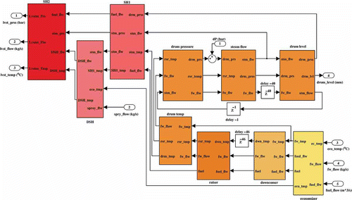
The subsections of the boiler are shown in Figure 4. As it was mentioned before, two main sources are available to provide the required heat for this boiler: the heat of the gas turbines exhaust and duct burners. In this case, the overall heat rate for the HRSG boiler is calculated by summing the fuel burned in each of the gas turbines and the fuel burned in the burners. The heat released by fuel combustion is transferred to the working fluid at different parts of the boiler. As a result, the fuel flow rate is considered as the main input for the boiler subsections. The feedwater flows through the economizer which is the first section. As shown in Figure 4, two economizers are located in the boiler. The heat absorbed by each section is a portion of the total heat released. The other effective variables of the economizer output temperature are known as feedwater mass flow and input water temperature. The input/output vectors of the economizer model are summarized as follows:

(15)

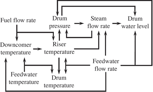
In drum boiler, the supplied heat to riser tubes causes water to turn into steam, where the drum water flows into the downcomer and forces the saturated steam to leave the riser due to gravity, which is causing a circulation in the riser–drum–downcomer loop. The dynamics of these processes are very complicated that many variables may be considered to achieve a reliable prediction. In order to describe the non-linear behaviour of drum boiler, the effects of the state variables, inputs and outputs have to be identified. The entire plant is decomposed into smaller subsystems. In Figure 5, the relationships between the model variables are illustrated. The distributions of steam and water in riser and downcomer are the functions of the supplied heat to the wall. In a natural circulation drum-type boiler, the wall temperatures of downcomer and riser tubes are the only measurable variables.

Figure 5. The effects of inputs, outputs and state variables in a drum steam generator.

The flowing input/output variables are considered to describe the dynamics of downcomer section:

(16)

where the input/output variables for the riser model are as follows:

(17)

The dynamics of the drum pressure are dominated by the changes in energy stored in masses of water and metal [47]. The volume of water entering the drum and the volume of steam leaving the drum have most significant effects on the drum pressure. The riser wall temperature is a good representation of the heat absorbed by the working fluid. Consequently, the input/output variables for the drum pressure model are chosen as

(18)

The steam flow rate is a function of the drum pressure, feedwater flow rate and the steam from riser that can be related to the riser temperature. As a result, the input/output for steam flow rate can be considered as follows:

(19)

The saturated steam from the drum goes towards superheating sections, as the fresh feedwater is supplied to the boiler in order to keep the drum level constant. During a rapid change in feedwater/steam flow or heating rate, severe variations in water level may occur. This phenomenon is known as the shrink-and-swell effect which is a result of the water density changes due to pressure swings in the drum. However, the firing rate has an effect on drum level, but the pressure drop in drum is known as the major cause of swell and shrink [48]. As a result, three elements of steam flow rate, feedwater flow rate and drum pressure can be used effectively in order to predict the water level in the drum:

(20)

The temperature of the steam that leaves the drum is affected by feedwater temperature, saturated steam temperature and feedwater flow rate:

(21)

The hot steam from drum outlet header goes to superheating sections to increase its thermal energy. Fuel flow rate, steam temperature and mass flow rate to the superheater sections are considered as the main variables to predict the superheated output temperature. No pressure loss or any drop in steam flow rate is considered in this section. The input/output vectors of the superheater model are considered as follows:

(22)

The output temperature of the HP superheaters has to be regulated around 520°C. For this aim, between two parts of the HP superheaters, the desuperheating sections consisting of spray water attemperators are considered. By neglecting the pressure loss in the attemperator, the output temperature of the desuperheater can be estimated with respect to the inlet temperature and flow rate of the superheated steam and the temperature and flow rate of the water spray. Therefore, the input/output vector for the desuperheater sections would be as follows [30]:

(23)

and

(24)

The hot steam goes to the final stage of superheating to increase its thermal energy, where its temperature reaches 520°C:

(25)

The delayed output of each model is also considered as the input of the models. By defining the input–output variables for each subsection, it would be possible to develop the models based on experimental data.

4. Experiments, model development and validation

In this section, the experimental data taken from the real plant are employed to develop the non-linear model of the HRSG's subsections by means of the proposed algorithm in Section 2. For all subsections of the boiler, the fuzzy models were considered as a MISO system with four inputs and one output, except the desuperheater section that has five inputs. The required input–output information for modelling process was taken by performing some field experiments. The recorded data comprise the plant performances at transient and steady-state conditions, noise-free conditions and over a wide operating range as the load of steam units is ramped up from half-load to full-load conditions. A proper data set was recorded using a sampling interval of 1 second for a duration of 9600 seconds. The entire experimental data were divided into two separate data sets, including the training set employed for system identification and the validation set used for model validation. A sensitivity analysis has been performed to evaluate the effects of sample size on the accuracy of dynamic fuzzy models. The results show that by increasing the size of sampling time, the accuracy of fuzzy models would considerably decrease. Both data sets are prepared for a duration of 4800 seconds with a sampling time of 1 second.

The procedure for system identification involves two stages. In the first step, by applying the GA-based fuzzy clustering to the training data, the optimal parameters of the input MFs are captured. The clustering method splits the entire operating range into many smaller regimes, in which the number of fuzzy rules equals the number of cluster centres. The number of cluster centres is chosen manually through different runs to achieve best possible responses. Generally, for thermal analysis of power plants, the entire range of operation is divided into smaller suboperating regions (e.g. 35%, 50%, 75% and 100% of nominal load). Here, for all subsections of the boiler except its drum, the number of cluster centres is chosen to be 4 to divide the operating range into four subregions. For the drum level model, six cluster centres were chosen to deal with the complicated dynamics of this section. By defining the structure of the consequent, the parameters of fuzzy rules can be adjusted in the second step using LSE technique.

4.1. Experiments and simulation results

Simulation experiments were performed in MATLAB® (The MathWorks, Inc., Natick, MA, USA) Simulink environment. The prediction accuracy of the developed models is evaluated by performing a comparison between the responses of the models and the actual plant responses. For this propose, the error functions are calculated for the developed models, where the error is defined as the difference between the predicted values by the models and the experimental data. Here, the upper bound error (Max(|e|)), lower bound error (Min(|e|)), mean absolute error (MAE) and the coefficient of determination (R² ) are calculated over the operating range at transient and steady-state conditions, which are calculated by the following equations:

(26)

(27)

(28)

where is the average of y over the n samples, and and are the ith target and the model output, respectively. The acceptable values of MAE and R ² values would specify the accurate behaviour of the system. The error functions are calculated for the models with respect to the training data, which are presented in Table 3. The results obtained indicate the outstanding performances of the developed models. However, large deviations in the predicted values by riser temperature and drum level models can be observed, where the maximum error values are 3.72 and 2.76 for the riser temperature and drum level models, respectively.

Table 3. Error functions for the developed models with respect to training data

Subsection	Max(|e|)	Min(|e|)	Mean	MAE	R ^2
Economizer	0.2789	8.5e-6	−0.0035	0.0443	0.9994
Downcomer temperature	0.3308	6.9e-6	0.0122	0.0831	0.9996
Riser temperature	3.7189	2.1e-5	−0.2565	0.7632	0.9950
Drum pressure	0.2836	3.3e-6	0.0111	0.0494	0.9999
Steam flow	0.5576	2.1e-5	0.0045	0.0815	0.9997
Drum level	2.7632	0.0014	0.1505	0.5774	0.9751
Drum temperature	0.5192	1.9e-5	0.0039	0.1021	0.9993
Superheater #1	0.8031	1.3e-5	−0.0272	0.1910	0.9995
Desuperheater	0.2527	8.5e-6	0.0057	0.0798	0.9999
Superheater #2	0.4393	2.6e-6	0.0054	0.0826	0.9996

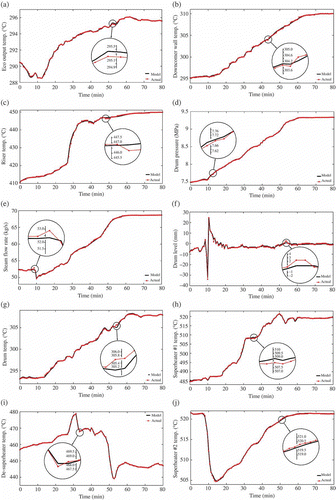
Furthermore, the performances of the developed models are evaluated with respect to the validation data. In Figure 6, the responses of the models and the actual plant are illustrated. The corresponding error functions are calculated and presented in Table 4.

Figure 6. The responses of HRSG subsection models.

Table 4. Error functions for the developed models with respect to validation data

Subsection	Max(|e|)	Min(|e|)	Mean	MAE	R ^2
Economizer	0.2694	2.9e-4	−0.0053	0.0452	0.9994
Downcomer temperature	0.2648	0.0026	0.0045	0.0865	0.9996
Riser temperature	0.9084	0.0026	−0.0505	0.2116	0.9996
Drum pressure	0.2369	1.9e-4	0.0101	0.0511	0.9999
Steam flow	0.5390	4.2e-4	0.0029	0.0739	0.9997
Drum level	2.3121	0.0228	0.1598	0.5502	0.9751
Drum temperature	0.5613	0.0024	0.0014	0.1021	0.9993
Superheater #1	0.8299	0.0014	−0.0185	0.1863	0.9997
Desuperheater	0.2451	0.0014	0.0058	0.0755	0.9999
Superheater #2	0.3847	1.9e-4	0.0103	0.0840	0.9996

In Figure 6(a), the responses of the developed model for the economizer are presented. As it is shown, the feedwater temperature is changing in the range of 288–296°C, where the model is able to follow very well as the maximum error is less than 0.3. The responses of downcomer and riser are shown in Figure 6(b) and (c), respectively. Simulation experiments show that considering a time delay of about 46 seconds in the downcomer temperature input is required to match the predicted values with actual data, which is confirmed by the obtained results presented in Table 4. In Figure 6(d) and (e), the drum pressure responses and steam flow rate are presented, respectively. The effects of the steam flow and the drum pressure are well considered on each other.

Any changes in steam demand may cause a rapid variation in the drum pressure, which would lead to a severe rise or drop in the drum level. The swell and shrink effects would cause a non-minimum phase behaviour in the boiler dynamics, which is much more observable at lower loads. A time delay of about 40 seconds is considered for the feedwater flow input to match the responses of the model and the actual plant. In Figure 6(f), the drum level oscillations are shown at different operating conditions.

The obtained results show that the drum level model was able to predict the swell–shrink effects perfectly; however, the maximum error was not reduced due to unknown source of disturbances.

In Figure 6(g), the responses of the temperature model for the saturated steam leaving the drum section are shown. The responses of primary and final superheaters are shown in Figure 6(h) and (j), respectively. The desuperheating section is considered between these two sections so that the output temperature of the final superheater does not exceed 525°C. By increasing the boiler load and the steam flow rate, the output steam temperature would drop; consequently, the controller would cut off the spray flow to attemperators and the output temperature of the desuperheater would increase. The responses of the developed model for the desuperheater section are presented in Figure 6(i), which indicates this fact very well. The superheated steam would lose about 8°C as it enters the HP turbine. In addition, the stream pressure would drop about 0.3 MPa by passing through each part of the superheating system.

4.2. Test and comparisons

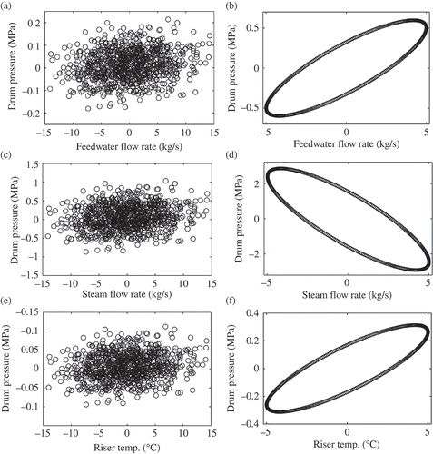
The sensitivity of the developed models can be examined by applying planned perturbations to the input variables and observing their effects on the output variables. Here, the developed models were tested by two different input excitations, where some zero-mean random noise and sinusoidal inputs were applied to the models. The sensitivity analysis was carried out for the drum pressure model as an example. The responses of the drum pressure model are shown in Figure 7. The distributions of the drum pressure variations via the input variable changes are presented in Figure 7(a), (c) and (d), respectively. The model was excited by zero-mean random noise with a power spectral density of 2 and a sampling time of 0.1 second around the nominal operating point. The results show that the steam flow rate is the main dominant parameter of the drum pressure dynamics and by increasing the steam flow rate, the drum pressure would drop. This completely agrees with the nature of drum boilers. In Figure 7(b), (d) and (f), the phase plane diagrams were also plotted for the drum pressure model as the variables were excited by the pure sinusoidal waves (with a magnitude of 5 and a frequency of 0.01 rad/second). Obtained results indicate the stability of the developed models even if large perturbations are applied to the system. A model with these capabilities would be an appropriate option for long-term simulation purposes.

Figure 7. Sensitivity analysis of the developed model for drum pressure.

The performances of the developed models are also evaluated by performing a comparison between the responses of these models and the models obtained from some recent modelling approaches. Three different types of dynamic models are developed for this purpose [49]:

1.	Dynamic fuzzy model. The conventional ANFIS was employed to develop dynamic fuzzy models based on grid partitioning algorithm. The same number of Gaussian MFs is considered for the HRSG subsection models. The parameters of consequents and MFs are adjusted by LSE and BP techniques. The training process was carried out by employing MATLAB FL toolbox (Ver. 2.2.13).
2.	Elman NN. This structure is a common recurrent structure of NN, which was used in many applications. In this structure, the hidden layer output is feedbacked to the network input, which represents a dynamic mapping between the outputs and inputs of the network. The parameters of model were adjusted by BP-based algorithm (standard Levenberg–Marquardt algorithm). The process of model training is performed by using MATLAB NN toolbox (Ver. 7.0.1).
3.	Linear OE model. The OE models are one of the most widely used structures, which are often more realistic models of reality. In this model, the noise is assumed to disturb additively the process output. The LSE method was used to estimate the parameters of the model. Here, the MATLAB System Identification toolbox (Ver. 7.4.2) was employed to develop the polynomial OE models.

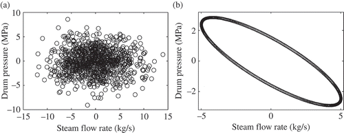
In Table 5, the estimated error functions for the drum pressure, drum level and drum temperature models were presented. The results show that the models with recurrent Elman NN structure have the best performances in comparison with other approaches. The main concern is that such models are very sensitive to input noises. In addition, due to the presence of internal feedbacks in the model structure, any prediction errors would simply deteriorate the performances of the models. The responses of the developed Elman NN model for the drum pressure are presented in Figure 8. As shown in Figure 8(a), the developed model is very sensitive to the rapid changes of input variables. This made the models unreliable for long-term simulations.

Table 5. Error functions for the developed models

	Model type	Drum pressure	Drum level	Drum temperature
Max(|e|)	Elman NN	0.1642	1.1576	0.9416
	ANFIS	0.3766	2.3074	2.6755
	OE model	3.8602	11.5479	5.8709
Min(|e|)	Elman NN	0.0002	0.0031	2.9e-4
	ANFIS	0.0004	1.4e-4	1.9e-4
	OE model	0.0242	0.0047	0.1156
Mean	Elman NN	0.0041	−0.0132	0.1692
	ANFIS	−0.0118	−0.0130	−0.0216
	OE model	−0.0260	−0.0080	−0.6089
MAE	Elman NN	0.0367	0.2677	0.2441
	ANFIS	0.0506	0.2859	0.0836
	OE model	0.8195	1.0111	1.3440
R ^2	Elman NN	0.9999	0.9868	0.9982
	ANFIS	0.9998	0.9693	0.9983
	OE model	0.9729	0.7942	0.9428

Figure 8. Sensitivity analysis of the Elman NN model for drum pressure.

The developed models for boiler subsections are assembled in Simulink® environment, as shown in Figure 9. In order to complete the simulator, some other simple models were added to the plant model. A model for the control valve is required to adjust the inlet pressure of the turbine. The pressure changes at the output header are backpropagated to upper-hand parts particularly the drum section. This is applied through the input port numbered (1) in Figure 9. A pair of boiler supplies the required steam for one turbine.

Figure 9. The HRSG model in MATLAB® Simulink environment.

A simple model for steam turbine was also developed, where the flow rate, pressure and temperature of steam at collector header were considered as the model inputs. For the purposes of system analysis and optimization, it is required that the steam conditions be estimated at the boiler stages. In this regard, a number of simple functions for approximating the thermodynamic properties of water/steam have been developed, which would be able to calculate specific entropy, enthalpy and density with respect to the predicted values of pressures and temperatures [50].

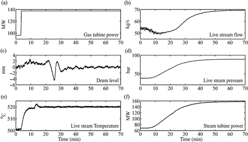
Finally, the performance of the overall plant is evaluated as all control loops are closed. The control systems should be provided to stabilize the overall plant and keep the process variables in tolerable variation ranges. The configuration of employed control systems is presented in Appendix 1. The responses of closed loop system as the loads of gas turbine units are ramped up from 97.5 to 137.6 MW. It is noted that the fuel flow rate is considered as the main input of the HRSG unit model, which can be estimated easily based on the power characteristics of gas turbine units (Appendix 2).

In this case, the loads of HRSG units are ramped up from 44.2% of nominal load to full-load conditions (Figure 10(a)). The obtained results show that the entire subsystems and control systems are working perfectly during load changes.

Figure 10. The closed loop responses of the overall plant.

The flow rate of live steam is presented in Figure 10(b), where more oscillations can be observed at lower loads. In Figure 10(c), the drum level responses are presented. As it is shown, the feedwater controller maintains drum level close to zero set point with respect to the transient signals of steam flow rate, where only small fluctuations can be observed in drum level during load changes. The steam pressure entering the turbine is shown in Figure 10(d), where it has smooth and stable responses with loading gradients of 2%/minute. The output steam temperature is presented in Figure 10(e). The temperature controller is able to keep the temperature constant around 520°C.

It is noted that no desuperheating is required at low-load conditions. In Figure 10(f), the responses of steam turbine are presented in Figure 10(f), where the generated power is ramped up from 70 to 160 MW with changing gradients of 2%/minute. It is noted that the steam turbine loading gradients can be increased up to 10%/minute if sufficient steam pressure is supplied.

5. Conclusion

The purpose of this work was to simulate dynamically a HRSG using FL models. The experimental data taken during field studies were employed to develop neuro-fuzzy models for the unit subsections. A GA-based FCM clustering technique was used to define the structure of fuzzy models and to obtain the parameters of MFs. The parameters of fuzzy rules were tuned using LSE to fit the model responses to experimental data. The responses of the developed models were compared with real data in order to assess their accuracy. The obtained results show a high level of accuracy over a large operating range.

In addition, the performance of the overall unit was evaluated as the load of the units was ramped up from low to full-load conditions. The smooth, precise and stable responses of the plant model during load variations prove the capability of the developed models for long-term simulation. Furthermore, the ability to monitor the HRSG operating parameters such as flow, pressure and temperature at different subsections makes it possible to investigate the effects of any changes on the overall plant performance. This would be of great advantage for optimizing and modifying the operation of power plants.

An increase in power generation efficiency can be obtained through designing a more sophisticated control system. The effects of alternative control systems can easily be evaluated using the developed simulation models. Besides, the developed models can be used directly as the core of model-based predictive control system, advanced fault diagnostic system and fault tolerant control system, which can significantly increase the reliability, safety and performance of combined cycle power plants.

Nomenclature

Alphabets

Ai,j	=	membership functions
bi,j	=	fuzzy consequent parameters
c	=	number of the clusters
D	=	distance function
e	=	error
f(·)	=	mapping function
Jm	=	clustering objective function
L	=	level drum
m	=	weighting exponent
	=	water/steam flow rate
N	=	normalizing function
P	=	water/steam pressure
Ri	=	rule number
T	=	water/steam temperature
u(k)	=	system input
ui,j	=	cluster centres
vi,j	=	the centre of Gaussian membership functions
V	=	cluster centroids vector
wi	=	fulfilment degree of fuzzy rules
	=	relative fulfilment degree of fuzzy rules
xi	=	fuzzy non-linear mapping function inputs
x	=	fuzzy non-linear mapping function input vector
y(k)	=	system output
y*	=	target output
z	=	data set vector
Z	=	data set matrix

Greek letters

Θ	=	consequent parameter matrix
Γ	=	weighted input data set matrix
ψ	=	output target matrix
σ	=	the spread of Gaussian membership function

Appendix 1. Control systems

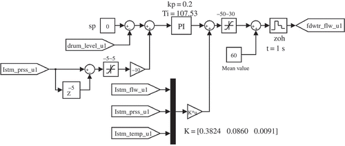
For safe operation of steam generators, the drum level has to be controlled by adjusting feedwater flow rate. Exceeding drum level from its limit may cause water carryover into the superheating sections or turbines, where decreasing drum level may also cause overheating of the water wall tubes. Both cases would result in severe damage or outage of either the boiler or the turbine. Here, a typical two-element control system is employed to adjust the drum level, which consists of feedback and feedforward control loops. The drum level (compensated by drum pressure signal) controller signal in addition to the measured value of steam flow rate (compensated by drum pressure and steam temperature signals) is deriving required feedwater flow rate (Figure A1).

Figure A1. Boiler feedwater controller.

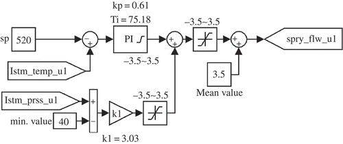
The final superheater temperature should also be maintained within the specified limits. A two-element control strategy is utilized to adjust the final superheater temperature. In this structure, steam pressure signal is considered as the transient correction signal in a feedforward controller. The summation of the output signals from the final superheater controller with feedforward signal is used to obtain the required water flow (Figure A2).

Figure A2. Superheater temperature controller.

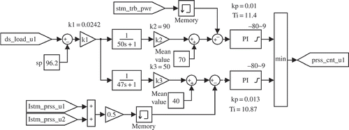
A dual-mode control system is supplied to regulate the speed (frequency) and acceleration of turbine during load demand changes. At steady-state conditions, the control system would be responsible for maintaining the boiler pressure at the set point. The output signals of the frequency and the pressure controllers are compared in a minimum selector block to override the corresponding control mode (Figure A3).

Figure A3. Unit load controller.

Appendix 2. The power characteristics of a gas turbine

The power characteristics of a Siemens V94.2 (also known as SGT5-2000E) gas turbine unit (Siemens AG, Erlangen, Germany) were presented by Ol'khovskii et al. [51], in which the relationship between the generated power and the fuel flow rate to the combustor section of a gas turbine was captured (Figure A4).

Figure A4. Dependence of the fuel flow rate on gas turbine power [36].

References

- Chen , K.Y. , Chen , L.S. , Chen , M.C. and Lee , C.L. 2011 . Using SVM based method for equipment fault detection in a thermal power plant . Comput. Ind. , 62 : 42 – 50 .
- Valdés , M. and Rapúm , J.L. 2001 . Optimization of heat recovery steam generators for combined cycle gas turbine power plants . Appl. Therm. Eng. , 21 : 1149 – 1159 .
- Gutiérrez Ortiz , F.J. 2011 . Modeling of fire-tube boilers . Appl. Therm. Eng. , 31 : 3463 – 3478 .
- Nanhua , Y. , Wentong , M. and Ming , S. 2006 . Application of adaptive grey predictor based algorithm to boiler drum level control . Energy Convers. Manage. , 47 : 2999 – 3007 .
- Flynn , M.E. and ’Malley , M.J. O . 1999 . A drum boiler model for long term power system dynamic simulation . IEEE Trans. Power Syst. , 14 : 209 – 217 .
- Chaibakhsh , A. , Ghaffari , A. and Moosavian , S.A.A. 2007 . A simulated model for a once-through boiler by parameter adjustment based on genetic algorithms . Simulat. Model. Pract. Theory , 15 : 1029 – 1051 .
- Lu , S. and Hogg , B.W. 2000 . Dynamic nonlinear modeling of power plant physical principles and neural networks . Int. J. Electr. Power. , 22 : 67 – 78 .
- Ljung , L. 2010 . Perspectives on system identification . Annu. Rev. Control , 34 : 1 – 12 .
- Rusinowski , H. and Stanek , W. 2010 . Hybrid model of steam boiler . Energy , 35 : 1107 – 1113 .
- Chawdhry , P.K. and Hogg , B.W. 1989 . Identification of boiler models . IEE Proc. Control Theory Appl. , 136 : 261 – 271 .
- Gao , L. and Dai , Y. 2011 . A new linear model of fossil fired steam unit for power system dynamic analysis . IEEE Trans. Power Syst. , 26 : 2390 – 2397 .
- Carrillo , C. , Feijóo , A.E. , Cidrás , J. and Medina , J.F. 2007 . A linear approach to study the influence of asynchronous wind parks on isolated networks . Electr. Power Syst. Res. , 77 : 1028 – 1037 .
- Doelman , R.B. and de Jager , A.G. 1995 . Dynamic modeling and simulation of a Cheng cycle cogeneration unit, IFAC Control of Power Plants and Power Systems Cancun , , Mexico
- Najimi , E. and Ramezani , M.H. 2012 . Robust control of speed and temperature in a power plant gas turbine . ISA Trans. , 51 : 304 – 308 .
- Sohn , J.J. and Seong , P.H. 2010 . A steam generator model identification and robust H∞ controller design with ʊ-gap metric for a feedwater control system . Ann. Nucl. Energy , 37 : 180 – 195 .
- Howard , R. and Cooper , D. 2010 . A novel pattern-based approach for diagnostic controller performance monitoring . Control Eng. Pract. , 18 : 279 – 288 .
- Simani , S. 2005 . Identification and fault diagnosis of a simulated model of an industrial gas turbine . IEEE Trans. Ind. Inf. , 1 : 202 – 216 .
- Ma , J. and Jiang , J. 2011 . Applications of fault detection and diagnosis methods in nuclear power plants: A review . Prog. Nucl. Energy , 53 : 255 – 266 .
- Prasad , G. , Swidenbank , E. and Hogg , B.W. 1998 . A local model networks based multivariable long-range predictive control strategy for thermal power plants . Automatica , 34 : 1185 – 1204 .
- Hametner , C. and Nebel , M. 2012 . Operating regime based dynamic engine modeling . Control Eng. Pract. , 20 : 397 – 407 .
- Peng , H. , Kitagawa , G. , Wua , J. and Ohtsu , K. 2011 . Multivariable RBF-ARX model-based robust MPC approach and application to thermal power plant . Appl. Math. Model. , 35 : 3541 – 3551 .
- Ayala , C.O. , Roca , L. , Guzman , J.L. , Normey-Rico , J.E. , Berenguel , M. and Yebra , L. 2011 . Local model predictive controller in a solar desalination plant collector field . Renew. Energy , 36 : 3001 – 3012 .
- Babuška , R. and Verbruggen , H. 2003 . Neuro-fuzzy methods for nonlinear system identification . Annu. Rev. Control. , 27 : 73 – 85 .
- Kalogirou , S.A. 2003 . Artificial intelligence for the modelling and control of combustion processes: A review . Prog. Energy Combust. , 29 : 515 – 566 .
- Jang , J.R. 1993 . ANFIS: Adaptive-network-based fuzzy inference . IEEE Trans. Syst. Man Cybern. , 23 : 665 – 685 .
- Fantoni , P.F. , Hoffmann , M.I. , Shankar , R. and Davis , E.L. 2003 . On-line monitoring of instrument channel performance in nuclear power plant using PEANO . Prog. Nucl. Energy , 43 : 83 – 89 .
- Vieira , J. , Morgado Dias , F. and Mota , A. 2004 . Artificial neural networks and neuro-fuzzy systems for modeling and controlling real systems: A comparative study . Eng. Appl. Artif. Intell. , 17 : 265 – 273 .
- Abdelazim , T. and Malik , O.P. 2005 . Identification of nonlinear systems by Takagi-Sugeno fuzzy logic grey box modelling for real-time control . Control Eng. Pract. , 13 : 1489 – 1498 .
- Kothamasu , R. and Huang , S.H. 2007 . Adaptive Mamdani fuzzy model for condition-based maintenance . Fuzzy Set. Syst. , 18 : 2715 – 2733 .
- Ghaffari , A. , Chaibakhsh , A. and Lucas , C. 2007 . Soft computing approach for modeling power plant with a once-through boiler . Eng. Appl. Artif. Intell. , 20 : 809 – 819 .
- Kishor , N. 2008 . Zero-order TS fuzzy model to predict hydro turbine speed in closed loop operation . Appl. Soft Comput. , 8 : 1074 – 1084 .
- Esen , H. and Inalli , M. 2010 . ANN and ANFIS models for performance evaluation of a vertical ground source heat pump system . Expert Syst. Appl. , 37 : 8134 – 8147 .
- da Costa , R.G. , de Abreu Mol , A.C. , de Carvalho , P.V.R. and Franklin Lapa , C.M. 2011 . An efficient Neuro-Fuzzy approach to nuclear power plant transient identification . Ann. Nucl. Energy , 38 : 1418 – 1426 .
- Peña , B. , Teruel , E. and íez , L.I. D . 2011 . Soft-computing models for soot-blowing optimization in coal-fired utility boilers . Appl. Soft Comput. , 11 : 1657 – 1668 .
- Fink , A. , öpfer , S. T and Isermann , R. 2003 . Nonlinear model-based control with local linear neuro-fuzzy models . Arch. Appl. Mech. , 72 : 911 – 922 .
- Johansen , T.A. and Foss , B.A. 1995 . Identification of non-linear system structure and parameters using regime decomposition . Automatica , 31 : 321 – 326 .
- Venkat , A.N. , Vijaysai , P. and Gudi , R.D. 2003 . Identification of complex nonlinear processes based on fuzzy decomposition of the steady state space . J. Process. Control , 13 : 473 – 488 .
- Guillaume , S. 2001 . Designing fuzzy inference systems from data: An interpretability-oriented review . IEEE Trans. Fuzzy Syst. , 9 : 426 – 443 .
- Habbi , H. , Kidouche , M. and Zelmat , M. 2011 . Data-driven fuzzy models for nonlinear identification of a complex heat exchanger . Appl. Math. Modell. , 35 : 1470 – 1482 .
- Gyun Na , M. , Weon Kim , J. and Hyuk Lim , D. 2007 . Prediction of residual stress for dissimilar metals welding at nuclear power plants using fuzzy neural network models . Nucl. Eng. Technol. , 39 : 337 – 348 .
- Jang , J.R. , Sun , C.T. and Mizutani , E. 1997 . Neuro-Fuzzy and Soft Computing , Upper Saddle River, NJ : Prentice Hall .
- Bezdek , J.C. , Ehrlich , R. and Full , W. 1984 . FCM: The fuzzy c-means clustering algorithm . Comput. Geosci. , 10 : 191 – 203 .
- Beliakov , G. and King , M. 2006 . Density based fuzzy c-means clustering of non-convex patterns . Eur. J. Oper. Res. , 173 : 717 – 728 .
- Pal , N.R. , Pal , K. , Keller , J.M. and Bezdek , J.C. 2005 . A possibilistic fuzzy c-means clustering algorithm . IEEE Trans. Fuzzy Syst. , 13 : 517 – 530 .
- Sivanandam , S.N. and Deepa , S.N. 2008 . Introduction to Genetic Algorithms , Berlin : Springer .
- Fleming , P.J. and Purshouse , R.C. 2002 . Evolutionary algorithms in control systems engineering: A survey . Control Eng. Pract. , 10 : 1223 – 1241 .
- Åström , K.J. and Bell , R.D. 2000 . Drum-boiler dynamics . Automatica , 3 : 363 – 378 .
- Gilman , G.F.J. 2010 . Boiler Control Systems Engineering , 2nd , Research Triangle Park , NC : ISA .
- Nelles , O. 2001 . Nonlinear System Identification , Berlin : Springer .
- Chaibakhsh , A. and Ghaffari , A. 2008 . Steam turbine model . Simulat. Model. Pract. Theory , 16 : 1145 – 1162 .
- Ol'khovskii , G.G. , Trushechkin , V.P. , Malakhov , S.V. and Ageev , A.V. 2003 . Thermoelectric power stations: Operating conditions of the V94.2 gas-turbine unit of the northwest cogeneration power plant . Power Technol. Eng. , 37 : 354 – 358 .