Aggregation of toxin-producing phytoplankton acts as a defence mechanism – a model-based study

Abstract

We propose a simple model of toxin-producing phytoplankton–zooplankton interactions in which the former is assumed to be able to detect the presence of zooplankton and to counteract it by forming patches and by releasing some toxic chemicals in the surrounding water. We observe that the formation of patch by the toxin-producing phytoplankton decreases the grazing pressure of zooplankton, resulting in stronger coupling between the interacting species determined by the fraction of the phytoplankton population that aggregates to form patches. Finally, the results were validated by comparing them with an alternative spatial model.

Keywords:

• Phytoplankton–zooplankton
• patch
• phase plane analysis
• stability criteria
• level of toxicity

1. Introduction

Toxic or otherwise, harmful algal blooms (HABs) are increasing in frequency worldwide [1,2] and have negative impact on aquaculture, coastal tourism and human health [3]. Many theories are available explaining the bloom phenomenon. Some of them use ‘top-down’ mechanism [4–7] to explain the bloom, that is, according to them, the occurrence of phytoplankton bloom depends on their grazing pressure, whereas some use ‘bottom-up’ mechanism [8–11], that is, the occurrence of bloom depends on the availability of the nutrient. Some researchers use simultaneous effect of both top-down and bottom-up mechanisms to explain the bloom phenomenon [12]. Quite a good number of studies [13–16] with the above-mentioned mechanisms have considered toxin-producing phytoplankton (TPP) as an important factor to explain the recurring bloom formation.

The toxin liberated by the phytoplankton may be regarded as an anti-grazing strategy [17]. Many researchers observe that the production of endo- or extracellular toxins is also a common property of several strains of pelagic primary producers, serving as an efficient grazer defence [18,19]. The evolution of toxins as a defence against the appropriate herbivores is often unclear and remains vigorously debated [20]. Most of these toxins are always present in the phytoplankton cells, but their concentration may go up because of the following chemical cues: (i) chemicals may be released from lysed cells (mechanical damage) of algal species that have not been in contact with a herbivore's digestive system [21]; (ii) herbivore-released chemicals that are produced by the herbivore and these chemicals are not related to feeding, for example, chemicals like sex pheromones or aggregation pheromones (intra-specific competition) [20] and (iii) specific chemical related directly to feeding, that is, when cells and/or their contents of the phytoplankton come into contact with the feeding apparatus and digestive system of the grazer [22]. However, still it is not clear whether the algal cells use them uniquely or in combination. It is also possible that there may exist some more possibilities for the toxin release.

The anti-grazing strategy is important not only for the existence of the phytoplankton species but also for many zooplankton species largely determined by the ways in which the species of phytoplankton can resist mutual extinction due to competition or persistence despite grazing pressure from zooplankton [23]. Among the various other anti-grazing strategies observed so far for phytoplankton, cell morphology [24], presence of gelatinous substances, or aggregate to form patches [25] and filamentous structures [26] are widely recognized. Because phytoplankton in the pelagic are small relative to their predatory enemies, they will not survive an encounter with a grazer without any anti-grazing strategy. Various studies have demonstrated that the formation of patches by green alga offers considerable protection against grazing by zooplankton [27]. Short-term grazing studies of zooplankton revealed that the rate of phytoplankton consumption decreases with increasing patch size, if the nutritional quality of algae is optimal [24]. The potent neurotoxin production by many microalgal species may have some direct or indirect effect in forming a patch and might be perceived by its grazer as group defence. Phytoplanktons may also form patches as an immediate response to some chemical stimulus released by the grazer [20].

The relation between defence strategies like patch formation and toxin release may give a possible answer to the evergreen crucial ecological question of why do many toxin-releasing microalgal species aggregate together to form patch leading to bloom. Toxic chemicals released through chemical signals by the phytoplankton patches may have indirect and cascading effects on the ecology of entire community and ecosystems. These signals between microbial predators and prey may contribute to food selection or avoidance and to defence, factors that probably affect trophic structure and algal blooms [17]. So the question is, in the above cases, do the level of toxicity and the fraction of the phytoplankton population that aggregates to form patches enhance the strength of coupling between interacting species? As such, this unknown mechanism offers considerable intellectual challenges to the theoretical and experimental ecologists. This article is devoted to understanding such dynamics by proposing a simple toxic phytoplankton–zooplankton system where the phytoplankton populations are assumed to aggregate into patches as a defence mechanism. In spite of the simple model structure and analysis, we obtained some interesting results that we later validated through an alternative reaction–diffusion equation, following the concepts of Petrovskii and Malchow [28] and Chaudhuri et al. [29].

The organization of this article is as follows: The mathematical model is dealt with in Section 2. The analysis is performed in Section 3. We propose an alternative spatial model in Section 4, and finally, the article ends with a conclusion in Section 5.

2. The basic mathematical model

The study of the defence mechanism through the formation of patches becomes more important if such patches have the ability to release toxin chemicals, like in the case of dinoflagellates [30]. The phytoplankton defence mechanism through the formation of patches was studied mainly using reaction–diffusion system. In population dynamics, this type of equations were first used by Segel and Jackson [31]. Later, Levin and Segel [32] suggested this scenario of spatial pattern formation for a possible origin of planktonic patchiness. After this, there were many articles that proposed reaction–diffusion model and the model was studied under different conditions [33–35]. For example, Serizawa et al. [36] studied a two-component diffusion model that can exhibit various types of spatial patterns including patchiness. Medvinsky et al. [37] also studied spatiotemporal complexity of plankton using reaction–diffusion equation and demonstrated that the diffusive instability can lead the system to spatiotemporal chaos, even though starting from simple initial conditions. There are many more articles, such as [38–40], that tried to capture the effect of phytoplankton patchiness using diffusion equation.

Although the simulation images created by the diffusion systems are closer to real patchiness patterns, solving those partial differential equations is not easy. Sometimes, the analytical solutions lead to complex relations. So, here, we proposed a simple mathematical model of TPP–zooplankton interactions in the presence of plankton patchiness using a system of ordinary differential equations (ODEs). In our predator–prey system, the prey as an act of defense group together and release toxin chemicals. The latter is assumed to diffuse in the surrounding water bed through the surface of the patch. This total defence strategy may involve some cost. For example, one distinct ecological cost of algal aggregation is limitation in photosynthesis and uptake of nutrient by reducing the available surface per volume [20]. But the literature on the costs of (inducible) defences is mixed. Some studies failed to detect cost in terms of nutrient or energy investment [41], whereas some found high costs [42,43] although most of them are found in terrestrial systems [20]. If there is any cost for the defence mechanism, then it is beneficial for the prey to activate its defence mechanism only in the presence of the predator. If there is no cost associated with the defence mechanism, then the benefit of the protection could be permanently enjoyed [44]. In this study, we assume no cost associated with the defence mechanism, and hence, we model it as a continuous function.

In this study, the space dimension is introduced in the model without using diffusion parameters. To capture the effect of phytoplankton patches on the zooplankton community, we propose a functional response that is not a monotonically increasing function of the prey density, but rather, it is only monotonically increasing up to a certain threshold density and then becomes monotonically decreasing. We also assumed that these patches have a negative impact on the growth of zooplankton.

Mathematically, let P(t) and Z(t) denote the phytoplankton (TPP) and zooplankton population sizes, respectively. The phytoplankton population is assumed to follow the law of logistic growth and the zooplankton consume phytoplankton for their growth. If the dynamics of the latter shows positive growth due to predation, then we must account for natural mortality and, finally, we include the poisoning effect. The sketch of the model is then

(1)

In the above equation, the poisoning effect needs to be coupled with the formation of the patches. We assume that the patch size is proportional to the phytoplankton density. This assumption is quite reasonable because many habitat fragmentation experiments show that the patch size is proportional to the population density [45]. For example, Bender et al. [46] show that patch size depends on population density. Root's [47] resource concentration hypothesis also shows that there is a positive relationship between patch size and population density. Suppose a fraction k () of the phytoplankton population aggregates to form N patches. For the predation term, the standard mass action incidence can easily be taken, over the fraction 1–k of the ‘free’ phytoplankton. We propose here a more complicated mechanism for the release of poison. Note that the population in each patch will be . Let us introduce a new parameter . If the 3D patch in the ocean can be assumed to be roughly spherical, its radius will be proportional to , so that its surface is proportional to

We assume that the phytoplankton can detect the presence of zooplankton and release the poison in self-defence, and this will leak into the surrounding water through the surface of the patch that is proportional to .

We are then led to the following equations:

(2)

where all parameters are non-negative, r is the growth rate, b is the phytoplankton's death rate, c is the predation rate and e is the conversion rate (assuming c ≥ e) and μ is the natural mortality rate of the zooplankton. The most important parameter is ρ that may be defined as the measure of the toxicity, which is directly proportional to the fraction of phytoplankton-forming patches and inversely proportional to the number of phytoplankton-forming patches.

2.1. Model validation

To analyse our proposed model close to real world scenario, we take parameter values from different literature sources (Table 1) and simulate our system (2) to compare it with the available literature on plankton dynamics [9]. For the above simulation, we considered hypothetical values for the parameters associated with the patch, varying them to see their effect on the system.

Table 1. The set of parameter values taken from different literature sources for our model

Parameters	Definition	Values considered	Range/value from literature
r	The growth rate of phytoplankton	1.5	1–2.9 [48, 49]
b	The death coefficient of phytoplankton	0.09	0.09–0.1 [50, 51]
c	The predation rate	0.14	0.04–0.17 [52]
e	The conversion efficiency of zooplankton	0.6 × c	(0.5–0.9)× c [52]
μ	The death rate of zooplankton	0.035	0.021–0.051 [48, 49, 52]
k	The fraction of phytoplankton aggregates	0.55	−
ρ	The degree of toxicity	0.0121	−
The units of P and Z are given in g m^−3 and the time is measured in days.

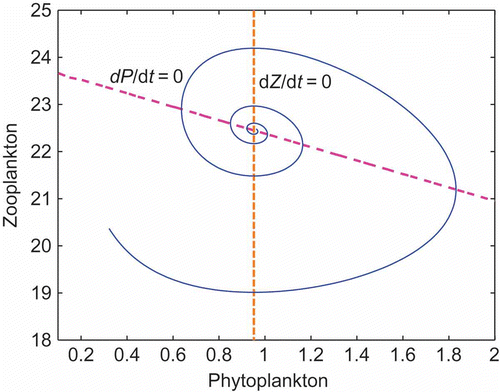
In [9], time-series data are produced from Peridinium gatunense phytoplankton blooms in Lake Kinneret, Israel, from 1970 to 1999. The phase plane analysis supports mechanistic grounds for such phytoplankton's behaviour. Such phase plane is symbolically sufficient to represent the plankton dynamics observed in the real world. Here, we reproduce their results with our system and experimentally estimate the parameter values, validating our proposed system. For the simulation, we used our own software written in Matlab 7.0. The phase plane is created using the free Matlab macro pplane6.m written by John Polking from Rice University, 1995, an interactive tool for studying planar autonomous systems of differential equations.

The time evolution of the simulation (Figure 1) shows the curves for Z against P with the Z–P nullclines and the obtained flow in the phase plane is divided in different stages as done by Huppert et al. [9], each with its own ecological meaning. The first stage is the lower left region ( and ) where the zooplankton population declines, and there is a slow constant increase in the TPP population P. P continues to grow until it crosses the threshold level () and the zooplankton population starts to grow (lower right region, the second stage). Next, the trajectory crosses the P nullcline (), where the TPP attains its maximum level P _max and moves into the upper right region ( and ) of the phase plane. In this region, zooplankton dramatically increases, whereas TPP starts to decrease. But this is the point at which TPP feels the lump of zooplankton population around itself and as a defence strategy starts releasing toxin chemicals [17]. Due to the action of these toxic chemicals, after some time, the zooplankton population starts to decline. This is observed in the figure, when the trajectory passes from the upper right into the upper left region and crosses the z nullcline (), where the zooplankton population attains its maximum level Z _max.

Figure 1. Phase plane diagram for the model (2). The phase plane may be used as a guide to trace out how the trajectory of the model changes with time as it is attracted towards equilibrium. A careful examination of and in the four regions shows that the trajectory must move counterclockwise through the phase plane in its approach to equilibrium.

3. Analysis of the model

3.1. Equilibrium points

The system (2) has only three equilibria : the origin E ₀, the boundary equilibrium point and another feasible non-boundary equilibrium E ₂. Its positive coordinates are found in the P–Z phase plane by solving the non-linear system and . Solving these two equations, we find , where P ₂ is the positive real root of the following cubic equation:

(3)

From Descartes' rule of sign, we observe that there exists at least one positive real root of the above equation (2)(2), and if that root is less than , then there exists a unique positive equilibrium point E ₂.

For example, with the parameter set considered in Table 1, Equation (3)(3) becomes

(4)

Equation (4)(4) has exactly one positive root, , and we obtain a unique interior equilibrium point .

3.2. Boundedness

Lemma 1:

Assume at first that the initial condition of Equation (2) (2) satisfies , then either (i) , for all t ≥ 0, and therefore, as , or (ii) there exists a t ₁ > 0 such that , for all t > t ₁. If instead , then , for all t ≥ 0.

Proof:

See Appendix.□

Lemma 2:

Letting , there is such that for any positive solution of the system (2) for all large t, we have , with .

Proof:

See Appendix.□

Theorem 1:

The set Ω, where

(5)

is a global attractor in and, of course, it is positively invariant.

Proof:

See Appendix.□

3.3. Local stability analysis

The Jacobian matrix of the system (2) has the form

(6)

At the origin, the eigenvalues are r, –μ showing its instability. At E ₁, we have the eigenvalues . Thus, E ₁ is conditionally stable if and only if . Finally, at the interior equilibrium E ₂, the eigenvalues are obtained as roots of the quadratic . Because and , we find that the Routh–Hurwitz criterion for stability is satisfied if , that is, if , which is equivalent to

(7)

Before proceeding further, let us recall for the benefit of the reader Dulac's criterion [53].

Dulac criterion.

Let us consider a system

where and . Further, , where E is a simply connected region of the plane. If there exists a function such that the divergence of the vector field p(x, y)g, that is,

is always of the same sign but not identically zero, then there is no periodic solution in the region E of the planar system.

Theorem 2:

The coexistence equilibrium E ₂ of the system (2) is globally asymptotically stable if the following conditions hold:

(8)

and

(9)

Proof:

The trajectories of (2) are bounded and the equilibrium point E ₀ is a saddle, the equilibrium point E ₁ is a repeller if and the interior equilibrium point E ₂ is locally asymptotically stable if . □

Now, we will test for the existence or non-existence of periodic solution around the positive equilibrium by using the Dulac criterion. Let and

Hence, there is no non-trivial positive periodic solution around the interior equilibrium point, proving the theorem.

Remark 1:

One can see from relation (9) that all the species coexist if the level of toxicity (ρ) falls below a certain threshold value depending on the fraction of phytoplankton that aggregates to form patches.

3.4. Numerical analysis

Our analytical result (see Theorem 2) ascertains that the system (2) is globally asymptotically stable around the positive interior equilibrium point and cannot explain the recurrent bloom phenomenon. We have seen from the experimentally obtained parameters that our system replicates plankton dynamics starting from bloom formation to termination. 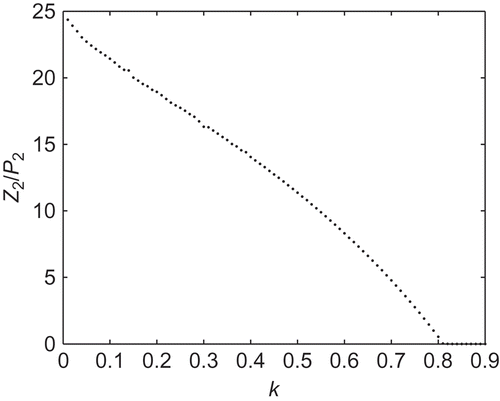To understand the role of defence mechanism like toxin chemicals and the patches in governing the plankton dynamics, we plotted the ratio of the zooplankton population at the interior equilibrium point E ₂ to the phytoplankton population at the same point against k, while all the other parameter values were kept fixed as in Table 1 except ρ. We vary both ρ and k in such a way that the number of patches N remains the same, here N = 3. The system (2) is numerically integrated using the built-in MATLAB function ode45, and after integration, we collected the final steady-state values for different combinations of ρ and k and plotted those values in the ρ–k space.

We observe the following values: for k = 0.01, the ratio is , and for k = 0.79, it is (Figure 2). Finally, when k crosses some critical value k_c , here k_c  = 0.82, the ratio tends to 0, which means that there is a huge increase in the phytoplankton population with respect to the zooplankton population. Thus, if the fraction of TPP population aggregating to form patches is small, it is easy for the zooplankton population to survive. But if the fraction of the phytoplankton population aggregating to form patches is larger, then there is a huge increase in the size of the phytoplankton population with respect to the zooplankton population. Thus, we may conclude that the formation of patches acts as a defence mechanism for the phytoplankton population, but the fraction of phytoplankton aggregating to form patches must not exceed a certain critical point.

Figure 2. The ratio of Z ₂ (the value of Z at the equilibrium point E ₂) to P ₂ (the value of P at the equilibrium point E ₂) with k is varied.

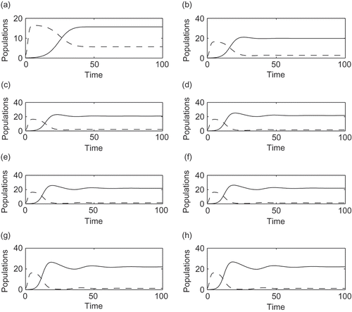
In the above simulation, we have considered a fixed number of patches (N = 3). It is interesting to see what happens to the value of the equilibrium point E ₂, when the number of patches N changes. To observe the role of N, we vary N and also ρ so that N always remains an integer, retaining the same other parameter values as in Table 1. For the numerical integration, we used the Matlab built-in function ode45 and plotted the time series for different values of N. We observe that Z ₂/P ₂ attains the smallest value for N = 1 (see Figure 3). Thus, when the TPP forms only one single patch, it is difficult for the zooplankton species to survive. But with an increasing number of patches, there is an increase in the size of the zooplankton population. Note that clearly the patch size reduces when their number increases, because we assumed a phytoplankton population of fixed size. Thus, if the number of patches is larger, it helps the zooplankton population to survive. Finally, when the value of N is increased beyond a certain threshold value, here N = 8, we observe only small changes in the values of E ₂, that is, the values of P ₂ and Z ₂ almost remain the same.

Figure 3. The dynamical behaviour of both populations for different values of N. ‘—’ denotes zooplankton population and ‘- - -’ denotes TPP population. (a) n = 1, P ₂ = 5.6684, Z ₂ = 15.7121; (b) n = 2, P ₂ = 2.787, Z ₂ = 19.8281; (c) n = 3, P ₂ = 2.1032, Z ₂ = 20.8057; (d) n = 6, P ₂ = 1.5276, Z ₂ = 21.6418; (e) n = 8, P ₂ = 1.3980, Z ₂ = 21.8380; (f) n = 10, P ₂ = 1.3228, Z ₂ = 21.9538; (g) n = 12, P ₂ = 1.2729, Z ₂ = 22.0318; (h) n = 15, P ₂ = 1.2225, Z ₂ = 22.1117.

4. A space-dependent model

From our previous model, we obtained a relation between the percentage and the size of phytoplankton aggregation and survival of the plankton population. Now to see the robustness of our results from the simple model, we propose and study a spatial version of our system (2) in which the patch formation is absent, in order to compare the previous results. This constitutes an important validation of our results, in view of the fact that we formulate a simple model to study a very complicated dynamics. If our result does not change much in the diffusion model, then we can claim that our proposed lumped parameter model can adequately capture the complex dynamics associated with the phytoplankton aggregation mechanism.

We explicitly incorporate diffusion in our model without phytoplankton aggregation. We introduce diffusion in our model followed in [28,29]. Mathematically, in our new system, we replace the term by θP, where θ represents the degree of toxicity, and we also of course drop the term k associated with the aggregation. Moreover, in the original model, we assumed that phytoplankton aggregates, but no aggregation was assumed for zooplankton. Here, we will assume spatial changes in both the species. Thus, a spatial analogue of the model (2) is presented here below:

(10)

where D ₁ and D ₂ represent the diffusion coefficients of P and Z, respectively. It is written in one dimension, but the extension to two dimensions is straightforward.

Let γ represent a suitable spatial domain in one or two dimensions as the case considered suggests. For the system (10) in the one-dimensional domain γ, we take the following initial conditions:

and the zero-flux boundary condition:

This means that no external input occurs across the boundary of these populations.

4.1. Model analysis

There are three equilibrium points for the model (10) in the absence of diffusion, out of which two are same as obtained from Equation (2)(2), that is, the origin E ₀ = (0,0) and the axial equilibrium point . The third equilibrium point is the coexistence point denoted by .

Denoting the general uniform steady state (USS) of the model (10) by , we investigate perturbations of the following form:

where l > 0 is the wave number of the spatial perturbation and λ > 0 is the time evolution rate.

By substituting these expressions in Equation (10)(10) and differentiating (using the fact that represents a steady state), we obtain the following differential equations:

After linearization, we seek the system's equilibria. The problem is then reduced to an eigenvalue problem in the parameter λ for the following matrix at the generic USS :

(11)

Its eigenvalues will thus provide the needed time dependency λ.

The eigenvalues for the plankton-free E ₀ are and . Hence, our diffusion model (10) showed that in the presence of diffusion, E ₀ is uniformly stable if and only if , that is, when the prey diffusion coefficients exceed a threshold, the system can collapse, wiping out both the populations. At E ₁, the eigenvalues are and . So, the system is stable around E ₁ if and only if . Thus, the condition for the stability of in the presence of diffusion (obtained from the diffusion model (10)) is similar to what we observed from the original model. Thus, the diffusion model does not change the result related to the preservation of phytoplankton and the washing out of the zooplankton from the system.

For the interior equilibrium point, E*, the eigenvalues are obtained as roots of the quadratic

(12)

where and if . Thus, from the Routh–Hurwitz criterion, the system shows stability in the presence of diffusion if . Hence, the system (10) does not show diffusive instability around E* (see Figure 4) and the conditions are almost the same as obtained from Equation (2)(2). In both the models, we observed that for the stability of coexistence equilibrium, the degree of toxicity has to be less than some threshold values.

Figure 4. Biomass distribution of phytoplankton and zooplankton over time and space for the model (10) for D ₁ = 10 and D ₂ = 2 with other parameter values from Table 1. Here, the value of θ is same as ρ. For this parameter set, the non-diffusive system shows stable coexistence. Here .

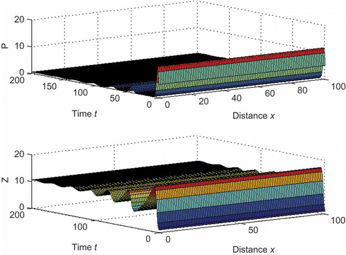
To observe the turbulence effect in our system, we consider the same diffusion rate for both the species as done by Petrovskii and Malchow [28]. Thus, if we consider the mixing due to turbulence, the condition for the stable coexistence of the species becomes , where D is the diffusion coefficient. Here, we have not considered the effect of turbulence explicitly because our model describes the general path size, whereas turbulence mainly controls the small-scale plankton patches, which are of size less than 100 m [28,54,55].

We can now summarize the whole discussion into the following remark:

Remark 2:

The stability properties of all the steady states of the system (10), except the trivial equilibrium point, remain almost the same as observed for the original model (2). The trivial steady state that is unstable in the original model is instead conditionally stable in the diffusion model.

5. Conclusion

Our proposed model assumes that the TPP population aggregates to defend itself from the zooplankton predation. This is well in accordance with results showing that the phytoplankton population forms patches to protect itself from grazers [30]. The coupled defence mechanism through patching and poison release results in the coexistence of the interacting species. Huisman and co-workers [56–58] have used the species coexistence to explain biodiversity and the plankton paradox. Our observations also indicate that there is a threshold in the number of patches enhancing the coupling strength of interacting species. Patch formation is important for the existence of the phytoplankton, but for zooplankton's survival, the patch size should not be large. So, to maintain biodiversity, phytoplankton needs to gather in small patches.

As discussed earlier, the common practice of mathematically capturing the effect of phytoplankton patchiness is through diffusion equations [38–40]. Researchers have used spatial models based on diffusion equations to find the critical length scales of phytoplankton patchiness in terms of phytoplankton growth and herbivore grazing [59]. Our simple model also provides a good explanation for the relation between the percentage and the size of the phytoplankton aggregation and the survival of the plankton population. Moreover, we observed that the incorporation of reaction–diffusion in the proposed model does not change the basic nature of the system's behaviour, except that there is a chance of total extinction if the prey diffusion is sufficiently high, larger than a certain threshold directly proportional to the phytoplankton reproduction rate.

Although we have proved the robustness of our results under diffusion mechanisms by using a simple reaction–diffusion system, the proposed model can be improved in a number of ways. For example, we could consider a more complex functional response to capture parameters like the saturation effect. We already mentioned that the activation of defence strategy is not clear, and here, we assumed a continuous function, but one could also take a step function to capture the discontinuity and compare the result with this study. In this study, we have ignored the explicit effect of turbulence. Turbulence has its own importance in these studies, because it quickly disrupts patches in nature, certainly preventing them from behaving like perfect spheres. More importantly, turbulence actively prevents group defence from being possible. It is observed that under active turbulence, not only the size and the shape of the patches change but also the spacing between patches get modified [60]. Finally, one can also consider separating the phytoplankton present outside the patch from the one inside the patch. Recent studies showed that the growth of a phytoplankton, grazing pressure and even nutrient availability is different for the inner and outer layers in a patch [61]. In this model, there is no term for zooplankton feeding inside and outside of patches. To obtain a more realistic model, separate equations for phytoplankton inside and outside of patches and for zooplankton inside and outside of patches could be formulated.

Although the proposed model can be extended and improved by the above modifications, we believe that increasing the complexity of the model will not change the basic results. We already observed this fact using the simple reaction–diffusion scheme in comparison with the lumped parameter model. We also believe that our study will open new door for the plankton ecologists to relate plankton survival with patch size and the fraction of population that aggregates to form patches.

Acknowledgements

The authors are thankful to the learned reviewers for their useful suggestions and comments. The authors also thank Dr. Sanjay Chaudhuri for providing the initial Matlab code for the diffusion model. The work of Samrat Chatterjee was partially supported by MIUR Bando per borse a favore di giovaniricercatori indiani and the work of Joydev Chattopadhyay was partially supported by the MAE Indo-Italian program of cooperation in Science and Technology, ‘Biomedical Sciences’.

Notes

Present address: Immunology Group, International Centre for Genetic Engineering and Biotechnology, Aruna Asaf Ali Marg, New Delhi-110067, India.

Appendix

Let us first recall (without proof) the Barbălat's [62] lemma:

Let g be a real-valued differentiable function defined on the half line . If (i) and (ii) g′(t) is uniformly continuous for t > a, then .

Proof of Lemma 1:

With the help of a Barbălat's lemma, one can easily prove the lemma and, hence, the proof is omitted.

Proof of Lemma 2:

Set . Calculating the derivative of W along the solutions of system (2), we find for t > t*

Taking , we get

It is clear that the right-hand side of the above expression is bounded. Thus, there exists a positive constant M such that for all large t. The assertion of lemma 1 now follows from the ultimate boundedness of P.

Proof of Theorem 1:

Due to Lemmas 1 and 2 for all initial conditions in such that does not belong to Ω, either there exists a positive time, say T, , such that the corresponding solution int Ω for all t > T, or the corresponding solution is such that as . But E ₁ is at the boundary of Ω, that is, , where ∂Ω represents the boundary of Ω. Hence, the global attraction of Ω in has been proved.

Assume now that int Ω. Then, Lemma 1 implies that for all t > 0, and also by Lemma 2, we know that for all large t. Finally, note that if , because or or both, then still the corresponding solutions must immediately enter int Ω or coincide with E ₁.

References

- Hallegraeff , G.M. 1993 . A review of harmful algal blooms and their apparent global increase . Phycologia , 32 : 79 – 99 .
- Smayda , T.J. 1989 . “ Primary production and the global epidemic of phytoplankton blooms in the sea: A linkage? ” . In Noval Phytoplankton Blooms: Causes and Impact of Recurrent Brown Tides and Other Unusual Blooms , Edited by: Cosper , E.M. 449 – 483 . Berlin : Springer Verlag .
- Anderson , D.M. , Kaoru , Y. and White , A.W. 2000 . Estimated Annual Economic Impacts form Harmful Algal Blooms (HABs) in the United States Sea , Woods Hole , MA : Woods Hole Sea Grant .
- Clother , D.R. and Brindley , J. 1999 . Excitabilty of an age-structured plankton ecosystem . J. Math. Biol , 39 : 377 – 420 .
- Edwards , A.M. and Brindley , J. 1999 . Zooplankton mortality and the dynamical behaviour of plankton population models . Bull. Math. Biol , 61 : 303 – 339 .
- Pitchford , J.W. and Brindley , J. 1999 . Iron limitation, grazing pressure and oceanic high nutrient-low chlorophyll (HNLC) regions . J. Plank. Res , 21 : 525 – 547 .
- Truscott , J.E. and Brindley , J. 1994 . Ocean plankton populations as excitable media . Bull. Math. Biol , 56 : 981 – 998 .
- Chan , T.U. , Robson , B.J. and Hamilton , D.P. 2003 . Modelling phytoplankton succession and biomass in seasonal West Australian estuary . Verh. Int. Ver. Limnol , 28 ( 2 ) : 1086 – 1088 .
- Huppert , A. , Blasius , B. and Stone , L. 2002 . A model of phytoplankton blooms . Amer. Natur , 159 : 156 – 171 .
- Robson , B.J. and Hamilton , D.P. 2004 . Three-dimensional modelling of a Microcystis bloom event in the Swan River estuary . Ecol. Model , 174/1–2 : 203 – 222 .
- Segal , R. , Waite , A.M. and Hamilton , D.P. 2006 . Transition from planktonic to benthic algal dominance along a salinity gradient . Hydrobiologia , 556 : 119 – 135 .
- Pal , S. , Chatterjee , S. and Chattopadhyay , J. 2007 . Role of toxin and nutrient for the occurrence and termination of plankton bloom – Results drawn from field observations and a mathematical model . Biosystems , 90 ( 1 ) : 87 – 100 .
- Burkholder , J.M. , Noga , E.J. , Hobbs , C.W. , Glasgow , H.B. Jr. and Smith , S.A. 1992 . New “phantom” dinoflagellate is the causative agent of major estuarine fish kills . Nature , 358 : 407 – 410 .
- Burkholder , J.M. , Hobbs , C.W. and Glasgow , H.B. Jr. 1995 . Distribution and environmental conditions for fish kills linked to a toxic ambush-predator dinoflagellate . Mar. Ecol. Prog. Ser , 124 : 43 – 61 .
- Fehling , J. , Davidson , K. and Bates , S.S . 2005 . Growth dynamics of non-toxic Pseudo-nitzschia delicatissima and toxic P. seriata (Bacillariophyceae) under simulated spring and summer photoperiods . Harmful Algae , 4 : 763 – 769 .
- Noga , E.J. , Smith , S.A. , Burkholder , J.M. , Hobbs , C.W. and Bullis , R.A. 1993 . A new ichthyotoxic dinoflagellate: Cause of acute mortality in aquarium fishes . Vet. Rec , 133 : 48 – 49 .
- Watanabe , M.F. , Park , H.D. and Watanabe , M. 1994 . Composition of Microcystis species and heptapeptide toxins . Verh. Int. Verein. Limnol , 25 : 2226 – 2229 .
- Lampert , W. 1987 . Feeding and nutrition in Daphnia . Mem. Ist. Ital. Idrobiol , 45 : 143 – 192 .
- DeMott , W.R. and Moxter , F. 1991 . Foraging on cyanobacteria by copepods: Responses to chemical defenses and resource abundance . Ecology , 72 : 1820 – 1834 .
- Van Donk , E. , Ianora , A. and Vos , M. 2011 . Induced defenses in marine and fresh water phytoplankton: A review . Hydrobiologia , 668 : 3 – 19 .
- Guisande , C. , Frangόpulos , M. , Caroteuto , Y. , Maneiro , I. , Riveiro , I. and Vergara , A.R. 2002 . Fate of paralytic shellfish poisoning toxins ingested by the copepod Acartia clausi . Marine Ecol. Prog. Ser , 240 : 105 – 115 .
- Stabell , O.B. , Ogbebo , F. and Primicerio , R. 2003 . Inducible defences in Daphnia depend on latent alarm signals from conspecific prey activated in predators . Chem. Sens , 28 : 141 – 153 .
- Mayeli , S.M. , Nandini , S. and Sarma , S.S.S. 2004 . The efficacy of Scenedesmus morphology as a defense mechanism against grazing by selected species of rotifers and cladocerans . Aqua. Ecol , 38 : 515 – 524 .
- Hessen , D.O. and Van Donk , E. 1993 . Morphological changes in Scenedesmus induced by substances released from Daphnia . Arch. Hydrobiol , 127 : 129 – 140 .
- Lampert , W. 1987 . Laboratory studies on zooplankton-cyanobacteria interactions . N.Z. J. Mar. Freshwater Res , 21 : 483 – 490 .
- Lynch , M. 1980 . Aphanizomenon blooms: Alternate control and cultivation by Daphnia pulex . Am. Soc. Limnol. Oceanogr. Spec. Symp , 3 : 299 – 304 .
- Donk , V.E. , ürling , M. L and Lampert , W. 1999 . “ Consumer-induced changes in phytoplankton: Inducibility, costs, benefits and impacts on grazers ” . In The Ecology and Evolution of Inducible Defenses , Edited by: Tollrian , R. and Harvell , C.D. 89 – 103 . Princeton , NJ : Princeton University Press .
- Petrovskii , S.V. and Malchow , H. 2001 . Wave of chaos: New mechanism of pattern formation in spatio-temporal population dynamics . Theor. Population Biol , 59 : 157 – 174 .
- Chaudhuri , S. , Chattopadhyay , J. and Venturino , E. 2012 . Toxic phytoplankton-induced spatiotemporal patterns . J. Biol. Phys , 38 : 331 – 348 .
- Smayda , T.J. and Shimizu , Y. , eds. 1993 . “ Toxic phytoplankton blooms in the sea ” . In Dev. Mar. Biol. 3 , 210 – 211 . New York : Elsevier Science . Limnol. Oceanogr. 39 (l) (1994)
- Segel , L.A. and Jackson , J.L. 1972 . Dissipative structure: An explanation and an ecological example . J. Theor. Biol , 37 : 545 – 559 .
- Levin , S.A. and Segel , L.A. 1976 . Hypothesis for origin of planktonic patchiness . Nature , 259 : 659
- Hillary , R.M. and Bees , M.A. 2004 . Patchiness . Phys. Rev. E , 69 ( 3 ) : 031913
- Malchow , H. 1993 . Spatio-temporal pattern formation in nonlinear nonequilibrium plankton dynamics . Proc. Roy. Soc. Lond. B , 251 : 103 – 109 .
- Upadhyay , R.K. , Kumari , N. and Rai , V. 2009 . Wave of chaos in a diffusive system: Generating realistic patterns of patchiness in plankton-fish dynamics . Chaos Soliton. Fract , 40 : 262 – 276 .
- Serizawa , H. , Amemiya , T. and Itoh , K. 2008 . Patchiness in a minimal nutrient – Phytoplankton model . J. Biosci , 33 ( 3 ) : 391 – 403 .
- Medvinsky , A.B. , Petrovskii , S.V. , Tikhonova , I.A. , Malchow , H. and Li , B.L. 2002 . Spatiotemporal complexity of plankton and fish dynamics . SIAM Rev , 44 ( 3 ) : 311 – 370 .
- Abraham , E.R. 1998 . The generation of plankton patchiness by turbulent stirring . Nature , 391 ( 6667 ) : 577 – 580 .
- Neufeld , Z. , Haynes , P.H. , Garçon , V. and Sudre , J. 2002 . Ocean fertilization experiments may initiate a large scale phytoplankton bloom . Geophys. Res. Lett , 29 ( 11 ) : 1 – 4 .
- Tzella , A. and Haynes , P.H. 2007 . Small-scale spatial structure in plankton distributions . Biogeosciences , 4 ( 2 ) : 173 – 179 .
- Van Lurling , D. 2000 . Grazer-induced colony formation in Scenedesmus: Are there costs to being colonial? . Oikos , 88 : 111 – 118 .
- Strauss , S.Y. , Rudgers , J.A. , Lau , J.A. and Irwin , R.E. 2002 . Direct and ecological costs of resistance to herbivory . Trends Ecol. Evol , 17 : 278 – 285 .
- Cipollini , D. , Purrington , C.B. and Bergelson , J. 2003 . Costs of induced responses in plants . Basic Appl. Ecol , 4 : 79 – 89 .
- Tollrian , R. and Harvell , C.D. 1999 . The Ecology and Evolution of Inducible Defenses , 383 Princeton , NJ : Princeton University Press .
- J. Bowman, N. Cappuccino, and L. Fahrig, Patch size and population density: The effect of immigration behavior. Conserv. Ecol. 6 (1) (2002), p. 9. http://www.consecol.org/vol16/iss1/art9/ (http://www.consecol.org/vol16/iss1/art9/)
- Bender , D.J. , Contreras , T.A. and Fahrig , L. 1998 . Habitat loss and population decline: A meta-analysis of the patch size effect . Ecology , 79 : 517 – 533 .
- Root , R.B. 1973 . Organization of a plant-arthropod association in simple and diverse habitats: The fauna of collards (Brassica oleracea) . Ecol. Monogr , 45 : 95 – 120 .
- Fennel , K. , Losch , K. , Schroter , J. and Wenzel , M. 2001 . Testing a marine ecosystem model: Sensitivity analysis and parameter optimization . J. Marine Syst , 28 : 45 – 63 .
- Fashman , M.J.R. , Ducklow , H.W. and McKelvie , S.M. 1990 . A nitrogenbased model of plankton dynamics in the oceanic mixed layer . J. Marine Res , 48 : 591 – 639 .
- Svirezhev , Y.U. , Krysanova , V.P. and Voinov , A.A. Mathematical modelling of a fish pond ecosystem . Ecol. Model , 21 ( 1983/1984 ) 315 – 337 .
- Serizawa , H. , Amemiya , T. and Itoh , K. 2010 . Sufficient noise and turbulence can induce phytoplankton patchiness . Nat. Sci , 2 : 320 – 328 .
- Dube , A. and Jayaraman , G. 2008 . Mathematical modelling of the seasonal variability of plankton in a shallow lagoon . Nonlinear Anal , 69 : 850 – 865 .
- Kot , M. 2001 . Elements of Mathematical Ecology , Cambridge : Cambridge University Press .
- Platt , T. 1972 . Local phytoplankton abundance and turbulence . Deep Sea Res , 19 : 183 – 187 .
- Powell , T.M. , Richerson , P.J. , Dillon , T.M. , Agee , B.A. , Dozier , B.J. , Godden , D.A. and Myrup , L.O. 1975 . Spatial scales of current speed and phytoplankton biomass fluctuations in Lake Tahoe . Science , 189 : 1088 – 1090 .
- Huisman , J. and Weissing , F.J. 2000 . Reply – Coexistence and resource competition . Nature , 407 : 694
- Irigoien , X. , Huisman , J. and Harris , R.P. 2004 . Global biodiversity patterns of marine phytoplankton and zooplankton . Nature , 429 : 863 – 867 .
- Stomp , M. , Huisman , J. , de Jongh , F. , Veraart , A.J. , Gerla , D. , Rijkeboer , M. , Ibelings , B.W. , Wollenzien , U.I.A. and Stal , L.J. 2004 . Adaptive 26 divergence in pigment composition promotes phytoplankton biodiversity . Nature , 432 : 104 – 107 .
- Wroblewski , J.S. and O'Brien , J.J. 1976 . A spatial model of phytoplankton patchiness . Mar. Biol , 35 ( 2 ) : 161 – 175 .
- Mitchell , J.G. , Yamazaki , H. , Seuront , L. , Wolk , F. and Hua , L. 2008 . Phytoplankton patch patterns: Seascape anatomy in a turbulent ocean . J. Mar. Syst , 69 : 247 – 253 .
- Menden-Deuer , S. and Fredrickson , K. 2010 . Structure-dependent, protistan grazing and its implication for the formation, maintenance and decline of plankton patches . Mar. Ecol. Prog. Ser , 420 : 57 – 71 .
- Barbălat , I. 1959 . Systemes d'equations diff´erentielles d'oscillation non lineares . Math. Pure Appl , 4 : 267