Predicting high-codimension critical transitions in dynamical systems using active learning

Abstract

Complex dynamical systems, from those appearing in physiology and ecology to Earth system modelling, often experience critical transitions in their behaviour due to potentially minute changes in their parameters. While the focus of much recent work, predicting such bifurcations is still notoriously difficult. We propose an active learning approach to the classification of parameter space of dynamical systems for which the codimension of bifurcations is high. Using elementary notions regarding the dynamics, in combination with the nearest-neighbour algorithm and Conley index theory to classify the dynamics at a predefined scale, we are able to predict with high accuracy the boundaries between regions in parameter space that produce critical transitions.

Keywords:

• dynamical systems
• Conley index
• machine learning
• combinatorial dynamics

1. Introduction

Critical scientific problems are increasingly marked by the need to understand the dynamical behaviour of complex systems. Merely decomposing a problem into isolated subsystems, and attempting to extrapolate the behaviour of the whole system from the steady-state behaviour of each subsystem is often insufficient. The importance of studying the dynamics of complex systems is exemplified by the wide range of fields in which such systems constitute major research foci [1,2]. Examples of complex systems include scale-free networks in fields ranging from biology and neuroscience to computer science and internet research [3,4]; analysis of high-dimensional models in ecology and physics [5–7]; and the study of atmospheric circulation ranging from small-scale theoretical studies [8] to the macro-scale models of global circulation. The need to study directly the entire aggregate system, instead of decomposing a system into its constituent parts is intuitively clear in climate change models: one is interested in the time-dependent trajectory of the entire planetary system over decades and centuries [9–11]. The mechanisms driving the climate are integrally coupled, making analysis via decomposition difficult or impossible [10,12–14].

A key component in the long-term behaviour of complex dynamical systems is a sensitive dependence on the parameters chosen for the model, as well as the initial conditions. Furthermore, for physical models, the parameter values are often only known approximately, and the amount by which they affect the system cannot be precisely determined. This introduces uncertainty in every step of the modelling process.

The classical dynamical system paradigm is to consider particular autonomous systems with one or two parameters, and study invariant sets which may be particularly sensitive to change in parameters. In the face of the aforementioned problems, this approach often falls short. Therefore, there is a need for conceptually new approaches to nonlinear dynamical systems with many parameters [9,11].

One exciting new approach backs away from the traditional concept of an invariant set as the principle object of study for a dynamical system and focuses instead on the related concept of a Morse set. Morse sets have the advantage that they are robust with respect to perturbations, including certain types of noise, while also being computationally tractable [15,16]. This robustness allows one to make statements about the qualitative behaviour of a system over a range of parameters. Morse sets are also naturally ordered by dynamics. The collection of Morse sets with the dynamics-compatible partial ordering is a Morse decomposition, and organizes the long-term behaviour of the dynamics. Additionally, Morse decompositions have a natural combinatorial representation as a directed graph, where the vertices correspond to the Morse sets and the edges represent the dynamics-compatible ordering. This object is the Morse graph and is a central object of this approach to dynamics [15,17].

This paper is organized as follows. In Section 2, we summarize the background necessary for constructing Morse graphs. We then show how the Morse graph approach can be used to construct a database of dynamical systems that can be queried in order to locate parameters at which global changes in dynamics occur. However, construction of the database at a reasonable grid size in high-dimensional parameter spaces is computationally expensive and inherently suffers from the curse of dimensionality. In Section 3, we describe a novel machine-learning approach to the construction of such a database that builds on the work of Arai et al. [15,18]. Sections 4 and 5 describe the model with which we demonstrate our algorithm as well as the learning algorithms used to build the database. In Section 6, we demonstrate that by incorporating our learning algorithms, we are able to compute the Morse graphs of as few as 20% of the grid elements in a discretized parameter space, while correctly classifying the dynamics of over 98% of parameter space.

2. Conley–Morse database

In this section, we provide a brief review on the fundamentals necessary to construct a database of global dynamics. The reader is referred to [15,19] for further details.

2.1. Preliminaries

Instrumental to this work is the Conley index theory, an important tool for analysing the dynamics of both continuous and discrete dynamical systems. In particular, the Conley index can be used to find stationary, periodic or heteroclinic orbits or to prove the chaotic behaviour of dynamical systems. More specifically, the Conley index is an algebraic topological invariant of isolated invariant sets.

To simplify our exposition, we will focus primarily on the combinatorial aspects of the database, and refrain from speaking at length on algebraic topology. Furthermore, as our experimental model is a map, we will restrict our exposition to the discrete case, primarily following the outline of [15]. Further details on Conley index theory can be found in [16,19].

Let be a map on a locally compact metric space X and a parameter space Λ that is a compact, locally contractible, connected metric space. At a particular parameter value λ, we will sometimes denote f(x, λ) as f_λ(x).

The fundamental mathematical structures in the study of dynamical systems are invariant sets. A subset Z ⊂ X is invariant at the parameter λ ⊂ Λ if . When considering computational dynamics, it is important to note that we cannot compute at each parameter independently, and therefore are most interested in sets which are invariant with respect to a subset of the parameter space.

We use the notation for the extension of f to include the parameters as explicit variables, i.e. . For a subset of the parameter space , let denote the restriction of F to . For a set , we denote its restriction to Λ₀ by . We say a set is invariant over Λ₀ if .

Within the database framework, the primary use of Conley index theory is to identify a finite collection of invariant sets which determine the global behaviour of the dynamics within a particular compact set of parameter values. To this end, we will review two essential structures: isolating neighbourhoods and isolated invariant sets.

Definition 2.1:

An isolating neighbourhood is a compact set such that its maximal invariant set lies in its interior, i.e.

where int(·) denotes the interior of a set. An invariant set is an isolated invariant set if for some isolating neighbourhood N.

The advantage of our focus on isolating neighbourhoods is that they are robust to perturbations. This fact is captured in the notion of continuation, which states that given an isolating neighbourhood, N, then N will also serve as an isolating neighbourhood for a map with sufficiently close parameters [16]. For our purposes, the most important feature of isolating neighbourhoods is that they are readily computable [20].

2.2. Morse decompositions

We first introduce some elementary concepts from the theory of dynamical systems. A more in-depth treatment can be found in [21].

Definition 2.2:

Consider x₀ ∈ X. The ω-limit set of x₀ is

while the α-limit of x₀ is

where cl(·) denotes set closure.

The following definition is central to the mathematical and computational aspects of this work. Morse decompositions provide a coarse, global description of the dynamics on .

Definition 2.3:

A Morse decomposition of is a finite collection of disjoint isolated invariant subsets of indexed by the set , i.e.

On the index set , there exists a strict partial order such that for all there exist such that and . The sets are known as Morse sets.

It is worth noting that while Morse sets may not be preserved under perturbation, the decomposition itself is robust in the sense that the decomposition and the associated isolating neighbourhoods are preserved. In particular, Morse decompositions inherit the continuation property of isolating neighbourhoods. From a computational viewpoint, since is a partially ordered set, a Morse decomposition can be naturally represented as a Morse graph, a directed acylic graph with vertice and edges .

Morse graphs are the fundamental objects of the Conley–Morse database. Morse graphs provide a natural combinatorial representation for the dynamical system which can be compared in order to detect changes in the dynamics across regions in parameter space.

2.3. An example

To motivate our methods, we will illustrate some aspects of our approach on the following model of spruce budworm populations, originally introduced by Ludwig [22]. The model is a classical example of insect outbreak as spruce budworm can defoliate the balsam fir, leading to potentially major environmental issues in eastern North America. We follow the exposition of Murray [23], with the budworm population dynamics given by the following equation:

Here, r_B is the linear birth rate of the budworm and K_B is the carrying capacity of the environment (associated with the density of foliage available on the trees). The predation term, , is that originally suggested by Ludwig for its qualitative behaviour (predation saturates for large enough N).

We consider the nondimensional quantities:

which leads to the following nondimensionalized equation:

The system now has only two parameters, r and q, which are dimensionless quantities.

The steady states of the system correspond to the solutions of

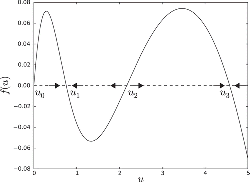
A conventional dynamical analysis reveals that either one or three solutions exist, depending upon the parameters, r and q [23]. For instance, for appropriate values of r and q, the phase portrait has three equilibria as shown in Figure 1.

Figure 1. Dynamics for choice of (q, r) exhibiting three steady states.

The smaller stable equilibrium, u₁, is the refuge equilibrium while the stable equilibrium, u₃, is the outbreak equilibrium. The unstable equilibrium at the origin, u₀, corresponds to extinction.

While equilibria in this particular example can be computed analytically, more complicated invariant sets in high-dimensional spaces are, in general, not accessible to analytic methods. Furthermore, small perturbations can lead to a cascade of changes in the internal structure of these sets, while the overall shape may remain the same. Therefore, we focus on isolated invariant sets, which are, by definition, stable under perturbations and their associated isolating neighbourhoods are readily computable. In our simple example where the phase space is one-dimensional, isolating neighbourhoods are intervals whose boundary does not intersect an invariant set, i.e. an equilibrium. In Figure 2, we depict a one-parameter family of phase portraits parameterized by q, for a fixed r = 0.535. The curve is the set of zeros for . The intervals represent isolating neighbourhoods at a given value of r and q with nontrivial isolated invariant sets which in this case are equilibria. Similar intervals isolate the equilibrium at u₀ = 0 which we chose not to depict for the sake of clarity.

Figure 2. Isolating neighbourhoods for equilibria u₁, u₂, u₃ from Figure 1 as a function of parameter q and a fixed r. The isolating neighbourhood for u₀ is omitted for clarity.

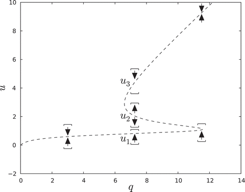
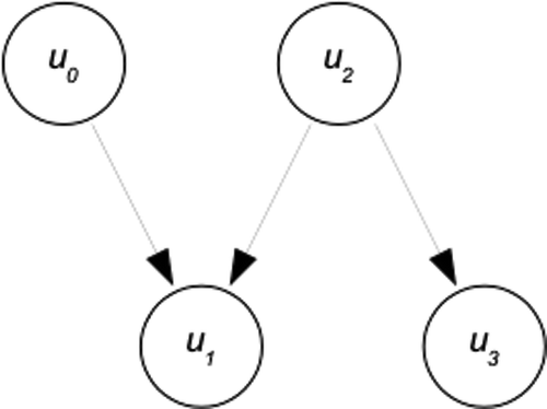
We now concentrate on the value of q = 7.5. At this value, there are three isolated invariant sets. The flow between the neighbourhoods that isolate u₀, u₁, u₂ and u₃ induce a flow-defined partial order on these neighbourhoods. Isolated invariant sets, together with this partial order, define a Morse decomposition of the invariant set M (S_q) at q = 7.5. This information is represented combinatorially in terms of a Morse graph, depicted in Figure 3.

Figure 3. Morse graph for Morse decomposition for M (S_q), q = 7.5, see Figure 2. (u₀ has been included.)

The classical bifurcation theory shows that the budworm model exhibits hysteresis which is a basis for predictions of outbreak dynamics [23]. Figure 4(a) depicts the set of equilibria as a function of both parameters, and Figure 4(b) shows the parameter region where three nonzero equilibria coexist. In the language of Morse decompositions, in the shaded region, the Morse decomposition is that depicted in Figure 3, while outside of this region consists of two isolated invariant sets, one corresponding to u₀ and the other to a stable equilibrium.

Figure 4. (a) Equilibria states in a general cusp catastrophe model. In the region of the fold, three equilibrium states exist. One equilibrium exists in other regions. The dashed vertical line shows the arrangement of the equilibria in phase space for an arbitrary pair of parameters (q, r) in the cusp region. The repeller and attractors in the Morse graph in Figure 3 correspond to u₁, u₂ and u₃. (b) Parameter space showing the projection of the folded region on the right.

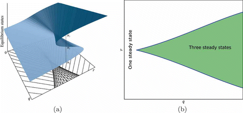
This example shows the key role of classifying regions of parameter space into different types of dynamics. Such an analysis can form a basis for interventions and control of the system to a desired regime. The database approach that we use in this paper, and describe in following sections, aims to compute a partitioning of the parameter space into regions with identical Morse decompositions. In particular, we emphasize that our techniques are amenable to computation. The emphasis on computability is essential as analytical techniques are often of limited use in large-size problems, found in real-world applications.

2.4. Combinatorial dynamics

In this section, we review precisely how Morse graphs are computed. From [15], a grid on a metric space Z is a collection nonempty compact subsets of Z with the following properties

2. G = cl(int(G)) for all

3. for all

4. If Y ⊂ Z is compact, then is finite

In the context of a grid, we define the support function | · | from subsets of to subsets of Z by . Further, given Y ⊂ Z, we define

For the rest of the paper, we denote by and the grids on phase space and parameter space, respectively.

We now discuss a method for exploring the dynamics of f computationally. A combinatorial multi-valued map assigns to each element a finite (and possibly empty) subset of as follows. It is defined as follows. Consider and its combinatorial enclosure formed by the collection of all grid elements such that . Then the multi-valued map is defined as

Furthermore, the combinatorial enclosure gives an outer approximation of f by defining

This provides rigorous bounds on the dynamics of f. An essential component of this approach is the use of interval arithmetic software to construct , providing a rigorous bound on any approximation error as well [24]. Efficient algorithms exist to compute isolating neighbourhoods and Conley indices from the combinatorial enclosure . Furthermore, is represented as a graph, opening up its analysis to efficient graph algorithms as well [19].

In order to construct Morse graphs, we first start with the recurrent set of , defined by

The recurrent set can be partitioned into equivalence classes called combinatorial Morse sets by the equivalence relation if and only if there exists a path in from G to H and a path in from H to G. This gives a strict partial order on the indexing set by setting p > _Qq if there exists , and a path from G to H in .

By construction, the combinatorial Morse decomposition can be represented by a directed graph. We define the Morse graph to be the acylic directed graph with vertices consisting of the elements of and the minimal set of directed edges (p, q) which generate p > _Qq under transitivity.

2.5. Comparing Morse graphs

We now review how to use Morse graphs to compare dynamics over different regions in parameter space. Suppose that for each Q in we have computed . In order to compare each MG, we define the clutching graph and clutching function.

Definition 2.4:

Consider where . The clutching graph is the bipartite graph with vertices and edges if .

If every vertex in in the clutching graph has a unique edge, then we define the clutching function by for each edge (p, q) of .

Consider and their corresponding Morse graphs , , where . If the clutching function ι is defined for the clutching graph , and ι gives a directed graph isomorphism from to , then we consider and to be equivalent. As in Arai et al. [2], we say that the equivalence classes of with respect to the transitive closure of this relation are continuation classes.

The purpose for requiring that ι defines a directed graph isomorphism as opposed to merely a bijection is that differences in the partial order may indicate differences in the dynamics. In [15] it is shown that if and belong to the same continuation class, then there is a path in parameter space along which the underlying Morse decompositions are related by continuation. However, compared to classical notions of equivalence, two Morse graphs belonging to the same continuation class is a relatively weak form of equivalence. In general, this is due to investigating the dynamics at the level of grid elements. We refer the reader to [15] for further elaboration.

The position we take in this paper is that continuation classes are a significant and useful notion for constructing a database of global dynamics. In other words, the database consists of a combinatorial representation of the set of continuation classes and their relative connectivity. This concept is formalized in an efficient manner in the following definition [15].

Definition 2.5:

The continuation graph of is a graph whose vertices are the continuation classes where is the set of parameter boxes associated with the k-th continuation class, and for some .

2.6. Conley–Morse database

We will now summarize the process to construct the complete database for a given dynamical system. The first step is to choose the resolution for the grids and , on the phase and parameter spaces, respectively. The next step is to construct the combinatorial multi-valued map on . Then the Morse graph must be determined for each . For each pair of adjacent grid elements, Q₀, Q₁ in the parameter space, the clutching graph must then be formed, with the clutching function ι tested to determine whether it defines a directed graph isomorphism.

Unfortunately, exhaustively computing upon parameter space in this fashion is very computationally demanding. In fact, the computational burden of producing the Conley–Morse database has inspired previous machine learning approaches [18]. We expand upon this work by introducing novel machine learning algorithms and ideas for approximating the database computation.

Now that we have introduced the Conley–Morse database, recall that in this paper, our focus is on predicting the locations of potential bifurcations. In the setting of the database, this corresponds to discerning the edges between regions of grid elements which belong to the same continuation class.

3. Learning the Conley–Morse database

As we want to refrain from computing the entire parameter space, we do not form the clutching graph to check the pairwise intersection of Morse sets in the phase space. Thus, we cannot assign the correct continuation classes for intersecting grid elements in parameter space. Instead, we define two grid elements to belong to the same equivalence class if there exists a directed graph isomorphism between their corresponding Morse graphs.

Definition 3.1:

Let G and H be directed graphs. A directed graph isomorphism between G and H is a bijection h that maps V (G) to V (H) and E (G) to E (H) such that each is mapped to .

For , we define if there exists a directed graph isomorphism between them. As a result of our changes to the Conley–Morse database framework, our equivalence classes are coarser than continuation classes. Nevertheless, we show that our algorithms still detect a significant portion of phase transitions.

4. Leslie model

We illustrate our approach on a nonlinear Leslie population model. This model and its relevance to population biology is discussed further in [25]. In the Leslie model, the population is partitioned into d generations, each with population , and an associated reproduction rate. The nonlinearity stems from the assumption that fertility decreases exponentially with the total size of the population.

For our experiments, we consider the two-generation Leslie model with a three-dimensional parameter space , given by:

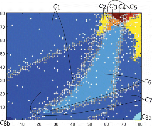
Mirroring [15], we select an 80 × 80 × 40 grid for the three-dimensional parameter space, which we label traditionally as x, y and z axes, respectively. Since in [15] they performed an exhaustive computation on this subset of parameter space, we are able to compare our weaker notion of equivalence with the result provided by their continuation classes. Fixing z, we obtain a brute-force, or ‘ground truth’, result without the use of learning algorithms, but with our notion of weaker equivalence. We compare this with the continuation class results from [15] in the continuation diagram in Figure 5. In the continuation diagram, regions of parameter space which are of the same colour correspond to a continuation or an equivalence class. For instance, one difference between our two notions of equivalence can be seen in the upper left region in Figure 5(b), which is detected to be of the same class as other regions of the same colour, whereas in Figure 5(a) the same region is distinguished from the others. However, in all of these figures, the colours are arbitrary, thus the difference in colour between Figure 5(a) and (b) is not representative of anything.

Figure 5. A slice of parameter space at z = 1. (a) Continuation classes from the original paper by Arai et al.; (b) Classes obtained without machine learning algorithms, but using the coarser notion of equivalence. Classes labels, C_*, correspond between (a) and (b) as well as to those in the figures below (colour online).

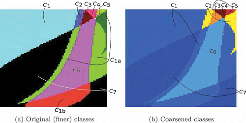
Recall that in Arai, a Morse graph is computed for each grid element . The clutching graph is then formed for all adjacent boxes , and the clutching function ι is tested to determine if it defines a directed graph isomorphism. The equivalence classes with respect to the transitive closure form the continuation classes. In the continuation diagram, grid elements of identical colours indicate that they belong to the same continuation classes.

In contrast, in Figure 5(b), we present classification using a coarser equivalence relationship, where two Morse graphs are equivalent if they are isomorphic. This represents our ‘ground-truth’ for classification. The boundaries between the clusters of identically coloured grid elements in parameter space are potentially critical transitions in the dynamical behaviour. It should be noted that while the Conley–Morse database results are rigorous at the pre-specified resolutions, the results depend upon resolution in both parameter space and phase space. For the purposes of this paper, our resolutions are identical to those in [15]. However, for future analysis, the efficiency of machine learning allows us to use much finer resolutions in both parameter and phase space.

5. Methodology

In this section, we provide a review of the requisite machine learning techniques, and give a description of our algorithms.

5.1. Active learning

Active learning is a form of supervised learning in which it is possible for the learning algorithm to perform interactive queries of the data in order to generate a training set [26,27]. The rationale for active learning is that a machine learning classifier can achieve greater accuracy with a smaller training set if it is allowed to choose which samples to learn from.

Active learning is primarily motivated by instances where labelling data is expensive. In the setting of predicting bifurcations, labelling data corresponds to computing Morse graphs. As this is one of the most computationally intensive parts of the construction of the Conley–Morse database, the active learning paradigm applies naturally to building the database.

The most popular form of active learning is uncertainty sampling, where samples are chosen based on where the classifier is least certain of classification. In other words, samples which change the potential classification by small amounts are of little value, whereas samples which can change the classification substantially are of high value.

In order to incorporate this philosophy into the framework of the Conley–Morse database, we rely on the continuation properties of the Morse graphs. We make a heuristic assumption that regions enclosed by grid elements with isomorphic Morse graphs likely belong to the same continuation class. As such, queries within such a region are thought to be of low value. In selecting a random query, an active learning subroutine decides whether the query is of high value, and if so, adds it to the training set. The goal of our active learning subroutine is to iterate this procedure in order to build up a small, yet informative training set.

5.2. Algorithmic preliminaries

The k-Nearest Neighbour (k-NN) classification algorithm is a well-established method for classifying or labelling objects based on the closest training examples in a feature space. For more detail, see [28].

For our purposes, the feature space is the discretized parameter space of a dynamical system. The class of a grid element Q₀ in the is the equivalence class to which the associated Morse graph belongs.

5.3. Delaunay triangulation

To interactively construct an effective training set, our goal is to choose a minimal number of informative samples. To do this, we consider the geometry of the current training set in parameter space, and accept queries from boundary regions.

In order to judge whether a query is in such a region, it is natural to turn to computational geometry. Our computational geometry approach is to consider the Delaunay triangulation of the elements of the current training set.

Definition 5.1:

A Delaunay triangulation for a set P of points in a plane is a triangulation such that no point in P is inside the circumcircle of any triangle in .

The benefit of the Delaunay triangulation is that it produces ‘fat’ simplices by maximizing the minimum angle of all the angles in the triangulation. Such triangles are more effective for our purposes. Using point location algorithms, it is straightforward to determine the location of the query in the triangulation, and compare Morse graphs of the vertices that make up the encompassing simplex. If the vertices of the encompassing simplex have isomorphic Morse graphs, the query is discarded as a low-information point, otherwise it is accepted into the training set. Computational geometry, in the form of the Voronoi diagram, has previously been used in conjunction with the nearest-neighbour classification algorithm [29]. However, our approach is disparate in that our active learning techniques are tailored to the dynamics rather than the classification algorithm.

The time complexity of the implemented Delaunay triangulation algorithm is in the planar case, while the complexity of the point location algorithm is [30]. We consider this an acceptable computational overhead in order to generate an effective training set. However, for dimension d, the complexity of the Delaunay triangulation is [30]. Above two dimensions this overhead is quite large, and this approach becomes infeasible for large training sets. In order to circumvent this problem, we consider two different directions. First, we split the three-dimensional domain into slices along the z axis. Second, we develop a similar active learning algorithm that performs at a lower complexity.

Table

AlgorithmD
1 M ← m     ▹ Max size of training set
2  uniform random samples from .
▹ Initial training set used to construct
▹ a preliminary triangulation.
3 .
4 Compute  ▹ Delaunay triangulation of the current training set .
5 repeat Q0 ← uniform random sample from
6    Find , such that Q0 ∈ S0
7    if All the vertices of S0 have isomorphic Morse graphs
8    then and .
9  until
10 return

We denote the Delaunay triangulation-based algorithm AlgorithmD, and give pseudocode below. First, recall that denotes the discretized parameter space. We will denote the training set by and for a grid element we will abuse notation slightly by defining MG(Q) as the label of the Morse graph of Q. We define the test set as , and apply the 1-NN algorithm to to obtain the classification of all the grid elements in .

Remark 1:

After creating the training set, we utilize the 1-NN classification algorithm to classify the remaining test set. However, it is worth noting that this approach is not limited to a nearest-neighbour classification. For instance, our approach can be adopted to be compatible with a variety of different machine learning classifiers.

Remark 2:

In general, the problem determining whether two directed graphs are isomorphic is notoriously difficult, though it is not known to be NP-Complete [31]. In practice, a Morse graph has only a few vertices, and the isomorphism problem does not present a computational issue. For moving beyond the Leslie model, we are investigating heuristics for the graph isomorphism problem.

5.4. Nearest-neighbour sampler

Our second active learning algorithm also considers the elements of the current training set which surround a query. However, the approach this time is not computational geometry, but combinatorial. To discern which elements surround a random query, we use a k-NN algorithm to obtain the k-nearest neighbours. We then check whether the majority of the corresponding Morse graphs of the neighborus are isomorphic. If so, the query is discarded, otherwise the query is accepted into the training set.

This approach benefits from the wealth of exact and approximate k-NN algorithms, and their respective data structures, which have been recently developed for dealing with high-dimensional data [32–34]. For dynamical systems with high-dimensional parameter spaces, this method scales more efficiently than a Delaunay triangulation approach.

We now introduce our nearest-neighbour-based algorithm, entitled AlgorithmN, and which is very similar in spirit to AlgorithmD above.

Table

AlgorithmN
1 M ← m     ▹ Max size of training set
2  uniform random samples from
▹ Initial training set used to construct
▹ a preliminary triangulation.
3 repeat Q0 ← uniform random sample from
4     .
5     -nearest neighbors of Q0 in .
6     if majority MG(Q) for not isomorphic
▹ Using specified majority rule
7     then and
8  until
9 return

Remark 3:

In Line 6 of AlgorithmN, any majority voting rule can be used. In our implementation, we used a simple majority rule, requiring at most half of the elements of to be isomorphic in order to add the associated Q₀ to the training set.

6. Results

In this section, we describe the results of our experiments using the parameter space of the three-dimensional Leslie Model shown in Section 4. In accordance with [2], we set the resolution of the grid on the three-dimensional parameter space of the Leslie Model as 80 × 80 × 40.

We validated our algorithms on both two-dimensional slices of the domain and the entire three-dimensional domain. As previously stated, the 1-NN classifier with Euclidean distance is used to assign labels to the grid elements of the test set.

6.1. Two-dimensional slices

In order to efficiently use the Delaunay triangulation, we consider in slices along the z axis. Considering the domain in two dimensions lends itself to parallelization of the classification process, which further increases efficiency. Each two-dimensional domain is 80 × 80, creating a total size of 6400 grid elements.

First, a size n is chosen for the training set which, for our experiments, was 640 or 1280 samples, i.e. 10% or 20% of the domain. As described above, we start with a small initial set of m random samples. For our experiments, we set m = 75 which allows for sufficient initial coverage. The rest of the training set, or n – m elements, is then generated with an active learning subroutine. The remaining 6400 – n grid elements determine . For our experiments, vectors in are classified using the 1-NN algorithm, which gives . We define the prediction error ε for P as the number of elements that are misclassified:

where is the predicted class of Q, MG(Q) is the actual class of Q, and δ is the Kronecker delta function, given by

6.1.1. ALGORITHMD

In this section, we review the results of AlgorithmD for the two-dimensional case. In Figure 6, we show the classification for the two-dimensional domains, z = 1 and z = 9. We test our algorithms on training sets of size 10% and 20% of the total domain, or 640 and 1280 points, respectively.

Figure 6. (a) z slice 1, training set size 10% of , misclassification of 244 points, or 3.8125% classification error; (b) z slice 9, training set size 20% of , misclassification of 79 points, or 1.234% classification error. As in Figure 5, classes that correspond across the slices are labelled the same. Notice that in (b) class C′₂ is a newly detected class, while the dynamics detected in classes C₂ and C₃ do not show up in the z = 9 slice of parameter space.

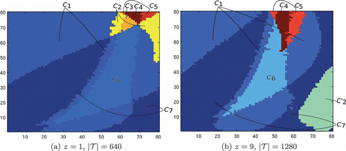
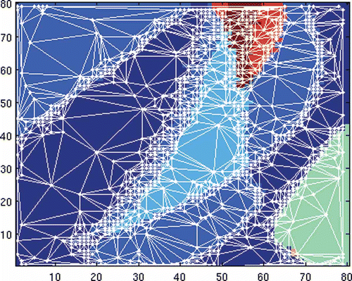
Figure 7 shows the Delaunay triangulation of the final training set over the classifications given by the 1-NN algorithm. This image illustrates the algorithm’s ability to enhance resolution around the boundaries of the equivalence classes in parameter space.

Figure 7. Delaunay triangulation of generated using AlgorithmD; z = 9, .

Table 1 shows the misclassification of the database by compiling all of the z slice calculation, along with a comparison to a training set generated uniformly at random. For brevity, we will not discuss the results of the indvidual slices, however, there are noticeable differences between slices. Due to these differences, we are currently investigating incorporating an adaptive budget to allocate the training set based on the complexity of the slices.

Table 1. Results for compilation of 2D z slices for AlgorithmD, AlgorithmN and Uniform Sampling.

Training set %	AlgorithmD	AlgorithmN	Uniform
10%	4.5	4.9	7.13
20%	1.1	2.78	4.98

6.1.2. ALGORITHMN

In this section, we review the results of AlgorithmN for the two-dimensional case. As expected, a slightly elevated misclassification rate is the price for increased computational efficiency. Figure 8 shows a plot of misclassification compared to a training set generated uniformly at random. In order to highlight the regions of the parameter space AlgorithmN focuses on, we plot the training set over a 1-NN classification below. The colour of the training set elements darken in proportion to the size of the current training set.

Figure 8. Plot of training set for AlgorithmN on z = 1, , misclassification of 123 grid elements, or 1.92% of ; the shade of a training set element depends upon when it was selected in the process of constructing . Classes correspond to those in Figures 5 and 6.

6.1.3. Slices in x and y directions

In order to further validate this algorithm, we ran both AlgorithmD and AlgorithmN on slices in the x and y direction as well. For brevity, we only show the results for 20% of the domain.

6.2. Three-dimensional domain

In Table 2, we display the results from AlgorithmN applied to the entire three-dimensional domain, instead of dividing the domain into slices. We only include results for AlgorithmN, as the overhead of constructing the Delaunay triangulation in three dimensions yields AlgorithmD unwieldy.

Table 2. Results for 3D Variants of AlgorithmN and Uniform Sampling.

Training set %	AlgorithmN	Uniform
10%	5.74	7.46
20%	3.19	5.86

7. Discussion

In this paper, we introduced an approach to predict bifurcations using machine learning incorporated into the Conley–Morse database framework. This approach to the study of complex dynamical systems provides a rich description of the system in both the phase space and the parameter space. This is especially relevant in biological sciences, where obtaining precise values of parameters often requires extensive collection of experimental data. For instance, certain models of chemotaxis [35] involve upwards of seventeen parameters, some only known approximately, and that range across eight orders of magnitude. In the database framework described in Section 2, the parameters vary over a range of values, with the rigorous results valid over that entire region in parameter space. Usually, a substantial effort must be spent validating and tuning model parameters [36]. The database framework shifts this emphasis to the analysis of the database results to find a range of parameters where model prediction is consistent with the data.

Even though computationally efficient, the database description of the parameter space still suffers from the curse of dimensionality. We have shown that active sampling techniques based on assumptions of the underlying dynamics in combination with a straightforward k-NN classifier can lead to very accurate predictions of regions around potential bifurcations, thereby alleviating some of the computational burden due to high-dimensional parameter spaces. In particular, one can approximate the Conley–Morse database with greater than 97% accuracy through computing only 20% of the total Morse graphs.

We are currently working to incorporate adaptive computation into the database construction in order to provide rigorous continuation classes at lower computational cost. Furthermore, we are also investigating additional nonlinear systems with higher-dimensional parameter spaces. The presentation and exposition of this paper has focused on dynamical systems in the form of discrete maps. However, similar theoretical ideas apply to dynamical systems represented by differential equations, and extending the Conley–Morse database to differential equations is currently being investigated. In contrast to maps, constructing the combinatorial representation requires rigorous numerical calculation, which incurs a much greater computational cost than evaluating a map. Therefore, a machine learning approach such as the one presented in this paper becomes even more relevant in such a setting.

Acknowledgements

KS was partially supported by DARPA grant D12AP200025, JB was partially supported by NSF DMS 0955604, and TG was partially supported by NSF grant DMS-1226213, DARPA D12AP200025 and NIH R01 grant 1R01AG040020-01.

References

- Y. Bar-Yam, Dynamics of Complex Systems, 1st ed., Westview Pr, Cambridge, MA, 1997.
- S.A. Levin, Complex adaptive systems: Exploring the known, the unknown and the unknowable. Bull. Am. Math. Soc. 40 (1) (2002), pp. 3–19.
- M. Costa, I. Ghiran, C.K. Peng, A. Nicholson-Weller, and A.L. Goldberger, Complex dynamics of human red blood cell ickering: Alterations with in vivo aging. Phys. Rev. E (2008), pp. 1–4.
- M.E.J. Newman, The structure and function of complex networks. SIAM Rev. 45 (2) (2003), pp. 167–256.
- C. Bianca, Onset of nonlinearity in thermostatted active particles models for complex systems. Nonlinear Anal. Real World Appl. 13 (6) (2012), pp. 2593–2608.
- S.M. Glaser, M.J. Fogarty, H. Liu, I. Altman, C.-H. Hsieh, L. Kaufman, A.D. MacCall, A.A. Rosenberg, H. Ye, and G. Sugihara, Complex dynamics may limit prediction in marine fisheries. Fish. Fish. ( 2013). Available at http://dx.doi.org/10.1111/faf.12037.
- G. Sugihara, Nonlinear forecasting as a way of distinguishing chaos from measurement error in time series. Nature 344 (1990), pp. 734–741.
- E.N. Lorenz, Irregularity: A fundamental property of the atmosphere. Tellus A 36A (2) (1984), pp. 98–110.
- T.M. Lenton, H. Held, E. Kriegler, J.W. Hall, W. Lucht, S. Rahmstorf, and H.J. Schellnhuber, Tipping elements in the Earth’s climate system. Proc. Natl. Acad. Sci. USA 105 (6) (2008), pp. 1786–1793.
- S. Rahmstorf, M. Crucifix, A. Ganopolski, H. Goosse, I. Kamenkovich, R. Knutti, G. Lohmann, R. Marsh, L.A. Mysak, Z. Wang, and A.J. Weaver, Thermohaline circulation hysteresis: A model intercomparison. Geophys. Res. Lett. 32 (23) (2005), pp. 1–5.
- M. Scheer, J. Bascompte, W.A. Brock, V. Brovkin, S.R. Carpenter, V. Dakos, H. Held, E.H. Van Nes, M. Rietkerk, and G. Sugihara, Early-warning signals for critical transitions. Nature 461 (7260) (2009), pp. 53–59.
- P.D. Ditlevsen and S.J. Johnsen, Tipping points: Early warning and wishful thinking. Geophys. Res. Lett. 37 (19) (2010), pp. 2–5.
- O.M. Johannessen, K. Khvorostovsky, M.W. Miles, and L.P. Bobylev, Recent ice-sheet growth in the interior of Greenland. Science (New York, N.Y.) 310 (5750) (2005), pp. 1013–1016.
- E. Rignot, I. Velicogna, M.R. van den Broeke, A. Monaghan, and J. Lenaerts, Acceleration of the contribution of the Greenland and Antarctic ice sheets to sea level rise. Geophys. Res. Lett. 38 (5) (2011), pp. 1–5.
- Z. Arai, W. Kalies, H. Kokubu, K. Mischaikow, H. Oka, and P. Pilarczyk, A database schema for the analysis of global dynamics of multiparameter systems. SIAM J. Appl. Dyn. Syst. 8 (3) (2009), p. 757.
- K. Mischaikow and M. Mrozek, Conley index theory, in Handbook of Dynamical Systems II: Towards Applications, B. Fiedler, ed., chapter 9, North-Holland, Amsterdam, 2002, pp. 393–460.
- K. Mischaikow, The Conley Index Theory: A Brief Introduction. Banach Center Publications, 47, 1999.
- J. Berwald, T. Gedeon, and J. Sheppard, Using machine learning to predict catastrophes in dynamical systems. J. Comput. Appl. Math. 236 (9) (2012), pp. 2235–2245.
- T. Kaczynski, K. Mischaikow, and M. Mrozek, Computational Homology. Springer, New York, 2004.
- M. Dellnitz, G. Froyland, and O. Junge, The algorithm behind GAIO – Set oriented numerical methods for dynamical systems, in Ergodic Theory, Analysis, and Efficient Simulation of Dynamical Systems, B. Fiedler, ed., Springer, New York, 2000, pp. 145–174.
- A. Katok and B. Hasselblatt, Introduction to the Modern Theory of Dynamical Systems, Cambridge University Press, Cambridge, UK, 1995.
- D. Ludwig, D.D. Jones, and C.S. Holling, Qualitative analysis of insect outbreak systems: The spruce budworm and forest. J. Animal Ecol. 47 (1) (1978), pp. 315–332.
- J.D. Murray, Mathematical Biology: I. An Introduction. Interdisciplinary Applied Mathematics. Springer, New York, 2002.
- W. Tucker, Validated Numerics, 1st ed., Princeton University Press, Princeton, NJ, 2011.
- I. Ugarcovici and H. Weiss, Chaotic dynamics of a nonlinear density dependent population model. Nonlinearity 17 (2004), pp. 1689–1711.
- B. Settles, Active learning literature survey, Computer Sciences Technical Report 1648, University of Wisconsin–Madison, Madison, WI, 2009.
- S. Tong and E. Chang, Support Vector Machine Active Learning for Image Retrieval, Proceedings of the Ninth ACM International Conference on Multimedia, MULTIMEDIA ‘01, New York, ACM, New York, 2001, pp. 107–118.
- E. Alpaydin, Introduction to Machine Learning, 2nd ed., MIT Press, Cambridge, MA, 2010.
- M. Hasenjger and H. Ritter, Active learning with local models. Neural Process. Lett. 7 (1998), pp. 107–117. doi:10.1023/A:1009688513124
- M. de Berg, O. Cheong, M. van Kreveld, and M. Overmars (eds.), Delaunay triangulations, in Computational Geometry: Algorithms and Applications, chapter 9. Springer Verlag, Berlin, 2008, pp. 191–218.
- U. Schöning, Graph isomorphism is in the low hierarchy. J. Comput. Syst. Sci. 37 (3) (1988), pp. 312–323.
- P. Indyk and R. Motwani, Approximate Nearest Neighbors: Towards Removing the Curse of Dimensionality. Proceedings of the Thirtieth Annual ACM Symposium on Theory of Computing, STOC ′98, New York, ACM, New York, 1998, pp. 604–613.
- N. Katayama and S. Satoh, The sr-tree: An index structure for high-dimensional nearest neighbor queries. SIGMOD Rec. 26 (2) (1997), pp. 369–380.
- P.N. Yianilos, Data Structures and Algorithms for Nearest Neighbor Search in General Metric Spaces. Proceedings of the Fourth Annual ACM-SIAM Symposium on Discrete Algorithms, SODA ‘93, Philadelphia, PA, Society for Industrial and Applied Mathematics, Philadelphia, PA, 1993, pp. 311–321.
- M.P. Neilson, D.M. Veltman, P.J.M. van Haastert, S.D. Webb, J.A. Mackenzie, and R.H. Insall, Chemotaxis: A feedback-based computational model robustly predicts multiple aspects of real cell behaviour. PLoS Biol. 9 (5) (2011), p. e1000618.
- C. Bianca, Thermostatted models multiscale analysis and tuning with real-world systems data. Phys. Life Rev. 9 (4) (2012), pp. 418–425.