Model order reduction for numerical simulation of particle transport based on numerical integration approaches

Abstract

In this article, we present a non-linear model order reduction (MOR) method based on a linearization technique for a model of particle transport. Historically, non-linear differential equations have been applied to model particle transport. Such non-linear differential equations are expensive and time-consuming to solve. This is a motivation for reducing such a model, based on molecular collisions for heavy particle transport in plasma reactors. Here, we reduce the order by linearization with numerical integration approaches and obtain a controllable and calculable transport–reaction model.

We linearize the transport model of the heavy particles with numerical fixed point schemes to a general linear control systems (GLCSs); see M.A. Lieberman and A.J. Lichtenberg [Principle of Plasma Discharges and Materials Processing, 2nd ed., Wiley-Interscience, 2005]. Such linearization allows modelling the collision of the plasma reactor by a system of ordinary differential equations; see the models in M. Ohring [Materials Science of Thin Films, 2nd ed., Academic Press, San Diego, CA, 2002]. Because of their non-linearity, we extend the linear splitting methods with linearization techniques to solve these non-linear equations. Numerical simulations are used to validate this modelling and linearization approach.

The contribution is to reuse linear reaction models without neglecting the delicate extension to non-linear reaction models. With the help of higher-order quadrature rules, e.g. Simpson’s rule, we obtain sufficient accuracy and replace the non-linear models by a simpler lower-order linear model.

Numerical simulations are presented to validate the coupling ideas of the linearized model.

Keywords:

• model order reduction
• numerical integration
• iterative splitting method
• linearization
• non-linear differential equations
• convection–diffusion–reaction equation
• model verification

AMS Subject Classification:

• 35J60
• 35J65
• 65M99
• 65N12
• 65Z05
• 74S10
• 76R50

1. Introduction

Non-linear processes are well known in many electrochemical applications and historically they have been modelled by non-linear systems of coupled partial and ordinary differential equations (ODEs) (see [1,2]).

We are motivated to understand the microscopic and macroscopic model influence on the transport behaviour of a plasma-enhanced chemical vapour deposition (PE-CVD) process to control an optimal transport process in the apparatus (see [3,4]).

In recent years, due to research in producing high-temperature films by deposition at low pressures, there have been an increasing number of such processes. To understand the deposition of a thin film by a CVD apparatus, a complete study of microscopic models with non-linear reactions is necessary (see [5]).

For solving such physical phenomena numerically, kinetic approaches based on Boltzmann equation [6,7] have been used significantly. Systems of coupled Boltzmann equations are difficult to solve analytically and for many years, both analytical and numerical methods have been continuously proposed (see [8,9]). We concentrate on particle methods, which are a class of numerical methods; for an overview (see [6,10]). To apply particle methods to the Boltzmann equation, one can use two main ideas in treating the collision integral:

• Stochastic or

• deterministic approach.

In the stochastic approach, the particle methods are based on the Monte Carlo (MC) method (see [11]), modelling the collision probabilities using stochastic events. New approaches to stochastic approaches are discussed in [12]. In the deterministic approach, the particle methods use particles as quadrature nodes for computing an approximate solution of the collision integral (see [13]). In such methods, the particles are kept fixed in the velocity space, and the evolution is reflected in changing their weights in time (see [14,15]).

Another framework of deterministic particle methods is given by a different approach, later called the MottaWick Flux (MWF) method (see [16]). Here, the idea is to rewrite the equation in divergence form and transform the problem into a collisionless equation. This is done by defining a flux equivalent to the inhomogeneity and by computing at each time step the collision-induced force term for the collisionless problem. Later, the formulation of the method for implementation purposes was discussed by [17] and [18]. A new formulation of the MWF method, which is generalized to the system of the Boltzmann equation, is done in [19]. They discuss the convergence analysis for the one-dimensional case, which is given in [20]. The comparison of the MWF method with other important particle methods was presented in the framework of [21].

In the present article, we also deal with the deterministic approach of particle methods. We present a model order reduction (MOR) method to replace the original non-linear microscopic system by an approximating system with much smaller state space dimensions (see also [22]. As a result, it can significantly reduce the design time and allow concentrating on more design strategies (see [23–25]). The basic idea is a linearization based on numerical integrators (see [26,27]) of such a microscopic process, so that we can model the transport processes in thin layers, e.g., the implantation or deposition of metallic or ceramic materials. Such improved material models allow studying thin layers more carefully and can be used in the production of the so-called metallic bipolar plates (see a reduced order model [28]). Our plasma, which is the transport medium in the CVD process, is modelled by a Boltzmann equation for the heavy particles. For their drift, we use a classical diffusion equation. We simplify by neglecting the electron modelling, because their influence is sufficiently small.

Numerical approximations are necessary to solve such non-linear models. In order to obtain efficient solvers and to ameliorate the burden of their coding, we contribute an iterative operator splitting method. First, we extend such a linear scheme to a time-dependent and a non-linear scheme based on the idea of linearizing the non-linear terms. For the spatial and time discretization, we apply standard finite difference methods of higher order. For the linearization techniques, we apply fixed point and higher-order quadrature rules to solve the non-linear scheme. Second, we rewrite the linearized and discretized scheme as a GLCS (see [29,30]). Such control systems are written as ODEs and are solved with splitting techniques.

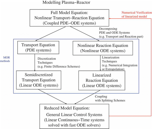
The idea of MOR methods, which are based on reducing the non-linear transport–reaction equation to compute a system of linearized ODEs, is presented in Figure 1.

Figure 1. Modelling plasma reactors with linearization and splitting techniques.

The outline of this article is as follows. In Section 2, we present our mathematical model and a possible reduced model for further approximations. Further on in Section 3, we discuss the discretization, transformation and linearization techniques to obtain a GLCS. The numerical simulations are given in Section 4. Section 5 summarizes our results.

2. Mathematical model for the plasma reactor

For many years now, plasma-enhanced chemical vapour deposition (PE-CVD) processes have been used to deposit thin films on metallic plates (see [3]). The growth of such a thin film by PE-CVD processes is modelled by [1,2]. The technical processes are very delicate, and real-life experiments are expensive (see [3]). One of the main problems is the large physical parameter space, while the number of possible experiments involves at least the variation of all possible parameters. Here, numerical simulations seem to be an alternative for reducing the large number of experiments required, and helping to derive a reduced parameter space based on mathematical modelling. An overview of the PE-CVD process is discussed in the following paragraphs.

The precursor gases (e.g. tetraethyltitanium) are transported and diffused to an electric field under very low-pressure conditions $(<\mathrm{T}\mathrm{o}\mathrm{r}\mathrm{r})$. We obtain at least a non-equilibrium plasma (see [31,32]), which can be modelled by a particle transport model (see [33]). This ionized background medium, also known as ‘cold’ plasma or glow discharges, helps to modify the surface of the thin film plates (see the applications in [34,32]).

PE-CVD processes are controllable methods to influence the chemical processes, by pressure, by temperature and by the precursor gases. The processes have been developed recently and are well-known design tools for producing high-temperature films (see [2]). We consider models that are related to upscaled microscopic scales and embedded into mesoscopic scales [8]. We assume that the thin layer material is a homogeneous medium and that the surface can be modelled as a porous medium [35]. Additional, physical experiments are done to measure the influence of the temperature, pressure and plasma power on the deposition rates (see [36] and [3]). They applied the plasma reactor chamber of an NIST GEC reference cell and used a hybrid inductively coupled plasma (ICP)/capacitively coupled plasma (CCP)-RF plasma source (see [36]).

In the following, the non-linear model of the plasma reactor is based on the ideas in [4,8,37]. An advantage of such a model is the decoupling into linear and non-linear processes of the model.

The full model is based on coupled convection–diffusion–reaction equations, while the convection–diffusion equations are linear partial differential equations (PDEs), and the reaction equations are non-linear ODEs.

The system of differential equations is given by

(1) $\frac{\mathrm{\partial }}{\mathrm{\partial }t}{c}_i+\mathrm{\nabla }{F}_i-R_{g,i}(c)=0\mathrm{i}\mathrm{n}\mathrm{\Omega }\times [0,t]$(1)

$F_i=v{c}_i-D\mathrm{\nabla }{c}_i+\eta E{c}_i$

(2) $c_i(x,t)=c_{i,0}(x)\mathrm{o}\mathrm{n}\mathrm{\Omega }$(2)

(3) $c_i(x,t)=c_{i,1}(x,t)\mathrm{o}\mathrm{n}\mathrm{\partial }\mathrm{\Omega }\times [0,t]$(3)

where $c=(c_1,\dots ,c_m{)}^t$ is the particle density vector with $c_i$ being the ith species, $i=1,\dots ,n$ and n the number of species. $F_i$ is the flux of species i. $v$ is the flux velocity through the chamber and porous substrate [35] (which conserves momentum). D is the diffusion matrix, and $R_{g,i}(c)$ are the non-linear reaction functions of species i. The initial value is $c_{i,0}$, and we assume Dirichlet boundary conditions with the function $c_{i,1}(x,t)$ sufficiently smooth. E is the electric field, and $\eta$ the mobility (see [38]).

While the linear processes are slow, the non-linear processes are fast, and we assume the following separation of the two parts:

• Transport part (linear) and

• Reaction part (non-linear).

In the following section, we discuss these two parts.

2.1. Transport part

The modelling of the transport part is based on the transport equation and the flow equation in the plasma reactor.

(4) $\frac{\mathrm{\partial }}{\mathrm{\partial }t}{c}_i+\mathrm{\nabla }{F}_i=0\mathrm{i}\mathrm{n}\mathrm{\Omega }\times [0,t]$(4)

$F_i=v{c}_i-D\mathrm{\nabla }{c}_i+\eta E{c}_i,$

(5) $c_i(x,t)=c_{i,0}(x)\mathrm{o}\mathrm{n}\mathrm{\Omega }$(5)

(6) $c_i(x,t)=c_{i,1}(x,t),\mathrm{o}\mathrm{n}\mathrm{\partial }\mathrm{\Omega }\times [0,t]$(6)

where the unknowns are given by $c_1=c_1(x,t)$ till $c_m=c_m(x,t)$ in $(0,T){\subset }^{+}$ with $i=1,\dots ,m$, and m is the number of species. We assume the same densities $c_0$ till $c_m$ of the species as initial condition. We assume Dirichlet boundary conditions (see [39]).

Furthermore, the computation of $v$ is based on the conservation of momentum and given as the flow field (Navier–Stokes equation):

(7) $\frac{\mathrm{\partial }}{\mathrm{\partial }t}v+v\cdot \mathrm{\nabla }v=-\mathrm{\nabla }p\mathrm{i}\mathrm{n}\mathrm{\Omega }\times [0,t]$(7)

(8) $v(x,t)=v_0(x)\mathrm{o}\mathrm{n}\mathrm{\Omega }$(8)

(9) $v(x,t)=v_1(x,t)\mathrm{o}\mathrm{n}\mathrm{\partial }\mathrm{\Omega }\times [0,t]$(9)

where $v$ is the velocity field, p is the pressure, $v_0$ is the initial condition of the velocity field, $v_1$ is the Dirichlet boundary condition of the velocity field and the position vector is $x={(x_1,x_2,x_3)}^t\in \Omega \subset {\text{I-1R}}^{3,+}$. Furthermore, we assume that the flow is divergence-free, and the pressure is predefined.

The electric field is given as a distribution related to the charge density, which can be computed by the Maxwell equations (see [40]). Furthermore, it is necessary to solve the Poisson equation which relates the divergence of the local electric fields to the charge density [38]:

(10) $\mathrm{\nabla }\cdot E=\frac{e}{{\text{egr}}_0}\sum _{i=1}^n{Z}_i{c}_i,$(10)

where e is an element charge, ${\text{egr}}_0$ is the permittivity of the gas mixture, $c_i$ is the particle density of species i and $Z_i$ is the relative charge of species i (see [4]).

Under the assumption of a near vacuum and a near equilibrium plasma, the charge densities can be approximated as constants (see [1,11]). We apply the assumptions in the following simplification of the upscaled electric field discussed in [37]:

(11) $\mathrm{\nabla }\cdot E\approx \frac{e}{{\text{egr}}_0}\sum _{i=1}^n{Z}_i{c}_{\mathrm{c}\mathrm{o}\mathrm{n}\mathrm{s}\mathrm{t},i}{|}_{{\mathrm{\Omega }}_j}$(11)

where we assume that $c_i\approx c_{\mathrm{c}\mathrm{o}\mathrm{n}\mathrm{s}\mathrm{t},i}\mathrm{f}\mathrm{o}\mathrm{r}{\mathrm{\Omega }}_j$ is a constant particle density of species i in the domain ${\mathrm{\Omega }}_j$, with $j\in 1,\dots ,m$, and m is the number of the domains in the electric field.

2.2. Reaction part

For the reaction part, we have given non-linear differential equations:

(12) $\frac{\mathrm{\partial }}{\mathrm{\partial }t}{c}_i-R_{g,i}(c)=0\mathrm{i}\mathrm{n}\mathrm{\Omega }\times [0,t]$(12)

(13) $c_i(x,t)=c_{i,0}(x)\mathrm{o}\mathrm{n}\mathrm{\Omega }$(13)

where the non-linear functions $R_{g,i}$ are given by

(14) $R_{g_i}={\lambda }_{1,i}{c}_1^{n_{i,1,1}}\dots c_m^{n_{i,1,m}}+\dots +{\lambda }_{m,i}{c}_1^{n_{i,m,1}}\dots c_m^{n_{i,m,m}}$(14)

where ${\lambda }_{1,1},\dots ,{\lambda }_{m,m}\in$ and the exponents $n_{1,1,1},\dots ,n_{m,m,m}\in$.

For simplification, we deal with the following reaction part:

(15) $R_{g_i}={\lambda }_{1,i}{c}_1^{n_i}+{\lambda }_{2,i}{c}_i$(15)

where ${\lambda }_1,{\lambda }_2{\in }^{+}$ and $n_i\in I{N}^{+,0}$.

3. Application of MOR methods

In the following, we apply MOR methods to approximate the original system of non-linear equations to a computable and linearized equation system.

MOR methods have been well known for many years and discussed in MOR technology, e.g. the fast simulation of non-linear circuits [23], the analysis of non-linear circuits [22], generating low-cost macromodels [25], etc.

We apply such ideas in the following manner to our model equations:

• Semi-discretization via finite difference or finite volume methods to transform it to a system of non-linear ODEs (see [41]).

• Linearization via numerical integration to transform it to a linear ODE based on a fixed point problem (see [22]).

• Analytical solutions via a GLCS for special time-dependent approaches (see [29])

• Decomposition via an iterative splitting scheme to transform it to simpler linear ODE s (see [42]).

We deal with the following non-linear PDE given in (1) and rewritten as an operator equation:

(16) $\frac{\mathrm{\partial }U}{\mathrm{\partial }t}+AU+B(U,t)$(16)

(17) $U(x,t)=U_0(x)\mathrm{o}\mathrm{n}\mathrm{\Omega }$(17)

(18) $U(x,t)=U_1(x,t)\mathrm{o}\mathrm{n}\mathrm{\partial }\mathrm{\Omega }\times [0,t]$(18)

where $U=(u_1,\dots ,u_m{)}^t$ is the solution vector with $c_i$ being the ith species, $i=1,\dots ,n$ and n the number of species.

The operators are given by

(19) $A=\left(\begin{array}{cccc}\mathrm{\nabla }\cdot v-\mathrm{\nabla }{D}_{11}\mathrm{\nabla }& -\mathrm{\nabla }{D}_{12}\mathrm{\nabla }& \dots & -\mathrm{\nabla }{D}_{1m}\mathrm{\nabla }\\ \mathrm{\nabla }\cdot v-\mathrm{\nabla }{D}_{21}\mathrm{\nabla }& -\mathrm{\nabla }{D}_{22}\mathrm{\nabla }& \dots & -\mathrm{\nabla }{D}_{2m}\mathrm{\nabla }\\ ⋮& ⋮& \ddots & ⋮\\ \mathrm{\nabla }\cdot v-\mathrm{\nabla }{D}_{m1}\mathrm{\nabla }& -\mathrm{\nabla }{D}_{m2}\mathrm{\nabla }& \dots & -\mathrm{\nabla }{D}_{mm}\mathrm{\nabla }\end{array}\right)$(19)

(20) $B(U,t)=\left(\begin{array}{c}{R}_{g,1}(U)\\ R_{g,2}(U)\\ ⋮\\ R_{g,m}(U)\end{array}\right)+\nu EU$(20)

where $v$ is the flux velocity, D is the diffusion matrix with the matrix entries $D_{ij}\in {\text{I-1R}}^{+},i,j=1,\dots ,m$ and $R_{g,i}(U)$ are the non-linear reaction functions of species $i=1,\dots ,m$.

3.1. Semi-discretization

In the first step, we transform the given PDE (16) into a system of ODE. Such systems can be considered as GLCSs and further approximated with MOR methods.

For the transformation to a system of ODEs, we have to apply the following numerical schemes to the PDE:

• Finite difference schemes (see [43]).

• Finite volume schemes (see [41]).

In the following, we concentrate on applying a higher-order finite difference scheme (see [43]):

$v_i\mathrm{\nabla }{u}_i\approx v_{i,x}\frac{-\frac{1}{2}{u}_i^{j+1,k,l}+2u_i^{j,k,l}-\frac{3}{2}{u}_i^{j-1,k,l}}{\mathrm{\Delta }\mathrm{x}}$

$+v_{i,y}\frac{-\frac{1}{2}{u}_i^{j,k+1,l}+2u_i^{j,k,l}-\frac{3}{2}{u}_i^{j,k-1,l}}{\mathrm{\Delta }\mathrm{y}}$

(21) $+v_{i,z}\frac{-\frac{1}{2}{u}_i^{j,k,l+1}+2u_i^{j,k,l}-\frac{3}{2}{u}_i^{j,k,l-1}}{\mathrm{\Delta }\mathrm{z}}$(21)

$\mathrm{\nabla }{D}_{i,\tilde{i}}\mathrm{\nabla }{u}_i\approx D_{i,\tilde{i},x}\frac{u_i^{j+1,k,l}-2u_i^{j,k,l}+u_i^{j-1,k,l}}{\mathrm{\Delta }{\mathrm{x}}^2}+D_{i,\tilde{i},y}\frac{u_i^{j,k+1,l}-2u_i^{j,k,l}+u_i^{j,k-1,l}}{\mathrm{\Delta }{\mathrm{y}}^2}$

(22) $+D_{i,\tilde{i},z}\frac{u_i^{j,k,l+1}-2u_i^{j,k,l}+u_i^{j,k,l-1}}{\mathrm{\Delta }{\mathrm{z}}^2},\tilde{i}\in 1,\dots ,m$(22)

where $j\in 1,\dots ,J,k\in 1,\dots ,K,l\in 1,\dots ,L$ are the spatially discretized points.

Then the PDEs (16) can be written as a system of ODEs:

(23) $U^{\prime }=\tilde{A}U+B(U,t)+F(t)$(23)

(24) $U(0)=U_0$(24)

where $U=(u_1,\dots ,u_m{)}^t$ and the discrete $u_i=(u_i^{1,1,1},\dots ,u_i^{J,K,L}{)}^t$. The boundary conditions are included in the right-hand side $F(t)$. Furthermore, the linear operator $\tilde{A}$ is the approximated transport part, and the non-linear operator $\tilde{B}(U)$ is the non-linear reaction part.

3.2. Linear model order reduction techniques

In the following, we discuss the MOR methods based on linearization, numerical integration and analytical approaches.

The treatment for the operator $B(U,t)$, which is a non-linear bounded operator on an appropriate Banach space to get a reduced model, is discussed as follows:

• Classical piecewise-linear schemes (linearization approach),

• Fixed point schemes (numerical integration approach),

• Analytical solutions of simpler non-linear equations (analytical approach) and

• Analytical approach via GLCS (control approach).

Remark 1. For the linearized schemes, we assume that the linear eigenvalue space of the solutions is embedded into the non-linear eigenvalue space. Furthermore, we assume that a solution of the derived fixed point schemes exists (see [44]).

Classical piecewise-linear schemes

For the piecewise-linear schemes, we apply the general non-linear scheme and obtain a set of s linearized states $U_0,U_1,\dots ,U_s$ generated by the linear system of

(25) $U_{i+1}^{\prime }=B(U_i,t)+J_i(U_{i+1}-U_i)$(25)

where $J_i=\frac{\mathrm{\partial }B(U_i,t)}{\mathrm{\partial }U}$ is the Jacobian of $B(U,t)$ evaluated at $U_i$.

Here, we have a quadratic approach to the non-linear scheme; for the proofs, see [29].

Numerical integration approach

The numerical integration approach deals with the idea by linearizing the non-linear model by solving the integral formulation (see [45]). The integral formulation of the non-linear reaction equations of our model (12) can be written as the following non-linear system of ODEs:

${\int }_0^t{U}^{\prime }\mathrm{d}t={\int }_0^{t}B(U,t)\mathrm{d}t$

(26) $U(t)-U(0)={\int }_0^{t}B(U,t)\mathrm{d}t\approx t{B}_{\mathrm{a}\mathrm{p}\mathrm{p}\mathrm{r}\mathrm{o}\mathrm{a}\mathrm{c}\mathrm{h}}(U(0),U(t),t)\mathrm{w}\mathrm{i}\mathrm{t}\mathrm{h}U\ne 0$(26)

where $B(U,t)=\tilde{B}(U,t)U$. Furthermore, with the numerical integration approach, we have $B_{\mathrm{a}\mathrm{p}\mathrm{p}\mathrm{r}\mathrm{o}\mathrm{a}\mathrm{c}\mathrm{h}}(U(0),U(t),t)=B_{\mathrm{a}\mathrm{p}\mathrm{p}\mathrm{r}\mathrm{o}\mathrm{a}\mathrm{c}\mathrm{h}}(U(t),t)$. We can assume that the non-linear system $B(U(0))=0$ can be interpreted as the steady state of the non-linear ODE (38).

The non-linear problem can be reformulated as a fixed point problem:

(27) $U=K(U,t)\mathrm{w}\mathrm{i}\mathrm{t}\mathrm{h}U\ne 0$(27)

where $K(U,t)=U(0)+{\int }_0^{t}B(U,t)\mathrm{d}t$.

We have linear convergence in the fixed point scheme:

(28) $U_{i+1}=K(U_i)$(28)

where $i=1,\dots ,I$.

Theorem 1. Assume that $\Omega \subset \text{I-1R}$, and that $\text{K}:\Omega \to \text{I-1R}$ is a contraction mapping on $\mathrm{\Omega }$ with Lipschitz constant $\gamma <1$ with $\mathrm{K}(\mathrm{U})\in \mathrm{\Omega }$ for all $\mathrm{U}\in \mathrm{\Omega }$. Then there exists a unique fixed point of K (${\mathrm{U}}^{\ast }\in \mathrm{\Omega }$) and the fixed point scheme 29 converges linearly to ${\mathrm{U}}^{\ast }$.

The proof is discussed in [44].

Furthermore, for all $U_1,U_2$, and if $tM\le 1$ and if we assume $B_{\mathrm{a}\mathrm{p}\mathrm{p}\mathrm{r}\mathrm{o}\mathrm{a}\mathrm{c}\mathrm{h}}$ is bounded and Lipschitz continuous, so that we have $B_{\mathrm{a}\mathrm{p}\mathrm{p}\mathrm{r}\mathrm{o}\mathrm{a}\mathrm{c}\mathrm{h}}(U)\le M$, then the error of the fixed point scheme is linear.

(29) $||K(U_1)-K(U_2)||\le t|B_{\mathrm{a}\mathrm{p}\mathrm{p}\mathrm{r}\mathrm{o}\mathrm{a}\mathrm{c}\mathrm{h}}(U_1)-B_{\mathrm{a}\mathrm{p}\mathrm{p}\mathrm{r}\mathrm{o}\mathrm{a}\mathrm{c}\mathrm{h}}(U_2)|\le tM|U_1-U_2|$(29)

For general linearization ideas, we extend the fixed point schemes (see [44]), and we apply them to the following examples (see Example 1).

Example 1. In the following, we present some linearization techniques that we will apply in the numerical simulations:

• Time linearization

(30) ${\int }_0^{t}B(U,t)\mathrm{d}t=t{B}_{\mathrm{a}\mathrm{p}\mathrm{p}\mathrm{r}\mathrm{o}\mathrm{a}\mathrm{c}\mathrm{h}}(U,t)=t\tilde{B}(U(t^n))U(t)+O(t^2)$(30)

where we have a linear scheme with linear errors.

• Fixed point linearization

(31) ${\int }_0^{t}B(U,t)\mathrm{d}t=t{B}_{\mathrm{a}\mathrm{p}\mathrm{p}\mathrm{r}\mathrm{o}\mathrm{a}\mathrm{c}\mathrm{h}}(U,t)=t\tilde{B}(U_{i-1}(t))U_i(t)+O(t^2)$(31)

where we have a linear scheme with linear errors.

• Mixed linearizations (time and fixed point linearizations):

• Trapezoidal rule (linear approach)

(32) ${\int }_0^{t}B(U,t)\mathrm{d}t=t{B}_{\mathrm{a}\mathrm{p}\mathrm{p}\mathrm{r}\mathrm{o}\mathrm{a}\mathrm{c}\mathrm{h}}(U,t)=t\frac{\tilde{B}(U(t^n))+\tilde{B}(U_{i-1}(t))}{2}{U}_i(t)+O(t^3)$(32)

where we have a quadratic scheme with quadratic errors.

• Simpson’s rule (linear approach)

(33) $\begin{array}{rl}{\int }_0^{t}B(U,t)\mathrm{d}t& =t{B}_{\mathrm{a}\mathrm{p}\mathrm{p}\mathrm{r}\mathrm{o}\mathrm{a}\mathrm{c}\mathrm{h}}(U,t)\\ & =t\frac{\tilde{B}(U(t^n))+4\tilde{B}(U_{i-1}(t^{n+1/2}))+\tilde{B}(U_{i-1}(t^{n+1}))}{6}{U}_i(t)+O(t^5)\end{array}$(33)

where we have a fourth-order scheme with fourth-order errors.

• Richardson extrapolation (linear approach)

(34) ${\int }_0^{t}B(U,t)\mathrm{d}t=t{B}_{\mathrm{a}\mathrm{p}\mathrm{p}\mathrm{r}\mathrm{o}\mathrm{a}\mathrm{c}\mathrm{h}}(U,t)=t\frac{4\tilde{B}(U_{i-1}(t^{n+1/2}))-\tilde{B}(U_{i-1}(t^{n+1}))}{3}{U}_i(t)+O(t^4)$(34)

where we have a third-order scheme with third-order errors.

For the time discretization, we have $t\in [t^n,t^{n+1}]$ and $\mathrm{\Delta }t=t^{n+1}-t^n$ is the time-step with $n=1,\dots ,N-1$ being the discrete time-points.

Analytical Approach

In the following, we assume that we have special non-linear reaction equations of our model (12) that can be written as the following scalar Bernoulli differential equations:

(35) $u_i^{\prime }={\lambda }_{i,1}{u}_i+{\lambda }_{i,2}{u}_i^{\alpha }\mathrm{w}\mathrm{i}\mathrm{t}\mathrm{h}\mathrm{y}\ne 0\mathrm{a}\mathrm{n}\mathrm{d}\alpha \in I{N}^{+},\alpha >1$(35)

where $i=1,\dots ,m$, and m is the number of equations.

Such equations can be solved analytically; see [46].

We can transform each equation, using the substitution $w_i=\frac{1}{u_i^{\alpha -1}}$, and get

$\frac{u_i^{\prime }}{u_i^{\alpha }}+\frac{-{\lambda }_{i,1}}{u_i^{\alpha -1}}={\lambda }_{i,2}\Rightarrow \frac{w_i^{\prime }}{1-\alpha }+(-{\lambda }_{i,1})w_i={\lambda }_{2,i}.$

Now we multiply the equation by $M_i=exp((1-\alpha )\int -{\lambda }_{1,i}\mathrm{d}x)=exp(-(1-\alpha ){\lambda }_{1,i}x)$, integrate and resubstitute:

$\int (\frac{w_i^{\prime }}{1-\alpha }exp(-(1-\alpha ){\lambda }_{i,1}x)+(-{\lambda }_{i,1})w_{i}exp(-(1-\alpha ){\lambda }_{i,1}x))\mathrm{d}x$

$=\int ({\lambda }_{i,2}exp(-(1-\alpha ){\lambda }_{i,1}x))\mathrm{d}x$

$\frac{w_i}{1-\alpha }exp(-(1-\alpha ){\lambda }_{1}x)=-\frac{{\lambda }_{i,2}}{{\lambda }_{i,1}(1-\alpha )}exp(-(1-\alpha ){\lambda }_{i,1}x)+C_i,C_i\in \mathbf{R}$

$w_{i}exp(-(1-\alpha ){\lambda }_{i,1}x)=-\frac{{\lambda }_{i,2}}{{\lambda }_{i,1}}exp(-(1-\alpha ){\lambda }_{i,1}x)+C_i(1-\alpha )$

$\frac{1}{u_i^{\alpha -1}}exp(-(1-\alpha ){\lambda }_{i,1}x)=-\frac{{\lambda }_{i,2}}{{\lambda }_{i,1}}exp(-(1-\alpha ){\lambda }_{i,1}x)+C_i(1-\alpha ).$

After a transformation, we get the final solution of the differential equation as:

(36) $u_i=\sqrt[\alpha -1]{\frac{exp((\alpha -1){\lambda }_{i,1}x)}{-\frac{{\lambda }_{i,2}}{{\lambda }_{i,1}}exp((\alpha -1){\lambda }_{i,1}x)+C_i(1-\alpha )}}$(36)

for all $i=1,\dots ,m$.

Control approach (GLCS)

Based on the classical piecewise-linear schemes, see Equation (37), we can reformulate the problem into a well-known and analytically solvable GLCS (see [29]).

First, we assume the non-linear term is regularized to $B(U,t)\approx \tilde{B}(t)U$, and $\tilde{B}$ is a bounded time-dependent operator in an appropriate Banach space (see [30,47]).

Second, we rewrite the MOR model equation (37) to a set of s linearized states $U_0,U_1,\dots ,U_s$ by the linear system:

(37) $U_{i+1}^{\prime }=J_i(t)U_{i+1}+\hat{B}(t)v$(37)

where $J_i$ is the Jacobian of $B(U,t)$ and given in (37), the control operator is $\hat{B}(t)=\tilde{B}(t)-J_i$ and the system input is $v=U_i$.

Third, we can now apply the GLCS, using the following notations: $u=U_{i+1},v=U_i$, $A_1(t)=J_i(t)$, $A_2(t)=\tilde{B}(t)$.

The GLCS is then

(38) $\frac{\mathrm{d}u}{\mathrm{d}t}=A_1(t)u+A_2(t)v$(38)

(39) $\tilde{u}=C(t)u+D(t)v$(39)

(40) $u(0)=u_0$(40)

where the time-dependent operators are $A(t)\in X^n\times X^n$, $B(t)\in X^n\times X^m$, $C(t)\in X^p\times X^n$ and $D(t)\in X^p\times X^m$; $v:X\to X^m$ denotes the system input, $\tilde{u}:X\to X^p$ is the system output and $u:X\to X^n$ denotes the state vector. Furthermore, $X$ is an appropriate Banach space, e.g. U, a space of continuous or piecewise continuous functions.

The analytical solution of (38) and (39) is

(41) $u(t)=exp({\int }_0^t{A}_1(s)\mathrm{d}s{u}_0+{\int }_0^{t}exp({\int }_s^t{A}_1(\tilde{s})\mathrm{d}\tilde{s}{A}_2(s)v(s)\mathrm{d}s$(41)

(42) $\tilde{u}(t)=C(t)exp({\int }_0^t{A}_1(s)\mathrm{d}s{u}_0$(42)

$+C(t){\int }_0^{t}exp({\int }_s^t{A}_1(\tilde{s})\mathrm{d}\tilde{s}{A}_2(s)v(s)\mathrm{d}s+D(t)v(t)$

where we apply the fast computation of the exponential integral matrices via the Magnus expansion, see [47–49], and discuss in the following section.

Analytical approaches to time-dependent exponential matrices

In the analytical approach, the computation of the integrals in (41) and (42), where the operators are given as time-dependent exponential matrices, can be efficiently done by Magnus integrators (see [48] and [50]).

The Magnus integrator was introduced as a tool for solving time-dependent systems of differential equations (see [47]).

We treat the time-dependent differential equations

(43) $\frac{\mathrm{d}c}{\mathrm{d}t}=A(t)c(t)$(43)

where $c\in X(0,T{)}^m$ is a product space of dimension m, and $A(t)\in X(0,T{)}^m\times X(0,T{)}^m$ is a linear and bounded operator in the product space. $X$ is an appropriate Banach space with vector and operator norms.

The solution of (43) is

(44) $c(t)=exp({\int }_0^{t}A(s)\mathrm{d}s)c(0)=exp(\mathrm{\Omega }(t))c(0)$(44)

and the Magnus expansion is

(45) $\mathrm{\Omega }(t)=\sum _{n=1}^{\mathrm{\infty }}{\mathrm{\Omega }}_n(t)$(45)

where the first few terms are

${\mathrm{\Omega }}_1(t)={\int }_0^t\mathrm{d}{t}_1{A}_1$

(46) ${\mathrm{\Omega }}_2(t)=\frac{1}{2}{\int }_0^t\mathrm{d}{t}_1{\int }_0^{t_1}\mathrm{d}{t}_2[A_1,A_2]$(46)

where $A_n=A(t_n)$. We define the nth order Magnus operator to be the

(47) ${\mathrm{\Omega }}^{[n]}(t)=\mathrm{\Omega }(t)+O(t^{n+1})$(47)

such that

(48) $c(t)=exp[{\mathrm{\Omega }}^{[n]}(t)]c(0)+O(t^{n+1})$(48)

Remark 2. Explicitly, the second-order Magnus operator is

(49) $\begin{array}{rl}& {\mathrm{\Omega }}^{[2]}(t)={\int }_0^t\mathrm{d}{t}_{1}A(t_1)\\ & =tA\left(\frac{1}{2}t\right)+O(t^3)\end{array}$(49)

and the fourth-order Magnus operator is

(50) ${\mathrm{\Omega }}^{[4]}(t)=\frac{1}{2}t(A_1+A_2)-c_3{t}^2[A_1,A_2]$(50)

where $A_1=A(c_{1}t)$, $A_2=A(c_{2}t)$ and

(51) $c_1=\frac{1}{2}-\frac{\sqrt{3}}{6},c_2=\frac{1}{2}+\frac{\sqrt{3}}{6},c_3=\frac{\sqrt{3}}{12}$(51)

Remark 3. If we can linearize the problem (1) to a time-dependent problem and rewrite the problem to a GLCS, then the fast computation via exponential matrices is important (see [50]).

In the following, we concentrate on such non-linear approaches that are more efficient to solve via numerical integral linearization techniques.

4. Simulations for the plasma reactor

For the underlying plasma reactor model, first verification with real-life experiments was done in the work of [3]. Here, we compare the qualitative deposition results with the numerical simulations.

In the following numerical simulations, we concentrate on the numerical approaches of such experimentally verified models.

We introduce step by step the model equations for the plasma reactor and their improvements with MOR methods.

First, we present benchmark examples of non-linear differential equations based on the Bernoulli equations, which cover the reaction processes of the underlying species (see [5]). For the real-life application, we have derived such kinetic process in the reactor (see [26]).

Second, we present the numerical simulations of a realistic collision process in a plasma reaction and, finally, we discuss a TiC deposition process, which covers the transport and reaction parts of the model equations (see also [39]).

4.1. Test example: Bernoulli’s equation

In a first test example, we deal with the Bernoulli equation and explain the splitting ideas. Such reaction parts are often necessary to model complicated precursor gas reactions (see [39]).

Our equation is

(52) $\frac{\mathrm{d}y}{\mathrm{d}x}={\lambda }_{1}y+{\lambda }_2{y}^{\alpha },y(0)=1$(52)

where the non-linearity parameter is given by $\alpha \in I{N}^{+}$ and $\alpha >1$.

We have an analytical solution for $\alpha =3$; see Section 3.2 and [51]:

(53) $y=\sqrt{\frac{exp(-2t)}{-exp(-2t)+2}}$(53)

where we assume ${\lambda }_1=-1,{\lambda }_2=-1$.

Here, we decouple the linear and non-linear terms. We choose the time interval [0,1].

The operators for our splitting methods are

$Au={\lambda }_{1}u\mathrm{a}\mathrm{n}\mathrm{d}B(u)={\lambda }_2{u}^2(t^n)u$

where we linearize the term $B(u)={\lambda }_2{u}^2(t^n)u$.

The approximation error is calculated by the maximum error and is

$\mathrm{M}\mathrm{a}\mathrm{x}-\mathrm{e}\mathrm{r}\mathrm{r}\mathrm{o}\mathrm{r}={max}_{i,j}||u_{\mathrm{e}\mathrm{x}\mathrm{a}\mathrm{c}\mathrm{t}}(T)-u_{\mathrm{a}\mathrm{p}\mathrm{p}\mathrm{r}\mathrm{o}\mathrm{x}}(T)||.$

We test the following algorithms of the linearization techniques; see also Section 3.1.

Algorithm 41: Algorithms of Linearizations

We have implemented different linearization techniques to accelerate the solving process.

For all methods, we have $\mathrm{t}\in ({\mathrm{t}}^{\mathrm{n}},{\mathrm{t}}^{\mathrm{n}+1})$ with ${\mathrm{t}}^{\mathrm{n}+1}={\mathrm{t}}^{\mathrm{n}+\mathrm{k}\times \mathrm{h}}$, where h is the length of a time-step per interval and k is the number of time-steps per interval.

Here we use $\mathrm{k}=1000,100,10$ as the number of time-steps per interval.

1) time linearization

${\mathrm{u}}_{\mathrm{i}}^{\mathrm{m}}({\mathrm{t}}^{\mathrm{n}+\mathrm{h}\times (\mathrm{j}+1)})\approx {\mathrm{u}}_{\mathrm{i}}^{\mathrm{m}-1}(t^{n+h\cdot j})\times \mathrm{u}\text{nobreak}\mathrm{a}\mathrm{n}\mathrm{d}\mathrm{j}=0,1,\dots ,\mathrm{k}-1$

2) Fixed point linearization

${\mathrm{u}}_{\mathrm{i}}^{\mathrm{m}}({\mathrm{t}}^{\mathrm{n}+\mathrm{h}\times (\mathrm{j}+1)})\approx {\mathrm{u}}_{\mathrm{i}-1}^{\mathrm{m}-1}{(\mathrm{t}}^{\mathrm{n}+\mathrm{h}\times \mathrm{j}})\times \mathrm{u}\mathrm{a}\mathrm{n}\mathrm{d}\mathrm{j}=0,1,\dots ,\mathrm{k}-1$

3) Fixed point linearization

${\mathrm{u}}_{\mathrm{i}}^{\mathrm{m}}{(\mathrm{t}}^{\mathrm{n}+\mathrm{h}\times (\mathrm{j}+1)}{)\gg \mathrm{u}}_{\mathrm{i}-1}^{\mathrm{m}-1}{(\mathrm{t}}^{\mathrm{n}+\mathrm{h}\times (\mathrm{j}+1)})\times \mathrm{u}\mathrm{a}\mathrm{n}\mathrm{d}\mathrm{j}=0,1,\dots ,\mathrm{k}-1$

4) Trapezoidal linearization

${\mathrm{u}}_{\mathrm{i}}^{\mathrm{m}}{(\mathrm{t}}^{\mathrm{n}+\mathrm{h}\times (\mathrm{j}+1)})\gg \frac{{\mathrm{u}}_{\mathrm{i}}^{\mathrm{m}-1}{(\mathrm{t}}^{\mathrm{n}+\mathrm{h}\times \mathrm{j}}{)+\mathrm{u}}_{\mathrm{i}-1}^{\mathrm{m}-1}{(\mathrm{t}}^{\mathrm{n}+\mathrm{h}\times (\mathrm{j}+1)})}{2}\times \mathrm{u}\mathrm{a}\mathrm{n}\mathrm{d}\mathrm{j}=0,1,\dots ,\mathrm{k}-1$

5) Linearization with extrapolation methods, e.g., mixed fixed point linearization and time linearization: Simpson’s Rule

${\mathrm{u}}_{\mathrm{i}}^{\mathrm{m}}{(\mathrm{t}}^{\mathrm{n}+\mathrm{h}\times (\mathrm{j}+1)})\gg \frac{{\mathrm{u}}_{\mathrm{i}}^{\mathrm{m}-1}{(\mathrm{t}}^{\mathrm{n}+\mathrm{h}\times (\mathrm{j}-1)}{)+4\times \mathrm{u}}_{\mathrm{i}}^{\mathrm{m}-1}{(\mathrm{t}}^{\mathrm{n}+\mathrm{h}\times \mathrm{j}}{)+\mathrm{u}}_{\mathrm{i}-1}^{\mathrm{m}-1}{(\mathrm{t}}^{\mathrm{n}+\mathrm{h}\times (\mathrm{j}+1)})}{6}\times \mathrm{u}$

and j = 1, 2, …, k − 1

Remark: For $\mathrm{j}=0$ we use 4).

6) Same formula as 4) but with 1, 5, 50 intervals so that we can compare it directly with 5).

7) Linearization with extrapolation methods, e.g., mixed fixed point linearization and time linearization: Romberg’s method of order 5

${\mathrm{u}}_{\mathrm{i}}^{\mathrm{m}}{(\mathrm{t}}^{\mathrm{n}+\mathrm{h}\times (\mathrm{j}+1)})\gg \frac{{7\times \mathrm{u}}_{\mathrm{i}}^{\mathrm{m}-1}{(\mathrm{t}}^{\mathrm{n}+\mathrm{h}\times (\mathrm{j}-3)}{)+32\times \mathrm{u}}_{\mathrm{i}}^{\mathrm{m}-1}{(\mathrm{t}}^{\mathrm{n}+\mathrm{h}\times (\mathrm{j}-2)})}{90}$

$+\frac{{12\times \mathrm{u}}_{\mathrm{i}}^{\mathrm{m}-1}{(\mathrm{t}}^{\mathrm{n}+\mathrm{h}\times (\mathrm{j}-1)}{)+32\times \mathrm{u}}_{\mathrm{i}}^{\mathrm{m}-1}{(\mathrm{t}}^{\mathrm{n}+\mathrm{h}\times \mathrm{j}}{)+7\times \mathrm{u}}_{\mathrm{i}-1}^{\mathrm{m}-1}{(\mathrm{t}}^{\mathrm{n}+\mathrm{h}\times (\mathrm{j}+1)})}{90}\times \mathrm{u}and\mathrm{j}=3,4,\dots ,\mathrm{k}-1.$

Remark: In the following computations, we apply $j=0,1,2$ for the trapezoidal linearization. (see Algorithm 41, method 4))

In Table 1, we have compared the first four linearization methods (see Algorithm 41) for the non-linear equation (52) with $\alpha =3$. We present the absolute error with respect to the exact solution at the time point $t=1$.

Table 1. Numerical errors of the linearization techniques 1)–4) for the non-linearity $\alpha =3$.

$n_{\mathrm{i}\mathrm{t}}$	$n_{\mathrm{i}\mathrm{n}\mathrm{t}}$	$n_{\mathrm{t}\mathrm{s}}$	1)	2)	3)	4)
1	1	1000	9.8475e-2	9.8475e-2	9.8475e-2	9.8475e-2
1	10	100	9.8475e-2	9.8475e-2	9.8475e-2	9.8475e-2
1	100	10	9.8475e-2	9.8475e-2	9.8475e-2	9.8475e-2
2	1	1000	9.0918e-2	1.5120e-1	1.5081e-1	1.1983e-1
2	10	100	3.5313e-3	6.5402e-3	6.4061e-3	4.9586e-3
2	100	10	4.0558e-4	6.5628e-4	5.3055e-4	4.6807e-4
3	1	1000	1.2493e-2	6.5628e-4	2.2099e-2	1.7378e-2
3	10	100	1.5572e-4	3.4215e-4	3.3263e-4	2.4289e-4
3	100	10	1.8933e-6	3.3227e-6	2.4834e-6	2.1881e-6
4	1	1000	6.2378e-3	1.7962e-2	1.7332e-2	1.0961e-2
4	10	100	9.9185e-5	1.2001e-4	7.9856e-5	1.0473e-5
4	100	10	9.0573e-5	9.0986e-5	9.0857e-5	1.1228e-7
5	1	1000	6.3537e-4	2.0411e-3	1.8416e-3	1.1300e-3
5	10	100	7.1710e-6	8.1401e-6	6.8926e-6	2.2160e-7
5	100	10	4.9658e-7	4.9905e-7	8.3813e-7	1.6957e-7
6	1	1000	4.1674e-4	1.3140e-3	5.6985e-4	4.5031e-4
6	10	100	9.5261e-5	1.0045e-4	1.0032e-4	1.0809e-7
6	100	10	9.0569e-5	9.0972e-5	9.0879e-5	1.0153e-7

Notes: $n_{\mathrm{i}\mathrm{t}}$ – Number of iterations.

$n_{\mathrm{i}\mathrm{n}\mathrm{t}}$ – Number of intervals.

$n_{\mathrm{t}\mathrm{s}}$ – Number of time-steps per interval.

In Table 2, we have compared the last three linearization methods (see Algorithm 41) for the non-linear equation (52) with $\alpha =3$. We present the absolute error with respect to the exact solution at the time point $t=1$.

Table 2. Numerical errors of the linearization techniques 5)–7) for the non-linearity $\alpha =3$.

$n_{\mathrm{i}\mathrm{t}}$	$n_{\mathrm{i}\mathrm{n}\mathrm{t}}$	$n_{\mathrm{t}\mathrm{s}}$	5)	6)	7)
1	1	1000	9.8475e-2	9.8475e-2	9.8475e-2
1	10 (520)	100	9.8475e-2	9.8475e-2	9.8475e-2
1	100 (506)	10	9.8475e-2	9.8475e-2	9.8475e-2
2	1	1000	1.0035e-1	1.1983e-1	9.5693e-2
2	10 (520)	100	4.0352e-3	4.9725e-3	3.9457e-3
2	100 (506)	10	4.4931e-4	4.8199e-4	5.4264e-4
3	1	1000	1.4154e-2	1.7378e-2	1.3401e-2
3	10 (520)	100	1.8682e-4	2.4377e-4	1.8378e-4
3	100 (506)	10	2.1183e-6	1.8343e-6	2.5603e-6
4	1	1000	7.7274e-3	1.0961e-2	7.3968e-3
4	10 (520)	100	1.0074e-4	1.0918e-5	2.8216e-4
4	100 (506)	10	8.1542e-5	4.1890e-7	1.8985e-4
5	1	1000	8.0592e-4	1.1300e-3	8.7664e-4
5	10 (520)	100	7.1293e-6	2.9535e-7	2.0267e-5
5	100 (506)	10	3.6889e-7	6.7839e-7	8.0301e-7
6	1	1000	5.0661e-4	4.5031e-4	9.5049e-4
6	10 (520)	100	9.5053e-5	3.9646e-7	2.7745e-4
6	100 (506)	10	8.1536e-5	4.0604e-7	1.8985e-4

Notes: $n_{\mathrm{i}\mathrm{t}}$ – Number of iterations.

$n_{\mathrm{i}\mathrm{n}\mathrm{t}}$ – Number of intervals (in brackets for 6).

$n_{\mathrm{t}\mathrm{s}}$ – Number of time-steps per interval.

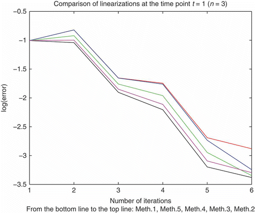
In the following, we compare graphically the linearization schemes in Figure 2 and obtain an overview of the best techniques.

Figure 2. The numerical errors of the different linearization techniques.

Remark 4. The best numerical and modelling preserving results were obtained by applying the trapezoidal rule for the linearization. Here, the number of iteration steps and the number of time partitions are balanced, so that neither more iteration steps nor a higher linearization scheme will be more efficient; see also [52]. Such a linearization technique has an optimal accuracy with respect to the full non-linear model and reduces the computational time of the modified model.

4.2. Test example: general Bernoulli’s equation

In more non-linear test examples, we deal with the Bernoulli’s equation, apply $\alpha =9$, and explain the splitting and linearization ideas.

Our equation is

(54) $\frac{\mathrm{d}y}{\mathrm{d}x}+p(x)y=q(x)y^{\alpha }\mathrm{w}\mathrm{i}\mathrm{t}\mathrm{h}y(0)\ne 0,\alpha \in I{N}^{+},\alpha >1$(54)

We concentrate on

(55) $y^{\prime }={\lambda }_{1}y+{\lambda }_2{y}^{\alpha }\mathrm{w}\mathrm{i}\mathrm{t}\mathrm{h}y(0)=1,$(55)

where $\alpha =9$. We have the analytical solution; see Section 3.2 and [51]:

(56) $y=\sqrt[8]{\frac{exp(-8x)}{-exp(-8x)+2}}.$(56)

Here, we decouple the linear and non-linear terms. We choose the time interval [0,1].

The operators for our splitting methods are

$Au={\lambda }_{1}u\text{and}Bu={\lambda }_2{y}^{\alpha },\text{and}\text{we}\text{choose}{\lambda }_1=-1,{\lambda }_2=-1.$

The approximation error is computed by the maximum error and given by

$1pt\text{Max}-\text{error}1pt={\text{max}}_{i,j}\left|\right|u_{\text{exact}}(T)-u_{\text{approx}}(T)\left|\right|.$

In Table 3, we have compared the first four linearization methods (see Algorithm 41) for the non-linear equation (53) with $\alpha =9$. We present the absolute error with respect to the exact solution at the time point $t=1$.

Table 3. Numerical errors of the linearization techniques 1)–4) for the non-linearity $\alpha =9$.

$n_{\mathrm{i}\mathrm{t}}$	$n_{\mathrm{i}\mathrm{n}\mathrm{t}}$	$n_{\mathrm{t}\mathrm{s}}$	1)	2)	3)	4)
1	1	1000	3.0525e-2	3.0525e-2	3.0525e-2	3.0525e-2
1	10	100	3.0525e-2	3.0525e-2	3.0525e-2	3.0525e-2
1	100	10	3.0525e-2	3.0525e-2	3.0525e-2	3.0525e-2
2	1	1000	4.2549e-2	7.3916e-2	7.3137e-2	5.6628e-2
2	10	100	1.5040e-3	5.8300e-3	5.6046e-3	3.4490e-3
2	100	10	2.2588e-4	5.3110e-4	3.5869e-4	2.9221e-4
3	1	1000	1.3013e-3	4.3157e-3	4.2140e-3	2.7381e-3
3	10	100	1.5103e-4	7.5462e-4	7.1752e-4	4.2603e-4
3	100	10	3.2169e-6	8.3987e-6	5.3383e-6	4.2744e-6
4	1	1000	1.6604e-3	7.0663e-3	6.0327e-3	3.5399e-3
4	10	100	1.2930e-4	2.5234e-4	4.6314e-5	3.5944e-5
4	100	10	1.1783e-4	1.1985e-4	1.1941e-4	3.7769e-7
5	1	1000	8.6945e-5	2.9361e-4	1.1841e-4	8.5853e-5
5	10	100	2.5020e-5	3.7781e-5	2.0100e-5	2.7185e-6
5	100	10	1.9681e-6	2.0042e-6	2.8301e-6	4.1358e-7
6	1	1000	3.9150e-4	8.2547e-4	3.3717e-4	8.9143e-5
6	10	100	1.2548e-4	1.5344e-4	1.5146e-4	4.9597e-7
6	100	10	1.1782e-4	1.1977e-4	1.1958e-4	3.2660e-7

Notes: $n_{\mathrm{i}\mathrm{t}}$ – Number of iterations.

$n_{\mathrm{i}\mathrm{n}\mathrm{t}}$ – Number of intervals.

$n_{\mathrm{t}\mathrm{s}}$ – Number of time-steps per interval.

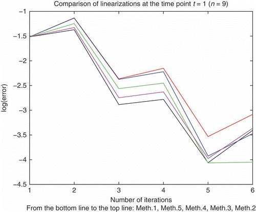
In the following, we compare graphically the linearization schemes in Figure 3 and shall discuss the best techniques.

Figure 3. The numerical errors of the different linearization techniques.

Remark 5. In this example, we have shown that higher non-linearity does not affect the efficiency of the linearization methods. This means that the accuracy of the modified linearized model does not affect the correctness of the full non-linear model. Here, the number of iteration steps and the number of time partitions are optimal with a second-order integration scheme. More iteration steps achieve the same results; see also [52].

4.3. Plasma reactor simulations: simplified model for the collision process

For collision processes in plasma reactors, it is very important to obtain the rate of each species (see [1]). We apply a simple reactive model and assume short distances to neglect the spatial behaviour of each species. We deal with two species involved in the reaction system and assume non-linearity in the reaction parts. An efficient linearization scheme is applied together with an iterative splitting scheme.

For the general reaction of A and B particles, we have

$3A+B\to A_{2}B+A.$

This reaction can be modelled as a non-linear differential equation:

(57) ${\mathrm{\partial }}_t{c}_a={\mathrm{\partial }}_t{c}_b=-k_{AB}{c}_a^2{c}_b-k_A{c}_a$(57)

where we assume a Maxwellian distribution with a common temperature T, and the rate constant $k_{AB}$ is given by $k_{AB}={\int }_0^{\mathrm{\infty }}{f}_m{v}_r{\sigma }_{AB}4\pi v_R^2\mathrm{d}{v}_R$.

We assume the dominant reaction is with species B, so that we can simplify:

(58) ${\mathrm{\partial }}_t{c}_a=-k_{AB}{c}_a^3--k_A{c}_a,t\in [0,T]$(58)

where we have initial conditions $c_a(0)=c_{a0}=1.0$, and the reaction rates are $k_{AB}=0.01$, $k_A=0.004$. The end time is given by $T=10.0$.

In Table 4, we have compared the optimal linearization methods (see Algorithm 41) for the non-linear equation (58) with $\alpha =3$, and the exact solution given in Section 3.1. We present the absolute error with respect to the exact solution at the time point $t=10$.

Table 4. Numerical errors of the optimal linearization technique 4).

$n_{\mathrm{i}\mathrm{t}}$	$n_{\mathrm{i}\mathrm{n}\mathrm{t}}$	$n_{\mathrm{t}\mathrm{s}}$	4)
1	1	1000	8.0852e-2
1	10	100	8.0852e-2
1	100	10	8.0852e-2
2	1	1000	5.1843e-3
2	10	100	4.6017e-4
2	100	10	4.5785e-5
3	1	1000	4.5400e-4
3	10	100	4.0729e-6
3	100	10	4.0599e-8
4	1	1000	1.4512e-5
4	10	100	1.3147e-8
4	100	10	2.1281e-11
5	1	1000	7.6057e-7
5	10	100	5.6436e-11
5	100	10	1.3809e-11
6	1	1000	1.6326e-8
6	10	100	8.0876e-12
6	100	10	7.9682e-12

Table 5. Physical parameters.

Pressure in the chamber	$p={9.810}^{-2}-2$ mbar
Precursor temperature	$T_{\mathrm{p}\mathrm{r}\mathrm{e}\mathrm{c}\mathrm{u}\mathrm{r}\mathrm{s}\mathrm{o}\mathrm{r}}=71.5deg\mathrm{C}$
Velocity (argon gas)	$v=30.0$ cm${\hspace{0.17em}}^3$/min
Inflow velocity of the precursor gas	$v_{\mathrm{i}\mathrm{n}\mathrm{f}\mathrm{l}\mathrm{o}\mathrm{w}}=0.60$ cm${\hspace{0.17em}}^3/$min

In Table 4, we have applied $n_{it}$ number of iterations and $n_{int}$ number of intervals (based on the improvement with method 6)) and $n_{ts}$ number of time-steps per interval. The physical parameters of the real-life experiments are given in Table 5.

In Figure 4, we see graphically the accuracy of the linearization schemes and do not see any differences between the linearized and non-linearized model.

Figure 4. x-axis: Time scale, y-axis: concentration, numerical solution and exact solution coincide in the same line.

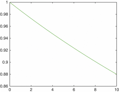
Remark 6. Based on the efficient second-order linearization scheme, we can apply such schemes to the collision kinetics of two particles. By applying multiple iteration steps we obtain more accurate results, where at the end the computer accuracy of our MATLAB software is attained. The efficiency of a fast iterative scheme for ODEs is obtained by alternating between each operator (see [52]). Here, we verified that we can apply the modified linearized model instead of the full non-linear model without any loss of accuracy.

4.4. Plasma reactor simulations: model for the transport and collision process of TiC deposition

We deal with a deposition model based on TiC, while the underlying titanium precursor (tetraethyltitanium), which leads to the deposition of TiC, is given by (see also [53]):

(59) $\mathrm{T}\mathrm{i}({\mathrm{C}\mathrm{H}}_2{\mathrm{C}\mathrm{H}}_3{)}_4\to \cdot {\mathrm{T}\mathrm{i}(\mathrm{C}\mathrm{H}}_2{\mathrm{C}\mathrm{H}}_3{)}_3+\cdot {\mathrm{C}\mathrm{H}}_2{\mathrm{C}\mathrm{H}}_3$(59)

(60) ${\mathrm{T}\mathrm{i}(\mathrm{C}\mathrm{H}}_2{\mathrm{C}\mathrm{H}}_3{)}_3\to \ddot{\mathrm{T}}\mathrm{i}(\mathrm{C}{\mathrm{H}}_2{\mathrm{C}\mathrm{H}}_3{)}_2+\cdot {\mathrm{C}\mathrm{H}}_2{\mathrm{C}\mathrm{H}}_3$(60)

(61) $\ddot{\mathrm{T}}{\mathrm{i}(\mathrm{C}\mathrm{H}}_2{\mathrm{C}\mathrm{H}}_3{)}_2\to \cdot \ddot{\mathrm{T}}{\mathrm{i}\mathrm{C}\mathrm{H}}_2{\mathrm{C}\mathrm{H}}_3+\cdot {\mathrm{C}\mathrm{H}}_2{\mathrm{C}\mathrm{H}}_3$(61)

so the final reaction is

(62) $2\stackrel{\mathrm{..}}{\text{T}}{\text{iCH2CH}}_3\to 2\text{TiC}+2{\text{CH}}_{\text{4}}+{\text{H}}_2$(62)

We compare this with a set-up for the physical experiment, including the bias voltage of the electric field, which is simulated as a retardation to the species. Such simulations allow validating our linearized reaction model given in Equation (62).

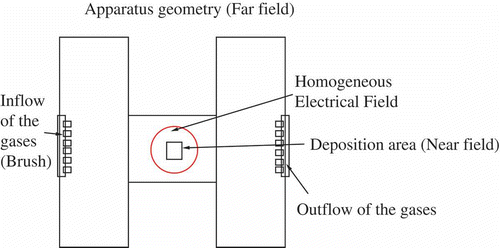
In the following numerical simulations, we simulate the near-field model, see Equation (1), for the deposition area (see Figure 5).

Figure 5. Spatial domain of the PE-CVD apparatus.

Such a contrast to the near field allows specifying the situation in the whole apparatus.

For the physical experiment, we have the following parameters:

Based on the approximation scheme, we carry out a simulation to derive the mathematical parameters.

For different physical situations, we can use the following mathematical parameters; see Table 6.

Table 6. Computed and experimental fitted parameters with UG simulations.

Power [W]	Bias [V]	$R_{\mathrm{C}}$ at material 1	$R_{\mathrm{T}\mathrm{i}}$ at material 2	Ratio (C:Ti) (numerical)
300	0	${0.110}^{-4}$	${2010}^{-4}$	$5.5:1.5=3.6$
600	0	${1.010}^{-4}$	${2010}^{-4}$	$4.4:1.5=2.93$
900	0	${1.510}^{-4}$	${2010}^{-4}$	$3.8:1.5=2.53$
300	–10	${2.810}^{-4}$	${2010}^{-4}$	$3.1:1.5=2.066$
600	–10	${1.010}^{-15}$	${2010}^{-4}$	$5.7:1.5=3.8$
900	–10	${1.010}^{-15}$	${6010}^{-4}$	$5.7:05=11.4$

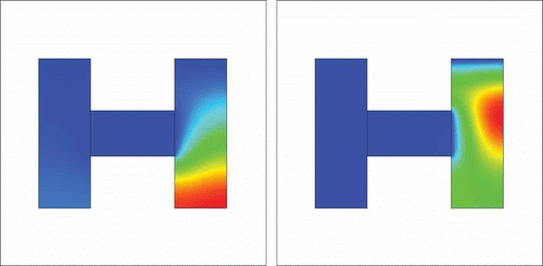
In Figures 6 and 7, we present an example of the concentration of two inflow sources $x_{\mathrm{T}\mathrm{i}},y_{\mathrm{T}\mathrm{i}}=(35,190)$ and $x_{\mathrm{T}\mathrm{i}},y_{\mathrm{T}\mathrm{i}}=(215,190)$. The velocity is that perpendicular to the apparatus.

Figure 6. Two inflow sources $x_{\mathrm{T}\mathrm{i}},y_{\mathrm{T}\mathrm{i}}=(35,190)$ and $x_{\mathrm{T}\mathrm{i}},y_{\mathrm{T}\mathrm{i}}=(215,190)$ with perpendicular velocity and 100 time-steps, with the ratio between C and Ti equal to 3.6.

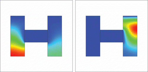
Figure 7. Two inflow sources $x_{\mathrm{T}i},y_{\mathrm{T}\mathrm{i}}=(35,190)$ and $x_{\mathrm{T}\mathrm{i}},y_{\mathrm{T}\mathrm{i}}=(215,190)$ with perpendicular velocity and 150 time-steps, with the ratio between C and Ti equal to 3.6.

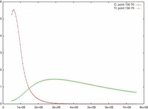
Figure 8 shows the deposition rates of two inflow sources $x_{\mathrm{T}\mathrm{i}},y_{\mathrm{T}\mathrm{i}}=(35,190)$ and $x_{\mathrm{T}\mathrm{i}},y_{\mathrm{T}\mathrm{i}}=(215,190)$ with perpendicular velocity and after 150 time-steps.

Figure 8. Deposition rates in the case of two point sources, x = 35,215, y = 190, with perpendicular velocity and 150 time-steps, with the ratio between C (+ line) and Ti (x line) equal to 3.6.

Remark 7. In the numerical simulations, there was a good fit with the experimental data, which validates the new linearized model. The optimal and effective linearization technique based on the trapezoidal rule is applied. The modified simulation model is as accurate as the full model, and it is simpler to implement the linearized reaction parts of the model problem, where they can then be treated as a system of linear ODEs. For practical reasons, it makes sense to save computational time, while reducing the model, although this must be done with care and with respect to polynomial non-linearities. At least, using the modified linearized model, we were able to find the mixture of flow regimes that provides the optimal deposition.

5. Conclusion and discussion

A modelling problem was modified using linearization and iterative techniques. Although the non-linear parts of the equations were delicate, we could use embedded linearization techniques and thus reduce the complexity of the model. More accurate modelling solutions are obtained with higher-order linearization techniques, e.g. quadrature rules. An optimal combination of time-step size, number of iterations and quadrature rules turned out to be the use of the trapezoidal rule or Simpson’s rule with less than 3–5 iterative steps and large time-steps. First, we applied this to a PE-CVD apparatus and were able to verify the new linearized model by comparing our theoretical results with those of experiment. In the future, we also will take into account the non-linear transport and scattering terms for the models.

Appendix

In this appendix, we present the applied splitting schemes used to reduce the order of the non-linear differential equations to linearized differential equations (see [44]). Such methods can be considered as MOR methods, which replace the original system (non-linear ODEs) by an approximating system (linear ODEs) with smaller dimensions of the solution space.

General iterative scheme

In the following, we consider splitting methods to efficiently solve complicated differential equations.

We concentrate on linearized time-dependent differential equations and present an iterative method (the iterative operator splitting method).

The contributions are to derive an efficient time-dependent scheme and embed this in higher-order iterative schemes. Based on the fixed point methods of the iterative schemes, we can also deal with non-linear differential equations, which are linearized.

Furthermore, we apply quadrature rules of higher order and embed such linearization techniques in the splitting method to accelerate the solver process.

The general iterative scheme is

(A1) $\frac{\mathrm{d}{U}_i}{\mathrm{d}t}=P(t)U_i+Q(t)U_{i-1}+F(t)$(A1)

(A2) $U_i(t^n)=U(t^n)\mathrm{f}\mathrm{o}\mathrm{r}i=1,2,\dots ,m$(A2)

where $P$ and $Q$ are time-dependent matrices $A(t)=P(t)+Q(t)$ of the splitting scheme.

We apply the general iterative scheme to the GLCS (39)–(40):

(A3) $\frac{\mathrm{d}U}{\mathrm{d}t}=A(t)U(t)+B(t)V(t)$(A3)

(A4) $\frac{\mathrm{d}\tilde{U}}{\mathrm{d}t}=C(t)U(t)+D(t)V(t)$(A4)

where $F(t)=B(t)V(t)$ is the right-hand side of (A6).

Later, we connect the underlying operator splitting scheme with that of the theory of linear control systems as fast solver methods.

Linear control systems are based on the following equations:

(A5) $\frac{\mathrm{d}u}{\mathrm{d}t}=Au(t)+Bv(t)$(A5)

where $A\mathrm{a}\mathrm{n}\mathrm{d}B$ are bounded and linear operators.

Such systems are discussed in [29,30,54,55].

Convergence of the iterative splitting method

The following algorithm is based on an iteration with a fixed splitting discretization step-size $\tau$. We solve the following subproblems consecutively for $i=1,2,\dots ,m$ (cf [56]) in the time interval $[t^n,t^{n+1}]$.

(A6) $\frac{\mathrm{d}{U}_i}{\mathrm{d}t}=P(t)U_i+Q(t)U_{i-1}+F(t)$(A6)

(A7) $U_i(t^n)=U(t^n),\mathrm{f}\mathrm{o}\mathrm{r}i=1,2,\dots ,m$(A7)

where $U_i(t)=(u_i(t),u_{i+1}(t){)}^t$ and $U_0(t^{n+1})=\equiv 0$ is the starting solution at the initial iteration $i=1$ and $U^n=U(t^n)$ is the known split approximation at time $t=t^n$. The split approximation at time $t=t^{n+1}$ is defined to be $U^{n+1}=U_m(t^{n+1})$. The matrices are

(A8) $P(t)=\left[\begin{array}{cc}{A}_1(t)& 0\\ A_1(t)& A_2(t)\end{array}\right],Q(t)=\left[\begin{array}{cc}0& A_2(t)\\ 0& 0\end{array}\right],F(t)=\left[\begin{array}{c}F(t)\\ F(t)\end{array}\right]$(A8)

Furthermore, we assume linear-bounded operators, $A_1(t),A_2(t),B(t):X(0,T)\to X(0,T)$, and that these operators and their sums are generators of an appropriate semigroup.

In the following, we will analyse the convergence and the rate of the convergence of the method (A6), where m tends to infinity.

Theorem 2. Let us consider the abstract Cauchy problem in a Banach space X(0,T) × X(0,T),

(A9) $\frac{d\mathrm{U}}{d\mathrm{t}}=\mathrm{A}(\mathrm{t})\mathrm{U}+\mathrm{F}(\mathrm{t})$(A9)

(A10) ${\mathrm{U}(\mathrm{t}}^{\mathrm{n}})={\mathrm{U}(\mathrm{t}}^{\mathrm{n}})$(A10)

where $\mathrm{A}(\mathrm{t})=\mathrm{P}(\mathrm{t})+\mathrm{Q}(\mathrm{t})$ and $\mathrm{A}(\mathrm{t}),\mathrm{P}(\mathrm{t}),\mathrm{Q}(\mathrm{t}):{\mathbf{X}}^2(\mathrm{t})\to {\mathbf{X}}^2(\mathrm{t})$ are given linear-bounded operators which are generators of an appropriate semigroup and $U(0)\in {\mathbf{X}}^2(0,T)$ is a given element. We assume that ${\int }_0^{\mathrm{T}}\mathrm{P}(\mathrm{s})d\mathrm{s}$, ${\int }_0^{\mathrm{T}}\mathrm{Q}(\mathrm{s})d\mathrm{s}$ can be approximated in the ith iteration scheme to order ${\mathrm{O}(\tau }_{\mathrm{n}}^{\mathrm{i}})$, for example,with the Magnus expansion in Section 3.2. The iteration process (A6) for $i=1,2,\dots ,m$ is then consistent with the order of ${\mathrm{O}(\tau }_{\mathrm{n}}^{\mathrm{m}})$.

Proof. Let us consider the iteration (A6) on the subinterval $[t^n,t^{n+1}]$. We use the notation $\mathbf{X}(0,T{)}^2$ for the product space $\mathbf{X}(0,T)\times \mathbf{X}(0,T)$ endowed with an appropriate Banach norm $||\cdot ||$ for vectors and also with the induced operator norm $||\cdot ||$.

The solution to the differential equation is

(A11) $U_i=K{U}_{i-1}+L$(A11)

(A12) $KU(t)={\int }_{t^n}^{t}exp({\int }_s^{t}P(\tilde{s})\mathrm{d}\tilde{s})Q(s)U(s)\mathrm{d}s$(A12)

(A13) $L=exp({\int }_s^{t}P(\tilde{s})\mathrm{d}\tilde{s})U(t^n)+{\int }_{t^n}^{t}exp({\int }_s^{t}P(\tilde{s})\mathrm{d}\tilde{s})F(s)\mathrm{d}s$(A13)

where $t\in [t^n,t^{n+1}]$ and $n=1,\dots ,N-1$ are the finite time intervals, and ${\tau }_n=t^{n+1}-t^n$ is the time-step.

If we apply the Magnus expansion to the time-dependent operators, we obtain the linear Volterra convolution operator with a continuous matrix-valued kernel,

(A14) $KU(t)=k\circ U(t)={\int }_{t^n}^{t}k(t-s)U(s)\mathrm{d}s$(A14)

(A15) $k(t)=exp({\int }_{t^n}^{t}P(\tilde{s})d\tilde{s})Q(t^n),$(A15)

where $t\in [t^n,t^{n+1}]$.

Then for finite time intervals, there is a constant C such that $||k||\le C$, and the convergence is

(A16) $||U-U_i||\le \frac{(C{\tau }_n{)}^m}{m!}||U-U_0||$(A16)

The proof is given in [57,58].

References

- M.A. Lieberman and A.J. Lichtenberg, Principle of Plasma Discharges and Materials Processing, 2nd ed., Wiley-Interscience, Hoboken, NJ, 2005.
- M. Ohring, Materials Science of Thin Films, 2nd ed., Academic Press, San Diego, CA, 2002.
- J. Geiser, V. Buck, and M. Arab, Model of PE-CVD apparatus: Verification and simulations, Math. Probl. Eng. (2010), Article ID 407561.
- T.K. Senega and R.P. Brinkmann, A multi-component transport model for non-equilibrium low-temperature low-pressure plasmas, J. Phys. D Appl. Phys. 39 (2006), pp. 1606–1618.
- J. Geiser and R. Roehle, Simulation of a multi-component transport model for the chemical reaction of a CVD-process, WASET, EEEng 2 (2) (2008), pp. 86–94.
- H. Neunzert and J. Struckmeier, Particle methods for Boltzmann equation, Acta Numer. (1995), pp. 417–457.
- C. Cercignani, The Boltzmann Equation and Its Applications, Springer-Verlag, Berlin, 1987.
- M.K. Gobbert and C.A. Ringhofer, An asymptotic analysis for a model of chemical vapor deposition on a microstructured surface, SIAM J. Appl. Math. 58 (1998), pp. 737–752.
- C. Ringhofer, Dissipative discretization methods for approximations to the Boltzmann equation, Math. Models Methods Appl. Sci. 12 (2001), pp. 133–148.
- P.A. Raviart, An analysis of particle methods, in Numerical Methods in Fluid Dynamics, Lecture Notes in Math, Vol. 1127, F. Brezzi, ed., Springer-Verlag, Berlin, 1985, pp. 243–324.
- R. Hockney and J. Eastwood, Computer Simulation Using Particles, Taylor and Francis, New York, 1988.
- S. Rjasanow and W. Wagner, A generalized collision mechanism for stochastic particle schemes approximating Boltzmann type equations, Comput. Math. Appl. 35 (1998), pp. 165–178.
- M. Asadzadech and A. Sopasakis, Convergence of a hp-streamline diffusion scheme for VlasovFokkerPlank, Math. Models. Methods. Appl. Sci. 17 (2007), pp. 1159–1182.
- S. Rjasanow, T. Schreiber, and W. Wagner, Reduction of the number of particles in the stochastic weighted particle method for the Boltzmann equation, J. Comput. Phys 145 (1) (1998), pp. 382–405.
- P. Crispel, P. Degond, and M.H. Vignal, A plasma expansion model based on the full Euler–Poisson model, Math. Models. Methods. Appl. Sci. 17 (2007), pp. 1129–1158.
- S. Motta and J. Wick, A new numerical methods for kinetic equations in several dimensions, Computing 46 (1991), pp. 223–232.
- S. Motta, A new formulation and gauge invariance of the MW-CRF method for kinetic equations, Math. Comput. Model. 36 (4–5) (2002), pp. 403–410.
- S. Motta, Energy conservation property of the MW-CRF deterministic particle method, Appl. Math. Lett. 16 (2003), pp. 287–292.
- C. Bianca, F. Pappalardo, and S. Motta, The MWF method for kinetic equations system, Comput. Math. Appl. 57 (2009), pp. 831–840.
- C. Bianca and S. Motta, The MWF method: A convergence theorem for homogeneous one-dimensional case, Comput. Math. Appl. 58 (2009), pp. 579–588.
- J. Wick, Numerical approaches to the kinetic semiconductor equation, Computing. 52 (1994), pp. 39–49.
- Y. Chen. Model Order Reduction for Nonlinear Systems. M.S. Thesis, Massachusetts Institute of Technology, Cambridge, MA, September 1999.
- L. Feng, Review of model order reduction methods for numerical simulation of nonlinear circuits, Appl. Math. Comput. 167 (2005), pp. 576–591.
- M. Rewienski and J. White. Improving trajectory piecewise-linear approach to nonlinear model order reduction for micromachined devices using an aggregated projection basis, in Technical Proceedings of the 2002 International Conference on Modeling and Simulation of Microsystems, Chapter 3: System Level Modeling of MEMS, San Juan, Puerto Rico, 2002, pp. 128–131.
- M. Rewienski. A trajectory piecewise-linear approach to model order reduction of nonlinear dynamical systems. Ph.D. Thesis, Massachusetts Institute of Technology, Cambridge, MA, June 2003.
- J. Geiser and R. Roehle, Kinetic processes and phase-transition of CVD processes for Ti2SiC3, J. Convergence Inf. Technol. 5 (6) (2010), pp. 9–32.
- J. Geiser, Computing exponential for iterative splitting methods: Algorithms and applications, J. Appl. Math. (2011), Article ID 193781.
- G.M. Kepler, H.T. Tran, and H.T. Banks, Reduced order model compensator control of species transport in a CVD reactor, Optimal Control Appl. Methods. 21 (1999), pp. 143–160.
- P.J. Antsaklis and A.N. Michel, Linear Systems, McGraw-Hill, New York, 1997.
- L. Zadeh and C. Desoer, Linear System Theory. The State Space Approach, McGraw-Hill, New York, 1963.
- B. Chapman, Glow Discharge Processes. Sputtering and Plasma Etching, John Wiley & Sons, New York, 1980.
- N. Morosoff, Plasma Deposition, Treatment and Etching of Polymers, Academic Press, Boston, MA, 1990.
- F. Langlais, F. Loumagne, D. Lespiaux, S. Schamm, and R. Naslain, Kinetic processes in the CVD of SiC from CH3SiCl3-H2 in a vertical hot-wall reactor, J. Phys. IV Colloque C5 Suppl J. Phys II. 5 (1995), pp. 105–115.
- P. Favia, E. Sardella, R. Gristina, A. Millella, and R. D’Agostino, Functionalization of biomedical polymers by means of plasma processes: Plasma treated polymers with limited hydrophobic recovery and PE-CVD of COOH functional coatings, J. Polym. Sci. Technol. 15 (2) (2002), pp. 341–350.
- H. Rouch. MOCVD Research Reactor Simulation. Proceedings of the COMSOL Users Conference 2006, Paris, France, 2006.
- V.A. Kadetov. Diagnostics and modeling of an inductively coupled radio frequency discharge in hydrogen. Ph.D. thesis, Ruhr University of Bochum, Germany, 2004.
- J. Geiser and M. Arab, Porous media-based modeling of PE-CVD apparatus: Electrical fields and deposition geometries, Spec. Topics Rev. Porous Media 1 (3) (2010), pp. 215–229.
- L. Rudniak, Numerical simulation of chemical vapour deposition process in electric field, Comput. Chem. Eng. 22 (1998), pp. 755–758.
- J. Geiser, Multiscale modeling of chemical vapor deposition (CVD) apparatus: Simulations and approximations, Spec. Issue Multiscale Simul. oft Matter. Polym. 5 (1) (2013), pp. 142–160.
- A. Taflove and S.C. Hagness, Computational Electrodynamics: The Finite-Difference Time-Domain Method, 3rd ed., Artech House, Norwood, MA, 2005.
- P. Knabner and L. Angerman, Numerical Methods for Elliptic and Parabolic Partial Differential Equations, Springer-Verlag, New York, 2003.
- J. Geiser, Iterative Splitting Methods for Differential Equations, Chapman & Hall/CRC, Boca Raton, FL, 2011.
- B. Gustafsson, High-Order Difference Methods for Time Dependent PDE, Springer-Verlag, Berlin, 2008.
- C.T. Kelley, Iterative Methods for Linear and Nonlinear Equations, Series: Frontiers in Applied Mathematics, Vol. 16, SIAM, Philadelphia, PA, 1995.
- J. Geiser, Iterative operator-splitting methods for nonlinear differential equations and applications, Numer. Methods Partial Differential Equations 27 (5) (2011), pp. 1026–1054.
- A.D. Polyanin and V.F. Zaitsev, Handbook of Exact Solutions for Ordinary Differential Equations, 2nd ed., Chapman & Hall, Boca Raton, FL, 2002.
- S. Blanes, F. Casas, J.A. Oteo, and J. Ros, The Magnus expansion and some of its applications, Phys. Rep. 470 (5–6) (2009), pp. 151–238.
- S. Blanes and P.C. Moan, Fourth- and sixth-order commutator-free Magnus integrators for linear and nonlinear dynamical systems, Appl. Numer. Math. 56 (2006), pp. 1519–1537.
- F. Casas and A. Iserles, Explicit Magnus expansions for nonlinear equations, J. Phys. A Math. Gen. 39 (2006), pp. 5445–5461.
- J. Geiser, Computing exponential for iterative splitting methods, J. Appl. Math. 2011 (2011), Article ID 193781.
- D. Zwillinger (ed.), Bernoulli equation chapter II.A, 37, in Handbook of Differential Equations, 3rd ed., Academic Press, Boston, MA, 1997, pp. 157–158.
- J. Geiser, Consistency of iterative operator-splitting method, Theory and Appl. published online. doi:10.1002/num. 20422
- J. Geiser and R. Roehle, Kinetic processes and phase-transition of CVD processes for Ti2SiC3, J Convergence Inf. Technol. 5 (6) (2010), pp. 9–32.
- R. Bellman, Introduction to Matrix Analysis, Mcgraw-Hill, New York, 1960.
- J.S. Respondek, Approximate controllability of the nth order infinite dimensional systems with controls delayed by the control devices, Int. J. Syst. Sci. 39 (8) (2008), pp. 765–782.
- I. Farago and J. Geiser. Iterative Operator-Splitting Methods for Linear Problems. Preprint No. 1043 of the Weierstrass Institute for Applied Analysis and Stochastics, Berlin, Germany, June 2005.
- U. Miekkala and O. Nevanlinna, Convergence of dynamic iteration methods for initial value problems, SIAM J. Sci. Stat. Comput. 8 (1987), pp. 459–482.
- S. Vandewalle, Parallel Multigrid Waveform Relaxation for Parabolic Problems, B.G. Teubner, Stuttgart, 1993.