Modelling and experimental validation of the deflection of a leveller for hot heavy plates

Abstract

In order to successfully automate levelling processes, in particular for heavy plates, the deflection of the leveller has to be compensated based on a deflection model. In this work, a detailed mathematical deflection model of a hot leveller with bending mechanism and its experimental validation are presented. The roll intermesh profiles are calculated based on the deflection of the work rolls that are elastically supported by support rolls, frames, posts and adjustment screws. The deflection model is suited to compensate the effect of deflection on the roll intermesh and the plate flatness as well as to assess the loads of critical parts, for example the support rolls. A new experimental design to measure the deflection of a leveller is presented and successfully applied for model validation. The work roll deflection is measured directly by means of displacement sensors that are inserted in cut-outs of test plates. These test plates are modelled as linear elastic stripes. For normal load levels, the relative accuracy (repeatability) of the roll intermesh prediction of the model is better than 0.08 mm.

Keywords:

• hot rolling mills
• precision leveller
• deflection modelling
• deflection measurement

1. Introduction

In hot rolling mills, levellers are applied to reduce residual stresses and flatness defects of hot-rolled steel plates. To reduce developable flatness defects, alternating bending and the plastification of the plate at each roll have to be precisely controlled in longitudinal direction of the plate. At the same time, the roll intermesh along the plate width has to be controlled to reduce non-developable flatness defects. Moreover, levelling forces up to several meganewtons may occur that lead to elastic deformations of the machine, especially when levelling heavy plates. For quality reasons, these deformations have to be compensated. Furthermore, overloading must be avoided because it may cause expensive failure of leveller equipment. In order to increase quality and throughput, the automation of levelling processes is promoted both by manufacturers and by operators of levellers. In general, automation systems of levellers have to cope with the challenges mentioned above.

For rolling equipment, the deflection of the machine is usually compensated by means of additional set points for the references of the position controllers of the main adjustment variables. For this, the set point is calculated with a deflection model of the machine. If the load can be fully measured online, the deflection compensation can be performed dynamically in terms of feedback control. In the context of automatic gauge control, this method is often referred to as gauge meter control [1]. Typically, the exact load distribution along the rolls of rolling mills or levellers is not available in real time. In this case, based on a process model and the deflection model, the additional set point can be applied in a feedforward sense. However, accurate models of both the process and the deflection are required.

Various models of the levelling process can be found in the literature; some of them may serve as a basis for leveller automation. However, the deflection of the leveller is just marginally considered and often neglected. Levelling models for sheet metal, including elaborated material models with work hardening, are presented in [2] and [3]. The latter also describes the basics of levelling non-developable flatness defects by means of work roll bending. An analytical model that may be used to analyse the influence of lateral work roll profiles on non-developable flatness defects is provided in [4]. In all the aforementioned works, the deflection of the leveller structure is not considered but the work roll positions are used as geometrical boundary conditions to solve the deformation problem of the levelled sheet. In [5], a levelling model with coupled deflection of each work roll is discussed. However, the model does not provide a roll deflection profile. Examples of successful model-based leveller automation are given in [6] and [7]. As they focus on levelling models and strategies, they mention the deflection of the leveller only rudimentary.

For recently built levellers, deflection models may be available from an integrated CAD/FEM design process, cf. the leveller described in [8]. Such tailored autogenerated models are usually not available for machines that were built some decades ago. However, these old machines may still be in use if they are regularly maintained and revamped.

In addition to a lack of appropriate deflection models of levellers, the deflection of a real leveller is difficult to measure. Ideally, the applied roll loads and the resulting deflections should be measured directly. In [9], a measurement procedure for presses is standardized. Here, special hydraulic cylinders are used to load the frame that carries the die. Thus, the loaded area is relatively small, test loads can be easily applied and the corresponding deflection can be easily measured close to the loads. In contrast to the loads in a press, the levelling load is distributed over a considerable width of several rolls. Creating a load distribution similar to a real levelling load in a controlled manner, for instance with an array of hydraulic cylinders, would be laborious. Additionally to the large number of necessary cylinders, it would be difficult to design the contact between cylinders and work rolls, whose surfaces should not carry concentrated forces. Moreover, the upper and the lower work rolls do not directly oppose each other. The latter fact also prevents the application of known methods from, for example rolling mills, where the upper and the lower work rolls are brought into contact by means of the adjustment cylinders. In this way, the mill stretch can be identified in the form of a force–displacement curve. Clearly, this method does not directly include the identification of a deflection model for roll gap profiles, cf. [10]. An experimental approach to measure the curvature of the plate by means of strain gauges right during the levelling process is presented in [11]. They use their measurement results to validate a levelling model. Clearly, uncertainties of the deflection model of the leveller are thus erroneously incorporated into the model of the plate and vice versa.

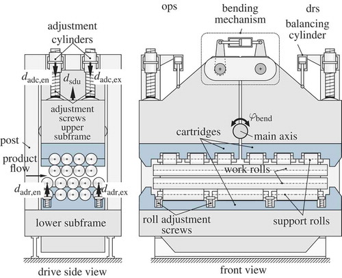
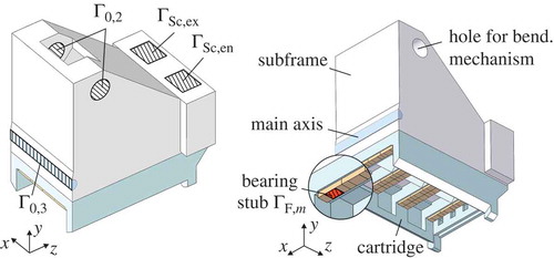
In this work, a detailed deflection model of a reversing 9-roll hot leveller with bending mechanism (cf. Figure 1) and the experimental model validation are presented. The model allows for an arbitrary adjustment of the support rolls and can thus be easily transferred to levellers with more degrees of freedom. A new experimental design was developed for validation purposes. The deflection model is suited to analyse the effect of deflection on the roll intermesh and the flatness of the plate. Moreover, it can be used to assess the loads of critical parts, for example the support rolls. The model grounds on basic geometrical and mechanical properties of the involved parts; finite element methods were occasionally used to parameterize and verify parts of the model. Some possibilities to use the model for active deflection compensation are given in [12] and [13]. However, these publications lack a comprehensive derivation and a solid validation of the model. These issues are the main contribution of the current paper.

Figure 1. The considered 9-roll hot leveller with bending mechanism.

The paper is organized as follows: in Section 2, the deflection model of the leveller is derived. Additionally, a basic model of a test plate is presented that is used for the validation experiments. In Section 3, the design and the procedure of these experiments are explained. Finally, the validation results are presented. In Section 4, conclusions are drawn and an outlook on further work is given. In the ‘Appendix’ section, the relations of the kinematics of the leveller are summarized.

2. Deflection model

2.1. Adjustment variables

The considered hot leveller features the following main adjustment variables: the adjustment screws define the vertical reference position d_sdu of the upper subframe; all the following displacements of the upper subframe are relative to this position. The upper subframe can be vertically positioned and also tilted with respect to the lateral axis by means of adjustment cylinders (d_adc,en, d_adc,ex). To control the bending line of the upper work rolls, the upper subframe is split into two halves. These halves can be tilted with respect to each other by the angle φ_bend by means of a hydraulically actuated bending mechanism, cf. Figure 1. The compliance of the bending mechanism itself is not covered in this work because in [14], it is shown how this compliance can be automatically compensated by means of feedback control. Furthermore, the entry and exit rolls can be individually adjusted by d_adr,en and d_adr,ex, respectively.

2.2. Coordinate systems

The origin $d_{\mathrm{s}\mathrm{d}\mathrm{u}}=0$ of the screw displacement is defined by the point where the upper vertices of the lower rolls and the lower vertices of the upper rolls lie on the same horizontal plane. Usually, the adjustment screws set the reference position of the upper frame in accordance with the height of the plate, that is $d_{\mathrm{s}\mathrm{d}\mathrm{u}}=h_{\mathrm{p}\mathrm{l}}$, cf. Figure 2. In this position, the work rolls would just touch the plate without causing any forces or deformations. The origin of the reference coordinate system $O{x}^0{y}^{0}z$ is set to the intersection point of the symmetry planes of the plate, cf. the drive side view in Figure 2. This coordinate system is suited to describe the deflection of the levelled plate. To describe the deflection of the upper (up) and lower (lo) work rolls, two additional coordinate systems $O{x}^{\mathrm{u}\mathrm{p}}{y}^{\mathrm{u}\mathrm{p}}z$ and $O{x}^{\mathrm{l}\mathrm{o}}{y}^{\mathrm{l}\mathrm{o}}z$ are introduced. Their origins are set to the horizontal centre planes of the work rolls; thus, $y^{\mathrm{u}\mathrm{p}}=y^0-\left(h_{\mathrm{p}\mathrm{l}}/2+r_{\mathrm{W}\mathrm{R}}\right)$ and $y^{\mathrm{l}\mathrm{o}}=-y^0-\left(h_{\mathrm{p}\mathrm{l}}/2+r_{\mathrm{W}\mathrm{R}}\right)$, with the work roll radius r_WR. The superscripts ‘up’ and ‘lo’ are omitted if the context does not require a differentiation between the upper and the lower frame.

Figure 2. Configuration of rolls and coordinate systems.

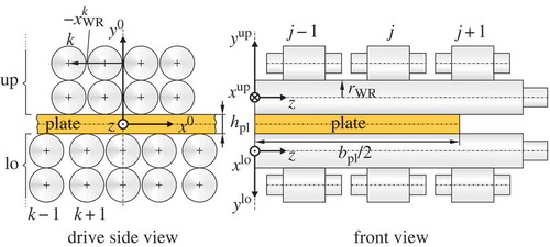
The 9 work rolls are indexed by k, beginning at the entry side with $k=1$. The support rolls are indexed by j, beginning at $z=0$. The number of support rolls associated with each work roll is 3. Furthermore, the edges of the support rolls are numbered by $i=1,\dots ,6$ in ascending order with increasing z coordinate, cf. Figure 3.

2.3. Assumptions

For the considered leveller, the configuration of the rolls and frames is symmetric with respect to the planes $x^0\text{-}{y}^0$ and $y^0\text{-}z$ shown in Figure 2. Usually, the leveller is symmetrically adjusted on the operator side (ops) and the drive side (drs). Assuming that the plate is symmetric as well, only the drive side of the leveller is considered for the deflection model.

For all machine components, linear elastic deformation with a constant Young’s modulus E is assumed. Generally, small deflections and linear geometric relations are supposed. The deflection of the leveller and the admissible operating range of the adjustment variables do not exceed a few millimetres, which is small compared to the dimensions of the leveller. The tilt and the bending adjustment only involve small rotational displacements of the upper subframe. Furthermore, these small rotational angles induce only negligible horizontal displacements of the roll centres. As a first approximation, it is assumed that the adjustment variables can be controlled exactly. In reality, the actual control accuracy of the adjustment actuators is about 50 μm.

Figure 3. Top: configuration of work and support rolls. Bottom: line loads and approximated concentrated forces acting on the work roll with simplified geometry.

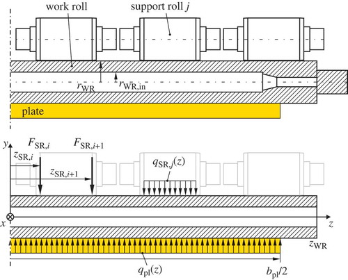
Figure 4. Reference position and position under load of a work roll in contact with a support roll.

2.4. Work roll deflection

In this section, differential equations for the bending line of a single work roll are developed. Figure 3 shows a work roll (WR) and the corresponding support rolls (SR). Along the direction x, the work rolls are supported by means of roller bearings at their journals. These bearings can freely move along the direction y and are thus neglected. The weight of the upper work rolls is balanced by disk springs and thus is negligible in this analysis.

Work rolls of hot levellers are usually cooled with water from the inside. They are therefore hollow with a bore radius of r_WR,in. For the deflection model, the simplified geometry of the work roll shown in the bottom view of Figure 3 is used. Moreover, the compression of the work roll and the support rolls due to ovalization and flattening is assumed to be small, in fact negligible compared to the deflection of the remaining structure, see also Section 2.6. Consequently, the radii of the work and support rolls, r_WR and r_SR, are constant. The areal moment of inertia of a cross section of the work roll is given by $I_{\mathrm{W}\mathrm{R}}=\pi (r_{\mathrm{W}\mathrm{R}}^4-r_{\mathrm{W}\mathrm{R},\mathrm{i}\mathrm{n}}^4)/4$. Moreover, with the constant Young’s modulus E, the constant bending stiffness reads as $K_{\mathrm{b},\mathrm{W}\mathrm{R}}=E{I}_{\mathrm{W}\mathrm{R}}$.

Figure 4 shows the simplified geometry of a support roll in contact with a work roll, both in the unloaded reference position and the position with non-zero adjustment under load. Here, $v_{\mathrm{S}\mathrm{R}}\left(z\right)$ is the vertical displacement of the support roll and $a{d}_{\mathrm{S}\mathrm{R}}\left(z\right)$ is the nominal adjustment of the support roll relative to the reference position. The displacement $v_{\mathrm{S}\mathrm{R}}\left(z\right)$ is the sum of the local deformation of the support roll itself and the deflection of the structures that support the support rolls, that is, their bearings, the subframes, etc. The nominal adjustment $a{d}_{\mathrm{S}\mathrm{R}}\left(z\right)$ is controlled by the adjustment variables of the leveller in terms of rigid body displacements, cf. Equations (A5) and (A6) in Appendix A. That is, $v_{\mathrm{S}\mathrm{R}}\left(z\right)$ is associated with the elastic deformation due to the loads and $a{d}_{\mathrm{S}\mathrm{R}}\left(z\right)$ with the actuators. According to Figures 3 and 4, on the interval $z\in \left[z_{\mathrm{S}\mathrm{R},i},z_{\mathrm{S}\mathrm{R},i+1}\right]$, $i=1,3,5$, the support roll deflection is related to the bending line $v_{\mathrm{W}\mathrm{R}}\left(z\right)$ of the work roll and the nominal adjustment $a{d}_{\mathrm{S}\mathrm{R}}\left(z\right)$ by

(1) $v_{\mathrm{S}\mathrm{R}}\left(z\right)=v_{\mathrm{W}\mathrm{R}}\left(z\right)-a{d}_{\mathrm{S}\mathrm{R}}\left(z\right).$(1)

The shape of the plate is thus directly defined by $v_{\mathrm{W}\mathrm{R}}\left(z\right)$.

Along the plate width $b_{\mathrm{p}\mathrm{l}}$, the work roll is loaded by the distributed levelling force $q_{\mathrm{p}\mathrm{l}}\left(z\right)$, where $q_{\mathrm{p}\mathrm{l}}\left(z\right)=0$ for $z>b_{\mathrm{p}\mathrm{l}}/2$, see Figure 3. Furthermore, the work rolls are loaded by the distributed contact forces $q_{\mathrm{S}\mathrm{R},j}\left(z\right)$ of their contact line with the support rolls, cf. the bottom view of Figure 3. The work roll is assumed to be in mechanical equilibrium, that is, the contact forces balance the levelling force.

The profile of the distributed contact forces $q_{\mathrm{S}\mathrm{R},j}\left(z\right)$ depends also on the local deformation of the support roll. However, modelling these local effects is a challenging task. For instance, consideration of the bending deflection profile of the support roll would require solving differential equations for each roll coupled with the equations for the work rolls. This would highly increase the complexity of the problem without significant improvement of the control performance because the available adjustment variables do not allow for a precise control of local effects anyway. To simplify the problem, the distributed contact force $q_{\mathrm{S}\mathrm{R},j}\left(z\right)$ is thus approximated by two concentrated forces $F_{\mathrm{S}\mathrm{R},i}$ and $F_{\mathrm{S}\mathrm{R},i+1}$ acting on the edges of the support roll, cf. the left support roll in Figure 3. This can be motivated by the following facts: first, the edges mainly bear the load of the work roll section between two support rolls. Second, as the edges of the support rolls are close to the bearings, they have a lower compliance than the surface points between them, see also Section 2.5.2. This may cause the support roll to partially lose contact with the bent work roll, particularly for non-zero bending adjustments. High edge loads are the consequence of this effect. For this analysis, it is thus accurate enough to couple the displacements of the work and support rolls at the edges of the support rolls.

The contact forces strictly have to be compressive forces. Consequently, the condition

(2) $F_{\mathrm{S}\mathrm{R},i}\ge 0$(2)

must hold for each contact force $\left(i=1,\dots ,6\right)$. The forces vanish if the contact between the work and the support roll is lost.

The assumption of small deflections qualifies the slender work rolls to be modelled as Euler–Bernoulli beams, cf. [15]. Thus, a fourth-order ordinary differential equation for the deflection of the work rolls can be derived as

(3) $K_{\mathrm{b},\mathrm{W}\mathrm{R}}\frac{{\mathrm{d}}^4}{\mathrm{d}{z}^4}{v}_{\mathrm{W}\mathrm{R}}\left(z\right)=q_{\mathrm{p}\mathrm{l}}\left(z\right),0\le z\le z_{\mathrm{W}\mathrm{R}}.$(3)

This boundary value problem (BVP) is supplemented by the following boundary conditions. At $z=z_{\mathrm{W}\mathrm{R}}$, boundary conditions for a free end are imposed (I) and symmetry conditions are formulated at $z=0$ (II), that is,

(4a) $\mathrm{I}:\frac{{\mathrm{d}}^2{v}_{\mathrm{W}\mathrm{R}}}{\mathrm{d}{z}^2}\left(z_{\mathrm{W}\mathrm{R}}\right)=0,\frac{{\mathrm{d}}^3{v}_{\mathrm{W}\mathrm{R}}}{\mathrm{d}{z}^3}\left(z_{\mathrm{W}\mathrm{R}}\right)=0.$(4a)

(4b) $\mathrm{I}\mathrm{I}:\frac{\mathrm{d}{v}_{\mathrm{W}\mathrm{R}}}{\mathrm{d}z}\left(0\right)=0,\frac{{\mathrm{d}}^3{v}_{\mathrm{W}\mathrm{R}}}{\mathrm{d}{z}^3}\left(0\right)=0.$(4b)

As the concentrated edge forces cause discontinuities of the shear forces in the work rolls, transition conditions for the positions $z_{\mathrm{S}\mathrm{R},i}$ can be derived in the form

(5a) $\frac{{\mathrm{d}}^n{v}_{\mathrm{W}\mathrm{R}}}{\mathrm{d}{z}^n}\left(z_{{ }^{\mathrm{S}\mathrm{R},i}}^{-}\right)=\frac{{\mathrm{d}}^n{v}_{\mathrm{W}\mathrm{R}}}{\mathrm{d}{z}^n}\left(z_{\mathrm{S}\mathrm{R},i}^{+}\right),n=0,1,2,$(5a)

(5b) $\frac{{\mathrm{d}}^3{v}_{\mathrm{W}\mathrm{R}}}{\mathrm{d}{z}^3}\left(z_{{ }^{\mathrm{S}\mathrm{R},i}}^{-}\right)=\frac{{\mathrm{d}}^3{v}_{\mathrm{W}\mathrm{R}}}{\mathrm{d}{z}^3}\left(z_{\mathrm{S}\mathrm{R},i}^{+}\right)-\frac{F_{\mathrm{S}\mathrm{R},i}}{K_{\mathrm{b},\mathrm{W}\mathrm{R}}}$(5b)

with $i=1,\dots ,6$. Here, $z_{\mathrm{S}\mathrm{R},i}^{+}$ and $z_{\mathrm{S}\mathrm{R},i}^{-}$ indicate the right- and the left-hand side limit at the respective position.

In order to calculate the deflection profiles $v_{\mathrm{W}\mathrm{R}}^k\left(z\right)$, $k=1,\dots ,9$, of all work rolls of the leveller, a BVP has to be solved that consists of nine differential equations in the form of Equation (3) with corresponding boundary and transition conditions (4) and (5). The differential equations of the work rolls are coupled by the plate because the right-hand side of Equation (3), that is, the distributed plate force, $q_{\mathrm{p}\mathrm{l}}^k\left(z\right)$, depends on the shape defined by the bending lines $v_{\mathrm{W}\mathrm{R}}^k\left(z\right)$ of all work rolls, $k=1,\dots ,9.$ Furthermore, the work rolls are coupled by the elastic frames because the force $F_{\mathrm{S}\mathrm{R},i}$, which appears in the transition condition (5b), generally depends on the deflection of all support roll edges of all work rolls. The force–deflection relations of the frames and the model of the plate are discussed in the following four sections.

2.5. Force–deflection relations of the frames

In this section, the force–deflection relations between the forces $F_{\mathrm{S}\mathrm{R},i}$ and the effective elastic deflections $v_{\mathrm{S}\mathrm{R}}\left(z_{\mathrm{S}\mathrm{R},i}\right)$ at the edges of the support rolls are derived. These effective deflections are briefly referred to as the deflection of the frame; however, they also include the deflection of the bearings, the subframes, the screws and the posts.

First, vectors are introduced which allow for a compact notation of the considered deflections and forces. An evaluation of Equation (1) at the locations $z_{\mathrm{S}\mathrm{R},i}$ of the edges $i=1,\dots ,6$ of the support rolls of the work roll k defines the deflection vector $v_{\mathrm{S}\mathrm{R}}^k$ of the support roll, the displacement vector $v_{\mathrm{W}\mathrm{R}}^k$ of the work roll and the vector of the nominal support roll adjustment ${ad}_{\mathrm{S}\mathrm{R}}^k$,

(6) $\underset{v_{\mathrm{S}\mathrm{R}}^k}{\underbrace{\left[\begin{array}{c}{v}_{\mathrm{S}\mathrm{R},1}^k\\ ⋮\\ v_{\mathrm{S}\mathrm{R},6}^k\end{array}\right]}}=\underset{v_{\mathrm{W}\mathrm{R}}^k}{\underbrace{\left[\begin{array}{c}{v}_{\mathrm{W}\mathrm{R}}^k\left(z_{\mathrm{S}\mathrm{R},1}\right)\\ ⋮\\ v_{\mathrm{W}\mathrm{R}}^k\left(z_{\mathrm{S}\mathrm{R},6}\right)\end{array}\right]}}-\underset{{ad}_{\mathrm{S}\mathrm{R}}^k}{\underbrace{\left[\begin{array}{c}a{d}_{\mathrm{S}\mathrm{R}}^k\left(z_{\mathrm{S}\mathrm{R},1}\right)\\ ⋮\\ a{d}_{\mathrm{S}\mathrm{R}}^k\left(z_{\mathrm{S}\mathrm{R},6}\right)\end{array}\right]}}.$(6)

By analogy, the vector $z_{\mathrm{S}\mathrm{R}}^k$ of the locations of the edges and the vector $F_{\mathrm{S}\mathrm{R}}^k$ of the edge forces are introduced. Note that all these vectors are elements of ${\mathbb{R}}^6$.

The vectors corresponding to either the upper or the lower frame can be combined to a column vector as well. The edge forces, for instances, are assembled in the form

(7a) $F_{\mathrm{S}\mathrm{R}}^{\mathrm{u}\mathrm{p}}=[F_{\mathrm{S}\mathrm{R}}^k]\in {\mathbb{R}}^{24},k\in \{2,4,6,8\},$(7a)

(7b) $F_{\mathrm{S}\mathrm{R}}^{\mathrm{l}\mathrm{o}}=[F_{\mathrm{S}\mathrm{R}}^k]\in {\mathbb{R}}^{30},k\in \{1,3,5,7,9\}.$(7b)

Figure 5. Nonconforming contact under load and typical force–deflection characteristic of the real machine, cf. [16].

By analogy to Equation (7), the vectors $v_{\mathrm{S}\mathrm{R}}^{\mathrm{u}\mathrm{p}}$, $v_{\mathrm{S}\mathrm{R}}^{\mathrm{l}\mathrm{o}}$, $v_{\mathrm{W}\mathrm{R}}^{\mathrm{u}\mathrm{p}}$, $v_{\mathrm{W}\mathrm{R}}^{\mathrm{l}\mathrm{o}}$, ${ad}_{\mathrm{S}\mathrm{R}}^{\mathrm{u}\mathrm{p}}$ and ${ad}_{\mathrm{S}\mathrm{R}}^{\mathrm{l}\mathrm{o}}$ can be defined.

The edge forces $F_{\mathrm{S}\mathrm{R},i}$ in Equation (5b) are the solution of the generally nonlinear vector-valued force–deflection relation

(8) $v_{\mathrm{S}\mathrm{R}}^{\nu }=s_{\mathrm{l}\mathrm{e}\mathrm{v}}^{\nu }\left(F_{\mathrm{S}\mathrm{R}}^{\nu }\right),\nu \in \left\{\mathrm{u}\mathrm{p},lo\right\},$(8)

subject to the contact condition (2),

(9) $F_{\mathrm{S}\mathrm{R}}^{\nu }={\left(s_{\mathrm{l}\mathrm{e}\mathrm{v}}^{\nu }\right)}^{-1}\left(v_{\mathrm{W}\mathrm{R}}^{\nu }-{ad}_{\mathrm{S}\mathrm{R}}^{\nu }\right),\nu \in \left\{\mathrm{u}\mathrm{p},\mathrm{l}\mathrm{o}\right\},$(9)

cf. Equations (6) and (7). Inserting Equation (9) into Equation (5b) shows the influence of the nominal adjustment on the work roll deflection.

2.5.1. Contact nonlinearities

Backlash, surface roughness or geometric deviations in the contact alignment or the surface shape may cause nonconforming contacts between the parts of the leveller. These nonconformities lead to nonlinear force–deflection curves of the real machine as shown in Figure 5 [16]. It is supposed that for forces greater than a calibration force $F_{\mathrm{c}\mathrm{a}\mathrm{l}}$, the contact surfaces conform and the force–deflection relations are approximately linear because they are dominated by the linear elastic material behaviour.

Applying this concept to the leveller, the force–deflection relation (8) may be written in the form

(10) $v_{\mathrm{S}\mathrm{R}}=\underset{v_{\mathrm{S}\mathrm{R},\mathrm{c}\mathrm{a}\mathrm{l}}}{\underbrace{s_{\mathrm{l}\mathrm{e}\mathrm{v}}\left(F_{\mathrm{S}\mathrm{R},\mathrm{c}\mathrm{a}\mathrm{l}}\right)}}+\underset{{\mathbf{S}}_{\mathrm{l}\mathrm{e}\mathrm{v}}}{\underbrace{{\left(\frac{\mathrm{\partial }{s}_{\mathrm{l}\mathrm{e}\mathrm{v}}}{\mathrm{\partial }{F}_{\mathrm{S}\mathrm{R}}}\right|}_{F_{\mathrm{S}\mathrm{R},\mathrm{c}\mathrm{a}\mathrm{l}}}}}\left(F_{\mathrm{S}\mathrm{R}}-F_{\mathrm{S}\mathrm{R},\mathrm{c}\mathrm{a}\mathrm{l}}\right)$(10)

for $F_{\mathrm{S}\mathrm{R},i}^k>F_{\mathrm{S}\mathrm{R},\mathrm{c}\mathrm{a}\mathrm{l},i}^k$, $\mathrm{\forall }k$, i. An approximate model valid for all forces $F_{\mathrm{S}\mathrm{R},i}^k\ge 0$ is obtained by using the linear part ${\mathbf{S}}_{\mathrm{l}\mathrm{e}\mathrm{v}}{F}_{\mathrm{S}\mathrm{R}}$ also for the interval $0\le F_{\mathrm{S}\mathrm{R},i}^k\le F_{\mathrm{S}\mathrm{R},\mathrm{c}\mathrm{a}\mathrm{l},i}^k$, cf. the dashed line in Figure 5. Hence, the relation (10) reads as a linear form

(11) $\mathrm{\Delta }{\tilde{v}}_{\mathrm{S}\mathrm{R}}=v_{\mathrm{S}\mathrm{R}}-\underset{{\tilde{v}}_{\mathrm{S}\mathrm{R},\mathrm{c}\mathrm{a}\mathrm{l}}}{\underbrace{\left(v_{\mathrm{S}\mathrm{R},\mathrm{c}\mathrm{a}\mathrm{l}}-{\mathbf{S}}_{\mathrm{l}\mathrm{e}\mathrm{v}}{F}_{\mathrm{S}\mathrm{R},\mathrm{c}\mathrm{a}\mathrm{l}}\right)}}={\mathbf{S}}_{\mathrm{l}\mathrm{e}\mathrm{v}}{F}_{\mathrm{S}\mathrm{R}},$(11)

where $\mathrm{\Delta }{\tilde{v}}_{\mathrm{S}\mathrm{R}}$ describes the deflection relative to the backlash ${\tilde{v}}_{\mathrm{S}\mathrm{R},\mathrm{c}\mathrm{a}\mathrm{l}}.$

By means of Equation (6), the calibration state $v_{\mathrm{S}\mathrm{R},\mathrm{c}\mathrm{a}\mathrm{l}}$ is associated with a work roll deflection $v_{\mathrm{W}\mathrm{R},\mathrm{c}\mathrm{a}\mathrm{l}}$ and a corresponding support roll adjustment $a{d}_{\mathrm{S}\mathrm{R},\mathrm{c}\mathrm{a}\mathrm{l}}$. Normally, the leveller is calibrated by means of a calibration plate, which is thick and thus only elastically deformed. However, the deformation $v_{\mathrm{W}\mathrm{R},\mathrm{c}\mathrm{a}\mathrm{l}}$ of the calibration plate is difficult to measure. Here, $v_{\mathrm{W}\mathrm{R},\mathrm{c}\mathrm{a}\mathrm{l}}$ is approximately calculated by solving the deformation problem of the calibration plate at the calibration point by means of the plate model presented in Section 2.8. Usually, the displacement sensors of the adjustment cylinders are set to zero at the calibration point. Therefore, the adjustments $\mathrm{\Delta }{d}_{\alpha }$, $\alpha \in \left\{\mathrm{a}\mathrm{d}\mathrm{c},\mathrm{e}\mathrm{x};\mathrm{a}\mathrm{d}\mathrm{c},\mathrm{e}\mathrm{n};\mathrm{b}\mathrm{e}\mathrm{n}\mathrm{d};\mathrm{a}\mathrm{d}\mathrm{r},\mathrm{e}\mathrm{n};\mathrm{a}\mathrm{d}\mathrm{r},\mathrm{e}\mathrm{x}\right\}$, see Appendix A, relative to that point define the relative nominal adjustment

(12) $\mathrm{\Delta }a{d}_{\mathrm{S}\mathrm{R}}=a{d}_{\mathrm{S}\mathrm{R}}-a{d}_{\mathrm{S}\mathrm{R},\mathrm{c}\mathrm{a}\mathrm{l}}$(12)

of the support rolls. Note that $\mathrm{\Delta }{d}_{\alpha }$ are the adjustment quantities that are actually controlled by the actuators when operating the calibrated leveller. Furthermore, the relations

(13a) $v_{\mathrm{S}\mathrm{R}}=v_{\mathrm{W}\mathrm{R}}-\mathrm{\Delta }a{d}_{\mathrm{S}\mathrm{R}}-a{d}_{\mathrm{S}\mathrm{R},\mathrm{c}\mathrm{a}\mathrm{l}}$(13a)

(13b) $v_{\mathrm{S}\mathrm{R},\mathrm{c}\mathrm{a}\mathrm{l}}=v_{\mathrm{W}\mathrm{R},\mathrm{c}\mathrm{a}\mathrm{l}}-a{d}_{\mathrm{S}\mathrm{R},\mathrm{c}\mathrm{a}\mathrm{l}}$(13b)

are obtained by combining Equation (12) with Equation (6) and additionally evaluating Equation (6) at the calibration point. Hence, Equation (13) allows for the elimination of $v_{\mathrm{S}\mathrm{R},\mathrm{c}\mathrm{a}\mathrm{l}}$ in Equation (11), which yields

(14) $\begin{array}{rl}& \mathrm{\Delta }{\tilde{v}}_{\mathrm{S}\mathrm{R}}=v_{\mathrm{W}\mathrm{R}}-\mathrm{\Delta }a{d}_{\mathrm{S}\mathrm{R}}-v_{\mathrm{W}\mathrm{R},\mathrm{c}\mathrm{a}\mathrm{l}}+{\mathbf{S}}_{\mathrm{l}\mathrm{e}\mathrm{v}}{F}_{\mathrm{S}\mathrm{R},\mathrm{c}\mathrm{a}\mathrm{l}}\\ & ={\mathbf{S}}_{\mathrm{l}\mathrm{e}\mathrm{v}}{F}_{\mathrm{S}\mathrm{R}}.\end{array}$(14)

Equation (14) can now be solved for $F_{\mathrm{S}\mathrm{R}}$ if the work roll displacement $v_{\mathrm{W}\mathrm{R}}$, the actual adjustment $\mathrm{\Delta }a{d}_{\mathrm{S}\mathrm{R}}$ and the known quantities of the calibration state are given.

In order to ensure non-negative contact forces when solving Equation (14) for $F_{\mathrm{S}\mathrm{R}}$, the stiffness matrix ${\mathbf{C}}_{\mathrm{l}\mathrm{e}\mathrm{v}}={\mathbf{S}}_{\mathrm{l}\mathrm{e}\mathrm{v}}^{-1}$ has to be recondensed according to the current contact conditions (cf. condensing of stiffness matrices in finite element methods, e.g. [17]): for each location $z_{\mathrm{S}\mathrm{R},i}$ where contact is lost, the corresponding force $F_{\mathrm{S}\mathrm{R},i}^k=0$ and the displacement $\mathrm{\Delta }{\tilde{v}}_{\mathrm{S}\mathrm{R},i}^k$ change their roles of known and unknown variable in Equation (14).

The compliance matrices ${\mathbf{S}}_{\mathrm{l}\mathrm{e}\mathrm{v}}^{\mathrm{u}\mathrm{p}}\in {\mathbb{R}}^{24\times 24}$ and ${\mathbf{S}}_{\mathrm{l}\mathrm{e}\mathrm{v}}^{\mathrm{l}\mathrm{o}}\in {\mathbb{R}}^{30\times 30}$ will be systematically derived in the following. Emphasis is put on the compliance of the subframes, the posts and the screws.

2.5.2. Compliance of support rolls

Each support roll is held in place by two spherical roller bearings, which generally cannot carry bending. Therefore, the support roll is modelled as a simply supported Timoshenko beam. In order to better approximate the actual contact between the work roll and the support roll, the beam is loaded by a linearly distributed load q_SR(z) that causes the same sum of forces and moments as the concentrated contact forces F_SR,i and F_SR,i+1 acting on the edges of the support roll j, cf. Section 2.4. The analytical solution of this problem is again fitted to a linear ansatz, which yields the deflections ${\breve{v}}_{\mathrm{S}\mathrm{R},j}=[{\breve{v}}_{\mathrm{S}\mathrm{R},i}{\breve{v}}_{\mathrm{S}\mathrm{R},i+1}{]}^{\mathrm{\top }}$ at the roll edges.

In this way, a linear deflection model of a single support roll in the form ${\breve{v}}_{\mathrm{S}\mathrm{R},j}={\breve{\mathbf{S}}}_{\mathrm{S}\mathrm{R},j}{\breve{F}}_{\mathrm{S}\mathrm{R},j}$, ${\breve{F}}_{\mathrm{S}\mathrm{R},j}={\left[F_{\mathrm{S}\mathrm{R},i}{F}_{\mathrm{S}\mathrm{R},i+1}\right]}^{\mathrm{\top }}$ can be derived. For both the upper and the lower frame, the compliance matrices of all individual support rolls are combined in a common matrix

(15) ${\breve{\mathbf{S}}}_{\mathrm{S}\mathrm{R}}=\mathrm{d}\mathrm{i}\mathrm{a}\mathrm{g}\left({\breve{\mathbf{S}}}_{\mathrm{S}\mathrm{R},j}\right)$(15)

with respect to the vector F_SR, cf. Equation (7).

2.5.3. Compliance of roller bearings

Roller bearings (Br) are characterized by nonconforming contacts (cf. Section 2.5.1) between the rollers and the inner and the outer ring. Hence, for radial loads, the force–deflection characteristic of bearings is similar to the curve given in Figure 5. A nominal curve can be requested from the bearing manufacturer.

From the manufacturer’s curve, the scalar radial compliance ${\breve{s}}_{\mathrm{B}\mathrm{r}}$ can be identified as the slope of the linear part. By analogy to the compliance matrices of the support rolls, all scalar compliances of the bearings can be combined in a compliance matrix for the upper and the lower frame:

(16) ${\breve{\mathbf{S}}}_{\mathrm{B}\mathrm{r}}=\mathrm{d}\mathrm{i}\mathrm{a}\mathrm{g}\left({\breve{s}}_{\mathrm{B}\mathrm{r}}\right).$(16)

2.5.4. Compliance of subframes

The cartridges and subframes of the leveller are complex mechanical structures that are either casting parts or welded structures. Here, the respective compliance or stiffness model

(17) ${\breve{F}}_{\mathrm{F}}={\breve{\mathbf{S}}}_{\mathrm{F}}^{-1}{\breve{v}}_{\mathrm{F}}={\breve{\mathbf{C}}}_{\mathrm{F}}{\breve{\mathbf{v}}}_{\mathrm{F}}$(17)

is derived by means of static condensation of a finite element model for the upper and lower substructure.¹ This method is described, for example, in [18], where ${\breve{\mathbf{C}}}_{\mathrm{F}}$ is called boundary flexibility because only loads and displacements on the boundary are considered and the matrix does not contain any rigid body modes.

For the upper structure of one half of the bending frame, the three-dimensional model with simplified geometry of the considered components is shown in Figure 6. In addition to the frame and the cartridge, the main axis and the stubs of the 24 bearing housings are taken into account. Here, a stub is the part of the housing that is between the bearing and the cartridge. In order to obtain a linear compliance model, all parts are merged into one elastic body. Of course, this approach renders the condensed model slightly stiffer.

The vector ${\breve{v}}_{\mathrm{F}}$ describes the displacements of the boundary areas ${\mathrm{\Gamma }}_{\mathrm{F},m}$ (see Figure 6 for one example) defined by the projection of the roll shoulder on the bearing stub. The forces ${\breve{F}}_{\mathrm{F}}$ are the corresponding reactions. In the following, particular boundary conditions chosen for the identification of the stiffness of the upper frame are explained.

Figure 6. Components of the upper subframe and cartridge used for the finite element model.

Boundary conditions in the bearing bores for the bending mechanism are formulated that prevent horizontal displacement of the hole surface ${\mathrm{\Gamma }}_{0,2}.$ This is justified because the feedback control of the bending angle approximately compensates for the horizontal deflection of the link and the pins of the mechanism.

Along the vertical direction, the subframe is held in place by the adjustment screws. Their interface with the subframe is referred to as ${\mathrm{\Gamma }}_{\mathrm{S}\mathrm{c},\mathrm{e}\mathrm{n}}$ and ${\mathrm{\Gamma }}_{\mathrm{S}\mathrm{c},\mathrm{e}\mathrm{x}},$ see Figure 6. The vertical displacement of these surfaces is constrained to zero. Along the direction x, the subframe is supported by sliding bearings in the posts. This is reflected by setting the x-displacements of all nodes on ${\mathrm{\Gamma }}_{\mathrm{S}\mathrm{c},\mathrm{e}\mathrm{n}}$ and ${\mathrm{\Gamma }}_{\mathrm{S}\mathrm{c},\mathrm{e}\mathrm{x}}$ to zero, which prevents rigid body displacements. Due to symmetry conditions, zero displacement along the direction z is defined for the cross-sectional surface ${\mathrm{\Gamma }}_{0,3}$ of the main bending axis.

By analogy to the upper structure, the compliance matrix of the lower subframe was derived. Additionally, the screws for the adjustment of the entry and exit roll were modelled as compression members. Their compliance was superposed with the compliance of the subframe to obtain the compliance matrix ${\breve{\mathbf{S}}}_{\mathrm{F}}^{\mathrm{l}\mathrm{o}}$ of the complete lower substructure.

2.5.5. Compliance of posts and screws

Figure 7 shows the symmetric configuration of a pair of posts (P) and adjustment screws (Sc), which are linked by a cross head. The adjustment screws are held in place by hydraulic adjustment cylinders, the pistons of which serve as nuts for the screws. A post consists of an outer shell and an inner core, which together have the cross-sectional area A_P. The post is prestressed by means of two nuts and the inner core in order to reduce the influence of the nonlinear contact deformation, cf. Section 2.5.1. Similarly, the adjustment screws are prestressed by the balancing cylinders (cf. Figure 1), which carry the weight of the upper frame and a prestressing force. Generally, prestressing forces are not considered in this analysis because they do not change the locally linear compliance of the posts and screws, cf. [19]. The bending deflection of the cross head is expected to be small compared to the compression of the screws and the stretch of the posts. Hence, it is neglected.

The vertical load ${\breve{F}}_{\mathrm{P}}$ of a post stretches the post by ${\breve{v}}_{\mathrm{P}}={\breve{s}}_{\mathrm{P}}{\breve{F}}_{\mathrm{P}}.$ The post is modelled as compression member; thus, its compliance is ${\breve{s}}_{\mathrm{P}}=l_{\mathrm{P}}/(E{A}_{\mathrm{P}})$ with the effective post length l_P. For the post deflections ${\breve{v}}_{\mathrm{P}}=[{\breve{v}}_{\mathrm{P},\mathrm{e}\mathrm{n}}{\breve{v}}_{\mathrm{P},\mathrm{e}\mathrm{x}}{]}^{\mathrm{\top }}$ and the respective forces ${\breve{F}}_{\mathrm{P}}=[{\breve{F}}_{\mathrm{P},\mathrm{e}\mathrm{n}}{\breve{F}}_{\mathrm{P},\mathrm{e}\mathrm{x}}{]}^{\mathrm{\top }}$ on the entry and exit side, the vectorized force–deflection relation can be given in the form

(18) ${\breve{v}}_{\mathrm{P}}=\underset{{\breve{\mathbf{s}}}_{\mathrm{P}}\in {\mathbb{R}}^{2\times 2}}{\underbrace{\mathrm{d}\mathrm{i}\mathrm{a}\mathrm{g}({\breve{s}}_{\mathrm{P}})}}{\breve{F}}_{\mathrm{P}}.$(18)

Figure 7. Configuration of posts and adjustment screws.

An adjustment screw is compressed by its vertical load ${\breve{F}}_{\mathrm{S}\mathrm{c}}$ by ${\breve{v}}_{\mathrm{S}\mathrm{c}}={\breve{s}}_{\mathrm{S}\mathrm{c}}{\breve{F}}_{\mathrm{S}\mathrm{c}}.$ Modelling the compliance of the threaded part of the screw and the nut is a challenging task. Semi-empirical models for standardized metric bolts and nuts of typical dimensions are reported in [20]. However, the given screw and nut deviate from standard both in shape of the thread teeth as well as in the dimension of bolt and nut. Therefore, the compliance ${\breve{s}}_{\mathrm{S}\mathrm{c}}$ of the screw will be identified by means of measurements, cf. Sections 2.7 and 3. Here, the influence of the screw down adjustment d_sdu on the compliance is neglected. By analogy to Equation (18), the local compliance model of both screws is obtained as

(19) ${\breve{v}}_{\mathrm{S}\mathrm{c}}=\underbrace{\mathrm{d}\mathrm{i}\mathrm{a}\mathrm{g}}({\breve{s}}_{\mathrm{S}\mathrm{c}}{)}_{{\breve{\mathbf{S}}}_{\mathrm{S}\mathrm{c}}\in {\mathbb{R}}^{2\times 2}}{\breve{F}}_{\mathrm{S}\mathrm{c}},$(19)

with ${\breve{F}}_{\mathrm{S}\mathrm{c}}={\left[{\breve{F}}_{\mathrm{S}\mathrm{c},\mathrm{e}\mathrm{n}}{\breve{F}}_{\mathrm{S}\mathrm{c},\mathrm{e}\mathrm{x}}\right]}^{\mathrm{\top }}.$

2.6. Complete deflection model

The compliance matrices of the parts that were derived in the previous sections are now superposed to obtain the compliance matrices for both the entire upper and entire lower frame. In order to exemplify this procedure, the superposition of the screw and post compliances is carried out first. Generally, all considered parts of the frames are supported in a statically determinate way by their higher-level structure. For instance, the post forces ${\breve{F}}_{\mathrm{P}}$ support the vertical load and the moments that are caused by the two screw loads ${\breve{F}}_{\mathrm{S}\mathrm{c}}$ at the cross head. Evaluating the balance of forces and moments, the mapping ${\mathbf{M}}_{\mathrm{S}\mathrm{c},\mathrm{P}}\in {\mathbb{R}}^{2\times 2}$ between the screw and the post forces can be uniquely given in terms of the nominal geometry of the part as

(20) ${\breve{F}}_{\mathrm{P}}=\underbrace{\frac{1}{2}}\left[\begin{array}{c}1+\frac{x_{\mathrm{S}\mathrm{c},\mathrm{e}\mathrm{x}}}{x_{\mathrm{P},\mathrm{e}\mathrm{x}}}1-\frac{x_{\mathrm{S}\mathrm{c},\mathrm{e}\mathrm{x}}}{x_{\mathrm{P},\mathrm{e}\mathrm{x}}}\\ 1-\frac{x_{\mathrm{S}\mathrm{c},\mathrm{e}\mathrm{x}}}{x_{\mathrm{P},\mathrm{e}\mathrm{x}}}1+\frac{x_{\mathrm{S}\mathrm{c},\mathrm{e}\mathrm{x}}}{x_{\mathrm{P},\mathrm{e}\mathrm{x}}}\end{array}\right]{{\breve{F}}_{\mathrm{S}\mathrm{c}},}_{{\mathbf{M}}_{\mathrm{S}\mathrm{c},\mathrm{P}}}$(20)

cf. Figure 7. Furthermore, the stretch of the posts causes a displacement ${\breve{v}}_{\mathrm{P}}^{\mathrm{S}\mathrm{c}}$ of the cross head at the mount points of the screws. Based on the principle of virtual work, this offset displacement can be expressed as

(21) ${\breve{v}}_{\mathrm{P}}^{\mathrm{S}\mathrm{c}}={\mathbf{M}}_{\mathrm{S}\mathrm{c},\mathrm{P}}^{\mathrm{\top }}{\breve{v}}_{\mathrm{P}}.$(21)

The local deflection ${\breve{v}}_{\mathrm{S}\mathrm{c}}$ of the screws and the offset displacement ${\breve{v}}_{\mathrm{P}}^{\mathrm{S}\mathrm{c}}$ are now superposed to yield the total deflection of the screws with respect to the fixed boundaries ${\mathrm{\Gamma }}_{\mathrm{P},\mathrm{e}\mathrm{n}}$ and ${\mathrm{\Gamma }}_{\mathrm{P},\mathrm{e}\mathrm{x}}$ marked in Figure 7, that is,

(22) ${\breve{v}}_{\mathrm{S}\mathrm{P}}={\breve{v}}_{\mathrm{S}\mathrm{c}}+{\breve{v}}_{\mathrm{P}}^{\mathrm{S}\mathrm{c}}={\breve{v}}_{\mathrm{S}\mathrm{c}}+{\mathbf{M}}_{\mathrm{S}\mathrm{c},\mathrm{P}}^{\mathrm{\top }}{\breve{v}}_{\mathrm{P}}.$(22)

This superposition also holds for general, nonlinear force–deflection relations of the involved parts. In order to obtain linear force–deflection relations, the respective compliance matrices are inserted into Equation (22)

(23) $\begin{array}{rl}& {\breve{v}}_{\mathrm{S}\mathrm{P}}={\breve{\mathbf{S}}}_{\mathrm{S}\mathrm{c}}{\breve{F}}_{\mathrm{S}\mathrm{c}}+{\mathbf{M}}_{\mathrm{S}\mathrm{c},\mathrm{P}}^{\mathrm{\top }}{\breve{\mathbf{S}}}_{\mathrm{P}}{\breve{F}}_{\mathrm{P}}\\ & =\underset{{\mathbf{S}}_{\mathrm{S}\mathrm{P}}\in {\mathbb{R}}^{2\times 2}}{\underbrace{\left({\breve{\mathbf{S}}}_{\mathrm{S}\mathrm{c}}+{\mathbf{M}}_{\mathrm{S}\mathrm{c},\mathrm{P}}^{\mathrm{\top }}{\breve{\mathbf{S}}}_{\mathrm{P}}{\mathbf{M}}_{\mathrm{S}\mathrm{c},\mathrm{P}}\right)}}{\breve{F}}_{\mathrm{S}\mathrm{c}},\end{array}$(23)

where ${\breve{\mathbf{S}}}_{\mathrm{S}\mathrm{P}}$ denotes the compliance matrix of the structure of posts and screws.

By analogy to Equation (20), the mapping matrices of the remaining parts can be derived: the matrix ${\mathbf{M}}_{\mathrm{F},\mathrm{S}\mathrm{c}}$ between the upper subframe and the screws as well as the matrices ${\mathbf{M}}_{\mathrm{S}\mathrm{R},\mathrm{B}\mathrm{r}}^v$ between the support roll loads and their bearings and ${\mathbf{M}}_{\mathrm{B}\mathrm{r},\mathrm{F}}^v$ between the bearings and the subframes, $v\in \left\{\mathrm{u}\mathrm{p},\mathrm{l}\mathrm{o}\right\}$. Let the vector ${\breve{v}}_{\rho }$ contain the local deflections of the respective part $\rho \in \left\{\mathrm{S}\mathrm{R},\mathrm{B}\mathrm{r},\mathrm{F},\mathrm{S}\mathrm{P}\right\}$ in one frame. Like the screw and post deflections in Equation (22), these local deformations are superposed to yield the total deflection $v_{\mathrm{S}\mathrm{R}}$ of the support rolls with respect to the boundaries ${\mathrm{\Gamma }}_{\mathrm{P},\mathrm{e}\mathrm{n}}$ and ${\mathrm{\Gamma }}_{\mathrm{P},\mathrm{e}\mathrm{x}}$,

(24a) $v_{\mathrm{S}\mathrm{R}}^{\mathrm{u}\mathrm{p}}={\breve{v}}_{\mathrm{S}\mathrm{R}}^{\mathrm{u}\mathrm{p}}+{\left({\mathbf{M}}_{\mathrm{S}\mathrm{R},\mathrm{B}\mathrm{r}}^{\mathrm{u}\mathrm{p}}\right)}^{\mathrm{\top }}\left({\breve{v}}_{\mathrm{B}\mathrm{r}}^{\mathrm{u}\mathrm{p}}+{\left({\mathbf{M}}_{\mathrm{B}\mathrm{r},\mathrm{F}}^{\mathrm{u}\mathrm{p}}\right)}^{\mathrm{\top }}\left(\breve{v}{\mathbf{M}}_{\mathrm{F},\mathrm{S}\mathrm{c}}^{\mathrm{\top }}{\breve{v}}_{\mathrm{S}\mathrm{P}}\right)\right)$(24a)

(24b) $v_{\mathrm{S}\mathrm{R}}^{\mathrm{l}\mathrm{o}}={\breve{v}}_{\mathrm{S}\mathrm{R}}^{\mathrm{l}\mathrm{o}}+{\left({\mathbf{M}}_{\mathrm{S}\mathrm{R},\mathrm{B}\mathrm{r}}^{\mathrm{l}\mathrm{o}}\right)}^{\mathrm{\top }}\left({\breve{v}}_{\mathrm{B}\mathrm{r}}^{\mathrm{l}\mathrm{o}}+{\left({\mathbf{M}}_{\mathrm{B}\mathrm{r},\mathrm{F}}^{\mathrm{l}\mathrm{o}}\right)}^{\mathrm{\top }}{\breve{v}}_{\mathrm{F}}^{\mathrm{l}\mathrm{o}}\right).$(24b)

Furthermore, by inserting the linear force–deflection relations of the various parts into Equation (24), the linear force–deflection relations ${\mathbf{S}}_{\mathrm{l}\mathrm{e}\mathrm{v}}$ of the pair $F_{\mathrm{S}\mathrm{R}}$ and $\mathrm{\Delta }{\tilde{v}}_{\mathrm{S}\mathrm{R}}$ of the linear model (14) are finally obtained as, cf. Equation (23),

(25a) ${\mathbf{S}}_{\mathrm{l}\mathrm{e}\mathrm{v}}^{\mathrm{u}\mathrm{p}}={\breve{\mathbf{S}}}_{\mathrm{S}\mathrm{R}}^{\mathrm{u}\mathrm{p}}+{\left({\mathbf{M}}_{\mathrm{S}\mathrm{R},\mathrm{B}\mathrm{r}}^{\mathrm{u}\mathrm{p}}\right)}^{\mathrm{\top }}\left({\breve{\mathbf{S}}}_{\mathrm{B}\mathrm{r}}^{\mathrm{u}\mathrm{p}}+{\breve{\mathbf{S}}}_{\mathrm{F}}^{\mathrm{u}\mathrm{p}}+{\mathbf{M}}_{\mathrm{F},\mathrm{S}\mathrm{c}}^{\mathrm{\top }}{\breve{\mathbf{S}}}_{\mathrm{S}\mathrm{P}}{\mathbf{M}}_{\mathrm{F},\mathrm{S}\mathrm{c}}\right){\mathbf{M}}_{\mathrm{S}\mathrm{R},\mathrm{B}\mathrm{r}}^{\mathrm{u}\mathrm{p}}$(25a)

(25b) ${\mathbf{S}}_{\mathrm{l}\mathrm{e}\mathrm{v}}^{\mathrm{l}\mathrm{o}}={\breve{\mathbf{S}}}_{\mathrm{S}\mathrm{R}}^{\mathrm{l}\mathrm{o}}+{\left({\mathbf{M}}_{\mathrm{S}\mathrm{R},\mathrm{B}\mathrm{r}}^{\mathrm{l}\mathrm{o}}\right)}^{\mathrm{\top }}\left({\breve{\mathbf{S}}}_{\mathrm{B}\mathrm{r}}^{\mathrm{l}\mathrm{o}}+{\breve{\mathbf{S}}}_{\mathrm{F}}^{\mathrm{l}\mathrm{o}}\right){\mathbf{M}}_{\mathrm{S}\mathrm{R},\mathrm{B}\mathrm{r}}^{\mathrm{l}\mathrm{o}}.$(25b)

By means of Equations (14), (24) and (25), it can be calculated for a given load $F_{\mathrm{S}\mathrm{R}}$, how the local deflections ${\breve{v}}_{\rho }$, $\rho \in \left\{\mathrm{S}\mathrm{R},\mathrm{B}\mathrm{r},\mathrm{F},\mathrm{S}\mathrm{P}\right\}$, contribute to the total deflection $\mathrm{\Delta }{\tilde{v}}_{\mathrm{S}\mathrm{R}}.$ For instance, ${\breve{v}}_{\mathrm{B}\mathrm{r}}^{\mathrm{S}\mathrm{R},\mathrm{u}\mathrm{p}}={\left({\mathbf{M}}_{\mathrm{S}\mathrm{R},\mathrm{B}\mathrm{r}}^{\mathrm{u}\mathrm{p}}\right)}^{\mathrm{\top }}{\breve{v}}_{\mathrm{B}\mathrm{r}}^{\mathrm{u}\mathrm{p}}$, cf. Equations (21) and (22). In Figure 8, these contributions are shown for the work rolls 4 and 5 for unit loads $F_{\mathrm{S}\mathrm{R}}^{\mathrm{u}\mathrm{p}}=F_{\mathrm{S}\mathrm{R}}^{\mathrm{l}\mathrm{o}}={\left[1,\dots ,1\right]}^{\mathrm{\top }}.$ All contributions are normalized by the total deflection $\mathrm{\Delta }{\tilde{v}}_{\mathrm{S}\mathrm{R},1}^k$ of the respective work roll k. Apparently, the posts, the screws and the subframes dominate by contributing more than 90% of the deflections. The contribution of the posts and screws does not depend on z because the screw mount points and their associated deflections $v_{\mathrm{S}\mathrm{P}}$ are located in a plane with z = const. The lateral deflection profile is thus mainly given by the deflection of the subframes. The small contributions of the support rolls and the bearings depend of course on the actual load distribution. They are homogeneous in the chosen example. Given the dominant influence of the posts, the screws and the subframes on the compliance, it seems justified to neglect minor effects like flattening and compression of the work and support rolls. This is especially true in view of the limited number and accuracy of actuators for adjusting the leveller (cf. Section 2.3).

Figure 8. Normalized deflection contributions of the parts of the leveller frames to the deflection of the support roll edges.

2.7. Parameter identification

As far as possible, the deflection model is parameterized with nominal dimensions and material parameters. However, some parameters have to be identified. For instance, in Section 2.5.5, the screw compliance ${\breve{s}}_{\mathrm{S}\mathrm{c}}$ was introduced as an unknown parameter. Furthermore, with the definition of the boundary conditions for the FE models in Section 2.5.4, the displacements of nodes were constrained on rather large areas. These constraints reduce the degrees of freedom of the problem and generally lead to stiffer models.

In order to resolve these uncertainties and to improve the model accuracy, a parameter identification was performed. That is, by minimizing the error between the measured and calculated work roll deflection, the screw compliance ${\breve{s}}_{\mathrm{S}\mathrm{c}}$ was identified and the subframe compliances ${\breve{\mathbf{S}}}_{\mathrm{F}}^{\mathrm{u}\mathrm{p}}$ and ${\breve{\mathbf{S}}}_{\mathrm{F}}^{\mathrm{u}\mathrm{p}}$ were adapted. The experiment for acquiring these measurements is described in detail in Section 3. Note that an identification of the screw compliance might also account for uncertainties of the subframe compliances and the deflection of the cross head that was neglected in Section 2.5.5.

The compliance matrices of the subframes are tuned in order to adapt the lateral bending profile. This is achieved by scaling the entries of the compliance matrices that are associated with the boundary areas ${\mathrm{\Gamma }}_{\mathrm{F},m}$ that are the closest to the machine centre (z = 0). The indices m of the considered boundary areas or stub elements, which define their position in the vectors ${\breve{v}}_{\mathrm{F}}^{\mathrm{u}\mathrm{p}}$ and ${\breve{v}}_{\mathrm{F}}^{\mathrm{l}\mathrm{o}}$, can be combined in the sets ${\hat{K}}_{\mathrm{F}}^{\mathrm{u}\mathrm{p}}=\left\{1,7,13,19\right\}$ and ${\hat{K}}_{\mathrm{F}}^{\mathrm{l}\mathrm{o}}=\left\{1,7,13,19,25\right\}$. Now, the diagonal scaling matrices ${\mathrm{\Xi }}^v=\mathrm{d}\mathrm{i}\mathrm{a}\mathrm{g}\left({\xi }_{ll}^v\right)$ with the elements

(26) ${\xi }_{ll}^v=\left\{\begin{array}{c}{\xi }_{\mathrm{F}}^{\nu }\mathrm{i}\mathrm{f}l\in {\hat{K}}_{\mathrm{F}}^v\\ 1\mathrm{e}\mathrm{l}\mathrm{s}\mathrm{e}\end{array}\right),\nu \in \left\{\mathrm{u}\mathrm{p},\mathrm{l}\mathrm{o}\right\}$(26)

are defined, where ${\xi }_{\mathrm{F}}^{\mathrm{u}\mathrm{p}}$ and ${\xi }_{\mathrm{F}}^{\mathrm{l}\mathrm{o}}$ are the actual scaling factors. The modified subframe compliance matrices ${\hat{\mathbf{S}}}_{\mathrm{F}}^{\mathrm{u}\mathrm{p}}$ and ${\hat{\mathbf{S}}}_{\mathrm{F}}^{\mathrm{l}\mathrm{o}}$ with scaled elements then read

(27) ${\hat{\mathbf{S}}}_{\mathrm{F}}^v={\left({\mathrm{\Xi }}^v\right)}^{\mathrm{\top }}{\breve{\mathbf{S}}}_{\mathrm{F}}^v{\mathrm{\Xi }}^v,v\in \left\{\mathrm{u}\mathrm{p},\mathrm{l}\mathrm{o}\right\}.$(27)

The results of the model shown in Figures 15 and 16 were obtained with the scaling parameters ${\xi }_{\mathrm{F}}^{\mathrm{u}\mathrm{p}}=1.15$ and ${\xi }_{\mathrm{F}}^{\mathrm{l}\mathrm{o}}=1.1$.

Figure 9. Definition of the roll intermesh.

2.8. Plate model

In general, any levelling model that relates the plate deformation imposed by the roll displacement v_WR(z) to a corresponding plate force q_pl(z) can be used as plate model. For instance, stripe models presented in [3] could be used. During the experiments for the validation of the deflection model of the leveller, described in Section 3, the test plates are only elastically deformed. This is in contrast to the plates that undergo a real levelling process, where plastic deformation is imposed. Therefore, a plate model tailored to the validation case is presented. It is generally assumed that the weight of the plate has no influence on its deformation in the leveller.

Since the plate deformation is a function of x and z and is therefore associated with non-vanishing stresses ${\sigma }_x$ and ${\sigma }_z$, the problem in general cannot be considered as an uniaxial state of stress. A common approach in levelling theory is to simplify the problem by neglecting the stress ${\sigma }_z$ and to virtually divide the plate along its width (direction z) into thin independent stripes, cf., for example [3,4]. Each virtual stripe of width $\delta b_{\mathrm{p}\mathrm{l}}$ is then modelled as a beam with constant deflection and stress distribution along z. This approach is justified because the curvatures along the direction x are usually significantly higher than the curvatures along the direction z.

The roll gap or roll intermesh $v_{\mathrm{i}\mathrm{m}}^k$ is important to describe the plate deflection. It represents the vertical position of a work roll k relative to its neighbours. According to Figure 9, the roll intermesh $v_{\mathrm{i}\mathrm{m}}^k$ can be calculated in terms of the vertical positions $y_{\mathrm{W}\mathrm{R},\mathrm{p}\mathrm{l}}$ of the roll contact points in the reference coordinate system $O{x}^0{y}^{0}z$. For a homogeneous plate thickness h_pl and a constant work roll radius, the roll intermesh $v_{\mathrm{i}\mathrm{m}}^k$ is a function of the work roll displacement $v_{\mathrm{W}\mathrm{R}}^k$ and the roll pitches $\mathrm{\Delta }{x}_{\mathrm{W}\mathrm{R}}^k$ only, that is,

(28) $v_{\mathrm{i}\mathrm{m}}^k=v_{\mathrm{W}\mathrm{R}}^k-v_{\mathrm{W}\mathrm{R}}^{k-1}-\frac{\mathrm{\Delta }{x}_{\mathrm{W}\mathrm{R}}^{k-1}\left(v_{\mathrm{W}\mathrm{R}}^{k+1}-v_{\mathrm{W}\mathrm{R}}^{k-1}\right)}{\mathrm{\Delta }{x}_{\mathrm{W}\mathrm{R}}^k+\mathrm{\Delta }{x}_{\mathrm{W}\mathrm{R}}^{k-1}},$(28)

where $\mathrm{\Delta }{x}_{\mathrm{W}\mathrm{R}}^k=x_{\mathrm{W}\mathrm{R}}^{k+1}-x_{\mathrm{W}\mathrm{R}}^k$ is the roll pitch of the rolls k and k + 1, k = 2, ..., $N_{\mathrm{W}\mathrm{R}}-1$. All displacements are here expressed in the reference coordinate system Ox⁰y⁰z. A bending of the plate is imposed at the work roll k, if $v_{\mathrm{i}\mathrm{m}}^k<0$ for upper rolls and $v_{\mathrm{i}\mathrm{m}}^k>0$ for lower rolls. Otherwise, the roll is not in contact with the plate.

In [21], the following approximate relation between roll intermesh and imposed plate curvature for sheet levelling is suggested

(29) ${\kappa }^k=-\zeta \frac{v_{\mathrm{i}\mathrm{m}}^k}{\mathrm{m}\mathrm{a}\mathrm{x}{\left(\mathrm{\Delta }{x}_{\mathrm{W}\mathrm{R}}^{k-1},\mathrm{\Delta }{x}_{\mathrm{W}\mathrm{R}}^k\right)}^2},$(29)

where for plastic bending, ζ depends on the steel grade. Here, the relation (29) is also adopted for the elastic bending of the test plate. It can be shown that for an Euler–Bernoulli beam which is clamped at $x_{\mathrm{W}\mathrm{R}}^{k-1}$ and $x_{\mathrm{W}\mathrm{R}}^{k+1}$ and linear elastically deflected by $v_{\mathrm{i}\mathrm{m}}^k$ at $x_{\mathrm{W}\mathrm{R}}^k,$ the relation (29) with $\zeta =6$ is exact: let $v_{\mathrm{p}\mathrm{l}}\left(x\right)$ describe the deflection of the considered beam along the direction x. The solution of the Euler–Bernoulli differential equations for the bending line $v_{\mathrm{p}\mathrm{l}}\left(x\right)$ on the interval $x\in \left[x_{\mathrm{W}\mathrm{R}}^{k-1},x_{\mathrm{W}\mathrm{R}}^k\right]$ reads as

(30) $v_{\mathrm{p}\mathrm{l}}\left(x\right)=-\frac{v_{\mathrm{i}\mathrm{m}}^k}{{\left(\mathrm{\Delta }{x}_{\mathrm{W}\mathrm{R}}^{k-1}\right)}^3}\left(2{\left(x-x_{\mathrm{W}\mathrm{R}}^{k-1}\right)}^3-3\mathrm{\Delta }{x}_{\mathrm{W}\mathrm{R}}^{k-1}{\left(x-x_{\mathrm{W}\mathrm{R}}^{k-1}\right)}^2\right).$(30)

The curvature profile is obtained by differentiating the deflection profile twice, that is,

(31) $\kappa \left(x\right)=\frac{{\mathrm{d}}^2{v}_{\mathrm{p}\mathrm{l}}\left(x\right)}{\mathrm{d}{x}^2}=-\frac{6v_{\mathrm{i}\mathrm{m}}^k}{{\left(\mathrm{\Delta }{x}_{\mathrm{W}\mathrm{R}}^{k-1}\right)}^2}\left(2\frac{x-x_{\mathrm{W}\mathrm{R}}^{k-1}}{\mathrm{\Delta }{x}_{\mathrm{W}\mathrm{R}}^{k-1}}-1\right).$(31)

The evaluation of the curvature profile (31) at $x=x_{\mathrm{W}\mathrm{R}}^k$ thus yields

(32) $\kappa \left(x_{\mathrm{W}\mathrm{R}}^k\right)=-6\frac{v_{\mathrm{i}\mathrm{m}}^k}{{\left(\mathrm{\Delta }{x}_{\mathrm{W}\mathrm{R}}^{k-1}\right)}^2}.$(32)

For the case where the beam is simply supported at one end and clamped on the other end, ζ = 5.33 is found. This case corresponds to the elastic bending of the plate at the entry and the exit roll.

In this work, the mean tension along the direction x due to the elongation of single stripes is neglected. If no residual curvatures are considered, the bending moment for elastic bending of a rectangular cross section can be given in terms of the vertical stress distribution ${\sigma }_x^k\left(y\right)$ or the local imposed curvature к^k, respectively,

(33) $\delta M_z^k=2\delta b_{\mathrm{p}\mathrm{l}}\underset{0}{\overset{h_{\mathrm{p}}1/2}{\int }}-y{\sigma }_x^k\left(y\right)\mathrm{d}y=\delta b_{\mathrm{p}\mathrm{l}}\frac{K_{\mathrm{b},\mathrm{p}\mathrm{l}}}{b_{\mathrm{p}\mathrm{l}}}{\kappa }^k,$(33)

where $K_{\mathrm{b},\mathrm{p}\mathrm{l}}$ is the elastic bending stiffness of the plate of the total width b_pl.

From the equilibrium of forces and moments at the two stripe sections defined by $x\in \left[x_{\mathrm{W}\mathrm{R}}^{k-1},x_{\mathrm{W}\mathrm{R}}^k\right]$ and $x\in \left[x_{\mathrm{W}\mathrm{R}}^k,x_{\mathrm{W}\mathrm{R}}^{k+1}\right]$, the roll force $\delta F_{\mathrm{p}\mathrm{l}}^k$ is obtained in the form

(34a) $\delta F_{\mathrm{p}\mathrm{l}}^k=\frac{\delta M_z^{k-1}-\delta M_z^k}{\mathrm{\Delta }{x}_{\mathrm{W}\mathrm{R}}^{k-1}}-\frac{\delta M_z^k-\delta M_z^{k+1}}{\mathrm{\Delta }{x}_{\mathrm{W}\mathrm{R}}^k}$(34a)

for $k\in \left\{2,\dots ,8\right\}.$ At the first and last roll $\left(k\in \left\{1,9\right\}\right)$, no bending occurs and the bending moment vanishes. Hence, the roll forces at these rolls take the form

(34b) $\delta F_{\mathrm{p}\mathrm{l}}^1=\frac{\delta M_z^2}{\mathrm{\Delta }{x}_{\mathrm{W}\mathrm{R}}^1},\delta F_{\mathrm{p}\mathrm{l}}^9=\frac{\delta M_z^8}{\mathrm{\Delta }{x}_{\mathrm{W}\mathrm{R}}^8}.$(34b)

The concentrated force $\delta F_{\mathrm{p}\mathrm{l}}^k$ acting on a virtual stripe corresponds to the homogeneous load distribution $q_{\mathrm{p}\mathrm{l}}^k=\delta F_{\mathrm{p}\mathrm{l}}^k/\delta b_{\mathrm{p}\mathrm{l}}$ across the stripe. The distributed load $q_{\mathrm{p}\mathrm{l}}^k\left(z\right)$ is then found for infinitesimal small stripe widths, $\delta b_{\mathrm{b}\mathrm{l}}\to 0$, that is,

(35) $q_{\mathrm{p}\mathrm{l}}^k\left(z\right)=\frac{\mathrm{d}{F}_{\mathrm{p}\mathrm{l}}^k}{\mathrm{d}z}=\underset{\delta b_{\mathrm{p}\mathrm{l}}\to 0}{lim}\frac{\delta F_{\mathrm{p}\mathrm{l}}^k}{\delta b_{\mathrm{p}\mathrm{l}}}.$(35)

Of course, according to Equations (28), (29), (33) and (34), $q_{\mathrm{p}\mathrm{l}}^k\left(z\right)$ is a function of the distributed work roll displacements $v_{\mathrm{W}\mathrm{R}}^{\varrho }\left(z\right),$ $\varrho \in \left\{k-2,\cdots ,k+2\right\}$.

2.9. Model overview and numerical solution

The deflection model of the leveller is summarized as follows: the set of nine linear differential equations (Equation (3)) of the work roll bending are the basis of the model. It is supplemented with the boundary conditions (4) and the transition conditions (5). Equation (14) is solved for the contact forces that appear in the transition conditions (Equation (5b)). Here, the condition (2) for positive contact forces has to be taken into account; it renders the problem nonlinear. The compliance matrices in Equation (11) are given by the relations (25a and 25b). In Equation (14), the relative nominal adjustment Δad_SR is required. It is defined by the adjustment variables given in Equations (A1)–(A6). The right-hand side of the differential Equation (3) corresponds to the distributed work roll forces according to Equation (35). They follow from the work roll profiles by means of Equations (28), (29), (33) and (34).

In the form described earlier, the deflection model constitutes a nonlinear multipoint BVP with non-separated boundary conditions. A numerical algorithm that can solve this kind of problem is presented in [22] and is provided by the Matlab^® function bvp4c.

For the fourth-order BVP of beam bending, initial guesses for the deflection and its three derivatives have to be provided. A very simple, yet sufficient, initial guess is a uniform deflection profile $v_{\mathrm{W}\mathrm{R}}^k\left(z\right)=v_{\mathrm{W}\mathrm{R},0}^k=\mathrm{c}\mathrm{o}\mathrm{n}\mathrm{s}\mathrm{t}.$ Because the work roll displacements are usually dominated by the support roll adjustment ad_SR, it is reasonable to set $v_{\mathrm{W}\mathrm{R},0}^k$ to the nominal adjustment at the plate border, that is, $v_{\mathrm{W}\mathrm{R},0}^k=a{d}_{\mathrm{S}\mathrm{R}}^k\left(b_{\mathrm{p}\mathrm{l}}/2\right)$, $k\in \left\{2,4,6,8\right\}$ and $v_{\mathrm{W}\mathrm{R},0}^k=a{d}_{\mathrm{S}\mathrm{R}}^k$, $k\in \left\{1,9\right\}$.

3. Model validation

As discussed at the beginning, two major problems have to be addressed when measuring the deflection of a leveller: first, a controlled distributed load profile is difficult to apply. Therefore, a workpiece has to be used where the force–deflection relation is known. Second, the deflection should be directly measured at the point where the load is applied.

Figure 10. Principle of the deflection measurement with forceless supports inserted into a test plate.

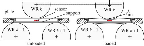
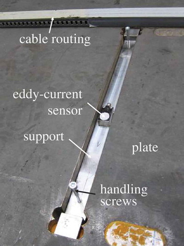
Figure 11. Support with mounted eddy-current sensor inserted into the test plate.

3.1. Experiment design

The first point is addressed by using a simple test plate at room temperature. As the cold plate is rather stiff, great forces can be exerted by only imposing small elastic deformations on the plate. It is assumed that the force–deflection relation of the test plate can be modelled by means of the linear load model presented in Section 2.8.

A method of dealing with the second point is illustrated in the Figures 10–13. In order to measure the deflection, the plate has longitudinal cut-outs that cover the distance of two neighbouring lower work rolls. In the cut-out, a support is placed that rests just on the lower work rolls. An ample clearance between the plate and the support ensures the plate does not apply any forces to the support, which is thus neither deformed nor displaced when the plate is loaded. An eddy-current distance sensor is mounted on the support. It directly measures the displacement of the upper roll k relative to the straight connection of the work rolls k − 1 and k + 1. This way, the work roll deflection in terms of the roll intermesh $v_{\mathrm{i}\mathrm{m}}^k,$ cf. Equation (28), is directly measured with a precision of 0.01 mm. Figure 11 shows a support inserted into a cut-out of the test plate.

During the experiments, the work rolls are not driven, that is, the test plate rests on the rolls. Consequently, dynamic effects on the deflection cannot be investigated with the proposed experiment. For instance, friction and lubricant conditions may vary while the plate is moved through the leveller. These effects can lead to changes in the force–deflection relations of contacts and in the distribution of forces between the parts of the leveller. However, effects in contacts between parts are expected to be small: in Section 2.6, it was shown that the posts, the screws and the subframes dominate the deflection of the machine.

In order to achieve load distributions of different widths, two test plates – a wide and a narrow one – were manufactured. The configuration of the wide plate is illustrated in Figure 12. The number of the sensors and their distribution over the plate is a trade-off between cost, machining complexity and desired spatial resolution. In this work, the roll intermesh of the work rolls 2 and 6 was measured equally distributed over the plate width at five locations $z_{\mathrm{o}\mathrm{u}\mathrm{t}}^l$, $z_{\mathrm{m}\mathrm{i}\mathrm{d}}^l$, $z_{\mathrm{c}\mathrm{t}\mathrm{r}}$, $z_{\mathrm{m}\mathrm{i}\mathrm{d}}^r$ and $z_{\mathrm{o}\mathrm{u}\mathrm{t}}^r$. 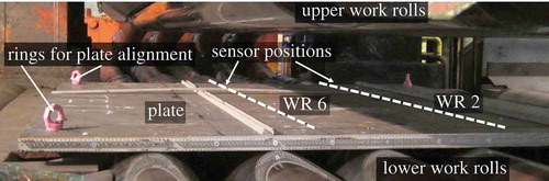A photograph of the wide test plate in the fully opened leveller is shown in Figure 13. The plate rests on the lower work rolls, while the roll 9 is at the leftmost part of the picture. The rings in the plate corners were used to manually align the plate.

Figure 12. Wide test plate with the sensor placements relative to the work and support roll locations.

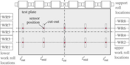
Figure 13. The wide test plate aligned in the considered leveller.

Before the experiments, the leveller was calibrated with F_tot = 1.18 MN. Different load cases were considered by varying the mean adjustment Δd_adc,mean, the tilt adjustment Δd_adc,tilt and the bending Δd_bend. The values for tilting and bending were preset while the upper frame was unloaded. Then, the upper frame was descended stepwise onto the test plate by increasing the mean adjustment. Each new set point was held constant for a while to wait for the decay of transients. Hence, only steady-state values are used for all the following analyses.

For the symmetrical model, the total load or levelling force F_tot of the leveller can be obtained from the screw forces ${\breve{F}}_{\mathrm{S}\mathrm{c}}$ by

(36) $F_{\mathrm{t}\mathrm{o}\mathrm{t}}=2\left({\breve{F}}_{\mathrm{S}\mathrm{c},\mathrm{e}\mathrm{n}}+{\breve{F}}_{\mathrm{S}\mathrm{c},\mathrm{e}\mathrm{x}}\right).$(36)

The measured total load force F_tot is derived as the sum of the four adjustment cylinder forces computed from the measured hydraulic pressure values. Corrections are made for the weight of the upper frame.

3.2. Validation results

Figure 14(a) and (b) shows the measured roll intermesh v_im,meas of four selected sensors plotted versus the corresponding mean adjustment Δd_adc,mean and the measured total load force F_tot, respectively, for an experiment where all upper support rolls are adjusted equally, that is, Δd_adc,tilt = Δd_bend = 0. Here, an offset correction was added to all roll intermesh signals so that they are zero when Δd_adc,mean is zero.

The roll intermesh is defined with respect to the undeformed and unloaded plate, cf. Equation (28). Practically, the origin of the reference coordinate system Ox⁰y⁰z is difficult to identify. Due to unknown manufacturing and assembling errors of the plate, the supports and the sensors, the origin cannot be calculated from nominal dimensions. Moreover, neither the origin nor the point of first contact can be precisely identified from the shown roll intermesh signals, as can be inferred from Figure 14(a). However, for Δd_adc,mean > 1.4 mm, the relation is approximately linear, indicating that the work rolls have established full contact with the plate. Moreover, the rolls seem to touch the plate not at the same instant, which indicates that the test plate is not exactly flat and thus exhibits a nonlinear force–deflection relation. This is also proven by the force–deflection diagram in Figure 14(b). Here, additionally, the computed ideal linear force–deflection relation of the test plate is shown for the special case of a uniform roll intermesh of all rolls, assuming nominal parameters. To allow for better comparison, this ideal curve is aligned at the maximum value of the deflection of the work roll 6 at z = z_ctr. Apparently, for high loads, the test plate behaves like the ideal characteristic, but it is more compliant for lower forces. This supports the hypotheses of non-ideal contact conditions due to flatness defects of the test plate.

Figure 14. Measured roll intermesh for selected rolls over the mean adjustment and the measured total load force for the large test plate.

The observations made earlier lead to the following consequences for the subsequent analysis: for the wide test plate, the leveller was recalibrated at F_tot = 6 MN, defining the origin of a new coordinate system ${\check{d}}_{\mathrm{a}\mathrm{d}\mathrm{c}}$ for the adjustment variables and ${\check{v}}_{\mathrm{i}\mathrm{m}}$ for the roll intermesh. For the narrow test plate, a similar threshold value was found.

The linear plate model was fitted to the measured behaviour in the load range 6 MN < F_tot < 16 MN. Here, the plate stiffness K_b,pl was adapted. This parameter fitting problem can be solved separately from the deflection model, because the plate deflection was measured directly.

In order to validate the deflection model, roll intermeshes ${\check{v}}_{\mathrm{i}\mathrm{m}}$ for different load cases relative to the adjustment ${\check{d}}_{\mathrm{a}\mathrm{d}\mathrm{c},\mathrm{m}\mathrm{e}\mathrm{a}\mathrm{n}}={\check{d}}_{\mathrm{a}\mathrm{d}\mathrm{c},\mathrm{t}\mathrm{i}\mathrm{l}\mathrm{t}}={\check{d}}_{\mathrm{b}\mathrm{e}\mathrm{n}\mathrm{d}}=0\mathrm{m}\mathrm{m}$ were calculated and compared with the respective measured roll intermeshes ${\check{v}}_{\mathrm{i}\mathrm{m},\mathrm{m}\mathrm{e}\mathrm{a}\mathrm{s}}$. Only roll intermesh differences are compared, that is, the difference of two profiles of two different load cases. This way, the deflection state corresponding to the calibration point does not need to be known. Hence, for both the wide and the narrow plates, a case with only a small mean adjustment ${\check{d}}_{\mathrm{a}\mathrm{d}\mathrm{c},\mathrm{m}\mathrm{e}\mathrm{a}\mathrm{n}}$ was chosen as reference, and for the remainder of this section, roll intermesh results are given as difference $\mathrm{\Delta }{\check{v}}_{\mathrm{i}\mathrm{m}}$ to these reference cases. Table 1 lists the considered load cases. Moreover, a Coulomb friction part of the total load force of about ±0.12 MN was identified by comparing the steady-state forces before and after displacement in different directions.

Figure 15 shows the measured and computed roll intermesh differences $\mathrm{\Delta }{\check{v}}_{\mathrm{i}\mathrm{m}}$ for both test plates and for selected load cases. Obviously, the measured roll intermesh differences indicate that the problem is not exactly symmetrical. Nevertheless, in the mean, the model captures very well the expected characteristic of the deflection of the leveller, as can be inferred from the intermesh profiles in Figure 15. The cases ‘wide 1’ and ‘narrow 1’ with zero tilt and bending adjustment, cf. Figure 15(a) and (c), clearly show that the lateral centre of the machine deflects more than the border, resulting in a lower roll intermesh in the centre. Moreover, an inhomogeneous deflection in longitudinal direction may be inferred from all cases shown in Figure 15. The absolute roll intermesh at work roll 6 is lower than at work roll 2. The effect of bending and tilting becomes apparent in the cases ‘wide 4’ and ‘narrow 3’, where the absolute roll intermesh at the lateral machine centre (bending) and in total at the work roll 2 (tilting) are significantly increased.

Table 1. List of load cases.

Name	$\mathrm{\Delta }{\check{d}}_{\mathrm{a}\mathrm{d}\mathrm{c},\mathrm{m}\mathrm{e}\mathrm{a}\mathrm{n}}$ (mm)	$\mathrm{\Delta }{\check{d}}_{\mathrm{a}\mathrm{d}\mathrm{c},\mathrm{t}\mathrm{i}\mathrm{l}\mathrm{t}}$ (mm)	$\mathrm{\Delta }{\check{d}}_{\mathrm{b}\mathrm{e}\mathrm{n}\mathrm{d}}$ (mm)	ΔFtot (MN)
wide 1	0.71	−0.01	0.02	3.0
wide 2	1.29	−0.01	0.02	5.6
wide 3	0.45	−0.01	−0.59	2.6
wide 4	0.11	0.03	−1.17	2.5
narrow 1	1.24	−0.01	0.09	4.0
narrow 2	0.34	−1.15	−0.58	2.3
narrow 3	0.02	0.71	−0.61	1.3
narrow 4	0.41	0.02	−0.73	2.8

Figure 15. Comparison of measured and calculated roll intermesh difference.

Also in terms of the quantitative accuracy, the model shows very good performance. The residuals $\mathrm{\Delta }{\check{v}}_{\mathrm{i}\mathrm{m},\mathrm{m}\mathrm{e}\mathrm{a}\mathrm{s}}-\mathrm{\Delta }{\check{v}}_{\mathrm{i}\mathrm{m}}$ between measurement and model are shown in Figure 16. Here, $\mathrm{\Delta }{\check{v}}_{\mathrm{i}\mathrm{m},\mathrm{m}\mathrm{e}\mathrm{a}\mathrm{s}}$ is represented as the mean value of both sides for the off-centre sensor positions. The model only shows residuals up to 0.08 mm. This is quite small compared to the nominal adjustment. As an example, the case ‘narrow 1’ in Figure 15(c) is considered. With an almost vanishing tilt adjustment $\mathrm{\Delta }{\check{d}}_{\mathrm{a}\mathrm{d}\mathrm{c},\mathrm{t}\mathrm{i}\mathrm{l}\mathrm{t}}=-0.01\mathrm{m}\mathrm{m}$, the mean adjustment $\mathrm{\Delta }{\check{d}}_{\mathrm{a}\mathrm{d}\mathrm{c},\mathrm{m}\mathrm{e}\mathrm{a}\mathrm{n}}=1.24\mathrm{m}\mathrm{m}$ would lead to a roll intermesh of −1.24 mm at roll 6 for an ideally rigid leveller. For the real, compliant leveller, only a mean resulting roll intermesh of about −0.1 mm is both measured and calculated. Moreover, the calculated total levelling forces are very close to the measured forces.

Figure 16. Residuals of the model for the considered load cases of Table 1.

4. Conclusion

In this work, a mathematical deflection model of a hot leveller with bending mechanism was systematically developed. The model structure can be easily transferred to levellers with an arbitrary adjustment of the support rolls. Linear compliance models of the individual parts are derived by means of compression members, beams and – for the complex subframes – condensation of FE models. Contact nonlinearities for small forces are approximately modelled as backlash.

A new principle for the measurement of the deflection of a leveller was presented and successfully applied for the validation of the model. The deflection of the work rolls is measured by means of displacement sensors that are inserted in cut-outs of test plates. The supports of the sensors stay unloaded and thus undeformed during the experiments. The test plates are modelled by means of linear elastic stripes. However, it was observed that the plates used in the validation experiments exhibit a significant nonlinear elastic force–deflection behaviour. Furthermore, the point of first contact between work rolls and the plate is highly uncertain. Both points have to be addressed in future experiments in order to validate the full nonlinear deflection model including backlash.

Nevertheless, the direct measurement of the plate deformation allowed for the validation of the linear part of the deflection model. The model shows a very good accordance with the measured roll intermesh, where the accuracy of the roll intermesh prediction is better than 0.08 mm.

The validated deflection model can be used in the first place to analyse the influence of the deflection on the resulting plate flatness both in lateral and longitudinal direction of the product. Furthermore, it can be applied to optimally compensate for the deflection. Because the loads of critical parts like the support rolls are an inherent part of the solution of the deflection problem, they can be monitored and constrained in order to prevent premature failure due to overloading.

Additional information

Funding

The second author gratefully acknowledges financial support provided by the Austrian Academy of Sciences in the form of an APART-fellowship at the Automation and Control Institute of Vienna University of Technology.

Notes

1. Henceforth, all quantities related to the subframes are indicated by the subscript F.

Appendix A. Kinematics of the nominal roll adjustment

The adjustment variables $d_{\mathrm{a}\mathrm{d}\mathrm{c},\mathrm{e}\mathrm{n}},$ $d_{\mathrm{a}\mathrm{d}\mathrm{c},\mathrm{e}\mathrm{x}},$ ${\phi }_{\mathrm{b}\mathrm{e}\mathrm{n}\mathrm{d}},$ $d_{\mathrm{a}\mathrm{d}\mathrm{r},\mathrm{e}\mathrm{n}}$ and $d_{\mathrm{a}\mathrm{d}\mathrm{r},\mathrm{e}\mathrm{x}}$ define the nominal vertical adjustment $a{d}_{\mathrm{S}\mathrm{R}}\left(z\right)$of the support roll centres in terms of pure rigid body displacements. The strokes $d_{\mathrm{a}\mathrm{d}\mathrm{c},\mathrm{e}\mathrm{n}}$ and $d_{\mathrm{a}\mathrm{d}\mathrm{c},\mathrm{e}\mathrm{x}}$ of the adjustment cylinders can be equally written as mean value

(A1a) $d_{\mathrm{a}\mathrm{d}\mathrm{c},\mathrm{m}\mathrm{e}\mathrm{a}\mathrm{n}}=\frac{1}{2}\left(d_{\mathrm{a}\mathrm{d}\mathrm{c},\mathrm{e}\mathrm{n}}+d_{\mathrm{a}\mathrm{d}\mathrm{c},\mathrm{e}\mathrm{x}}\right)$(A1a)

and difference value

(A1b) $d_{\mathrm{a}\mathrm{d}\mathrm{c},\mathrm{t}\mathrm{i}\mathrm{l}\mathrm{t}}=d_{\mathrm{a}\mathrm{d}\mathrm{c},\mathrm{e}\mathrm{n}}-d_{\mathrm{a}\mathrm{d}\mathrm{c},\mathrm{e}\mathrm{x}}.$(A1b)

The horizontal location of the adjustment cylinders in the coordinate system $O{x}^0{y}^{0}z$ is described by the coordinates $\pm x_{\mathrm{S}\mathrm{c},\mathrm{e}\mathrm{x}}$ and $z_{\mathrm{S}\mathrm{c}},$ see Figure 7. The adjustment cylinders displace the support rolls of the upper work roll, $k\in \left\{2,4,6,8\right\},$ with respect to the coordinate $y^{\mathrm{u}\mathrm{p}}$ by

(A2) $a{d}_{\mathrm{a}\mathrm{d}\mathrm{c}}^k=-d_{\mathrm{a}\mathrm{d}\mathrm{c},\mathrm{m}\mathrm{e}\mathrm{a}\mathrm{n}}+\frac{d_{\mathrm{a}\mathrm{d}\mathrm{c},\mathrm{t}\mathrm{i}\mathrm{l}\mathrm{t}}}{2x_{\mathrm{S}\mathrm{c},\mathrm{e}\mathrm{x}}}{x}_{\mathrm{W}\mathrm{R}}^k.$(A2)

Here, $x_{\mathrm{W}\mathrm{R}}^k$ refers to the longitudinal position of work roll k in the coordinate system $O{x}^0{y}^{0}z$, cf. Figure 2. At the lateral coordinate z, the bending adjustment leads to the vertical displacement

(A3) $a{d}_{\mathrm{b}\mathrm{e}\mathrm{n}\mathrm{d}}\left(z\right)=\frac{-{\phi }_{\mathrm{b}\mathrm{e}\mathrm{n}\mathrm{d}}}{2}\left(z-z_{\mathrm{S}\mathrm{c}}\right),$(A3)

which is the same for all upper support rolls. Sometimes, the bending adjustment is given in terms of the nominal adjustment $d_{\mathrm{b}\mathrm{e}\mathrm{n}\mathrm{d}}$ of the centre of the upper subframe, that is,

(A4) $d_{\mathrm{b}\mathrm{e}\mathrm{n}\mathrm{d}}=\frac{{\phi }_{\mathrm{b}\mathrm{e}\mathrm{n}\mathrm{d}}}{2}{z}_{\mathrm{S}\mathrm{c}}.$(A4)

Equations (A2) and (A3) are superposed to get the total nominal vertical adjustment of a point on a support roll of the upper subframe

(A5) $a{d}_{\mathrm{S}\mathrm{R}}^k\left(z\right)=a{d}_{\mathrm{a}\mathrm{d}\mathrm{c}}^k+a{d}_{\mathrm{b}\mathrm{e}\mathrm{n}\mathrm{d}}\left(z\right),k\in \left\{2,4,6,8\right\}.$(A5)

The lower work rolls $k\in \left\{2,4,6,8\right\}$ are not adjustable. The laterally uniform adjustment of the entry and exit roll with respect to $y^{\mathrm{l}\mathrm{o}}$ is defined by, cf. Figure 1,

(A6) $a{d}_{\mathrm{S}\mathrm{R}}^1=-d_{\mathrm{a}\mathrm{d}\mathrm{r},\mathrm{e}\mathrm{n}}\mathrm{a}\mathrm{n}\mathrm{d}a{d}_{\mathrm{S}\mathrm{R}}^9=-d_{\mathrm{a}\mathrm{d}\mathrm{r},\mathrm{e}\mathrm{x}}.$(A6)

References

- V.B. Ginzburg, High-Quality Steel Rolling: Theory and Practice, Manufacturing engineering and materials processing, Marcel Dekker, Inc., New York, 1993.
- E. Doege, R. Menz, and S. Huinink, Analysis of the levelling process based upon an analytic forming model, CIRP Ann. Manufacturing Technol. 51 (2002), pp. 191–194. doi:10.1016/S0007-8506(07)61497-8.
- L.S. Henrich, Theoretische und experimentelle Untersuchungen zum Richtwalzen von Blechen, Ph.D. diss., Fachbereich Maschinentechnik, Universität-Gesamthochschule Siegen, 1993.
- B.A. Behrens, T. El Nadi, and R. Krimm, Development of an analytical 3D-simulation model of the levelling process, J. Mater. Process. Technol. 211 (2011), pp. 1060–1068. doi:10.1016/j.jmatprotec.2011.01.007.
- J. Mischke and J. Jońca, Simulation of the roller straightening process, J. Mater. Process. Technol. 34 (1992), pp. 265–272. doi:10.1016/0924-0136(92)90116-A.
- L. Bodini, O. Ehrich, and M. Krauhausen, Heavy plate leveler improvement by coupling a model to a flatness gauge, in Proceedings of the 3rd International Steel Conference on New Developments in Metallurgical Process Technologies, Düsseldorf, Germany, 2007, pp. 246–251.
- S. Krämer, R. Dehmel, G. Horn, T. Koch, J. Lemke, and P. Lixfeld, Plate production using most modern process models, in Proceedings of the 4th International Conference on Modelling and Simulation of Metallurgical Processes in Steelmaking, STEELSIM, METEC InSteelCon 2011, Düsseldorf, 2011.
- T. Aoyama, The latest technology of the heavy plate leveler, AIS Tech 2011, Indianapolis, 2011, p. 9.
- DIN 55189-1, Machine tools, determination of the ratings of presses for sheet metal working under static load, Part 1: Mechanical presses, (in German), DIN Deutsches Institut für Normung e.V., Berlin, 1988.
- T. Koenig, A. Steinboeck, F. Schausberger, A. Kugi, M. Jochum, and T. Kiefer, Online calibration of a mathematical model for the deflection of a rolling mill, in Proceedings of the 9th International and 6th European Rolling Conference, Venice, 2013.
- F.A. Batty and K. Lawson, Heavy plate levellers, J. Iron Steel Inst. 203 (1965), pp. 1115–1128.
- M. Baumgart, A. Steinboeck, A. Kugi, B. Douanne, G. Raffin-Peyloz, L. Irastorza, and T. Kiefer, Modeling and active compensation of the compliance of a hot leveler, Steel Res. Int., Special Edition ICTP2011 (2011), pp. 337–342.
- M. Baumgart, A. Steinboeck, A. Kugi, G. Raffin-Peyloz, L. Irastorza, and T. Kiefer, Optimal active deflection compensation of a hot leveler, in Preprints of the IFAC Workshop on Automation in the Mining, Mineral and Metal Industries, Gifu, 2012, pp. 30–35.
- M. Baumgart, A. Steinboeck, A. Kugi, G. Raffin-Peyloz, B. Douanne, L. Irastorza, and T. Kiefer, Active compliance compensation of a hot leveler, in Proceedings of the 4th International Conference on Modelling and Simulation of Metallurgical Processes in Steelmaking, STEELSIM, METEC InSteelCon 2011, Düsseldorf, 2011, pp. 1–10.
- W.C. Young and R.G. Budynas, Roark’s Formulas for Stress and Strain, 7th ed., McGraw-Hill, New York, NY, 2002.
- E. Doege and B.A. Behrens (eds.), Handbuch Umformtechnik, 2nd ed., Springer, Berlin, 2010.
- G. Beer and J. Watson, Introduction to Finite and Boundary Element Methods for Engineers, John Wiley & Sons, Chichester, 1992.
- C. Felippa, K. Park, and M.J. Filho, The construction of free-free flexibility matrices as generalized stiffness inverses, Comput. Struct. 68 (1998), pp. 411–418. doi:10.1016/S0045-7949(98)00068-6.
- H. Becker, W. Guericke, R. Hinkfoth, and B. König, Walzwerke: Maschinen und Anlagen, 1st ed., VEB Deutscher Verlag für Grundstoffindustrie, Leipzig, 1981.
- VDI Guideline 2230, Systematic Calculation of High Duty Bolted Joints – Joints with One Cylindrical Bolt, Verein Deutscher Ingenieure, Düsseldorf, 2003.
- F. Hibino, The practical formula for leveling strain in a roller leveler, J. Japan Soc. Technol. Plasticity. 31 (1990), pp. 208–212.
- J. Kierzenka and L. Shampine, A BVP solver based on residual control and the MALTAB PSE, ACM Trans. Math. Software. 27 (2001), pp. 299–316. doi:10.1145/502800.502801.