A dynamic modelling framework for control-based computing system design

Abstract

This manuscript proposes a novel viewpoint on computing systems’ modelling. The classical approach is to consider fully functional systems and model them, aiming at closing some external loops to optimize their behaviour. On the contrary, we only model strictly physical phenomena, and realize the rest of the system as a set of controllers. Such an approach permits rigorous assessment of the obtained behaviour in mathematical terms, which is hardly possible with the heuristic design techniques, that were mainly adopted to date. The proposed approach is shown at work with three relevant case studies, so that a significant generality can be inferred from it.

Keywords:

• computing systems
• feedback control
• scheduling
• memory management
• resource allocation

1. Introduction

The complexity of many computing system functionalities is nowadays abruptly increasing [1]. For example, consider the Linux scheduler. In the Kernel version 2.4.37.10 (September 2010), all of its code was contained in a single file of 1397 lines. In version 2.6.39.4 (August 2011), the scheduler code is spread among 13 files for a total of 17,598 lines.

Indeed, when such ‘explosions’ are experienced, the overall design approach to the functionalities is to be somehow reconsidered. The presented research proposes to adopt a design approach, entirely based on the systems and control theory. This would allow the reduction of heuristics that are widely present in modern operating (and computing) systems. The main advantage of the abolition of heuristics is that the properties of interest could then be formally assessed [2]. If a control-theoretical design is carried out, the formal tools of stability, observability, reachability and so forth can be brought into play, to state that the system will behave as expected in the presence of unpredictable situations and disturbances. It is worth noticing that to the best of our knowledge this approach has not yet been attempted, that is, no computing system functionality has to date been conceived and developed based on a dynamic model of some physical phenomenon to be controlled.¹

The lack of a system- and control-theoretical attitude in the design of computing system components has quite clear historical reasons, see again [2]. For the purpose of this paper, one fact is most important to notice in this respect. While in any other context controlled objects can be modelled based on physical (first) principles, this is not the case for computing systems, because in such systems the ‘physics’ is created by the designer him/herself. This is well exemplified by a famous quote by Linus Torvalds [3], who wrote

I’m personally convinced that computer science has a lot in common with physics. Both are about how the world works at a rather fundamental level. The difference, of course, is that while in physics you’re supposed to figure out how the world is made up, in computer science you create the world. Within the confines of the computer, you’re the creator. You get to ultimately control everything that happens. If you’re good enough, you can be God. On a small scale.

In the absence of a modelling framework, however, system design (or according to Linus, creation) is invariantly carried out directly in an algorithmic setting, without any means to formally assess its behaviour. As ‘more physics’ is created, the absence of a rigorous dynamic description may thus, sooner or later, pose intractable problems as for its governance: the scheduler explosion just mentioned is a notable example of this trend.

As a consequence, the non-system-theoretical scenario sketched out above could to date be tolerated, but it cannot be assured that said tolerability will carry over to the future. Rigorous – and possibly simple – modelling frameworks to ground system design upon are becoming a necessity, since there is much to do in this direction before problems exacerbate [4].

The main message this paper wants to convey is that if one accepts to redesign part of said system – that has been conceived in an algorithmic way – such a framework can be found by (usefully) limiting the model scope to describe the real physical phenomenon on which the addressed aspects of the system behaviour depend. If this is done, surprisingly simple formalisms can be used – a noticeable example indeed of process/control co-design, and in the authors’ opinion, a step forward with respect to previous research.

This paper concentrates on the modelling side of the problem, by showing the ideas above at work, extending [5] with an additional and deeper analysis of the examples treated therein, and proposing a novel framework dealing with memory management. Some words are spent on the consequent advantages in terms of system (and control) design, limiting however the depth to sketching out possible solutions, and referring the interested reader to the convenient literature when this is applicable. On a similar front, a comprehensive presentation of the current state of this research, specialized however to the context of operating systems, can be found in [2].

In this paper, the formalism of discrete-time dynamic systems is exploited. An alternative – and in some cases also coordinated – approach for the control of computing system could be based on supervisory control and discrete event systems [6,7]. However, in the authors’ opinion, the modelling effort carried out in this paper would greatly simplify the design of the controllers also if supervisory control was the control paradigm of choice, since it provides with more insights in the problem to be solved and in what influences the dynamics to be controlled.

2. The quest for physics

Before going into details, in this section we spend some words to show that many typical problems in the computing system domain can be addressed with a general viewpoint by adopting a dynamic modelling framework. In the next sections, the ideas presented below in general, are specialized and declined in some representative examples.

At the very core of any computing system behaviour, there is some strictly physical phenomenon. For example, in the case of an operating system scheduler, that phenomenon has the form

$\mathrm{a}\mathrm{c}\mathrm{c}\mathrm{C}\mathrm{P}\mathrm{U}\left(k\right)=\mathrm{a}\mathrm{c}\mathrm{c}\mathrm{C}\mathrm{P}\mathrm{U}\left(k-1\right)+\mathrm{b}\mathrm{u}\mathrm{r}\mathrm{s}\mathrm{t}\left(k\right)+\mathrm{d}\mathrm{i}\mathrm{s}\mathrm{t}\mathrm{u}\mathrm{r}\mathrm{b}\mathrm{a}\mathrm{n}\mathrm{c}\mathrm{e}\left(k\right)$

where k counts discrete-time instants, $\mathrm{a}\mathrm{c}\mathrm{c}\mathrm{C}\mathrm{P}\mathrm{U}\left(\cdot \right)$ is the CPU time accumulated by a task, $\mathrm{b}\mathrm{u}\mathrm{r}\mathrm{s}\mathrm{t}\left(\cdot \right)$ is the CPU time slice allotted to the task and $\mathrm{d}\mathrm{i}\mathrm{s}\mathrm{t}\mathrm{u}\mathrm{r}\mathrm{b}\mathrm{a}\mathrm{n}\mathrm{c}\mathrm{e}\left(\cdot \right)$ accounts for any difference between $\mathrm{b}\mathrm{u}\mathrm{r}\mathrm{s}\mathrm{t}\left(\cdot \right)$ and the actual CPU use by the task.

Similar models can be obtained for many other problems. For example, suppose that an application needs to accomplish its task at a specified rate, like a video encoder that needs to process a desired number of frames per second. Suppose that the application speed depends on some resources, like the number of processing units, and these resources are shared with other applications, so that some arbitration mechanism is required to manage them. In such a case, the present state of the application’s progress towards its goal depends on the progress state before the last resource arbitration instant and on the allotted resources at that instant.

In the most general case, the behaviour of a computing system ultimately depends on extremely fine-grained facts, down to the detailed behaviour of any single assembler instruction and electronics transient. This is one of the main differences between modelling computing systems or purely physical objects. The fine-grained physical level is often the only level that can be rigorously defined in computing system modelling.

On the contrary, in physical systems, there is usually a more abstract modelling level. In thermal systems, for example, one can avoid treating fine-grain phenomena (in that case, molecular motions) since there exist suitable macro-physic entities (e.g., temperature or enthalpy) that allow to write rigorous balances (e.g., of energy) to base dynamic models upon.

In the development of computing systems, in addition, no set of ‘first principles’ has de facto ever been sought. Sticking again to the scheduling example, action policies are typically defined as ‘give the CPU to the task with the earliest deadline’ by foreseeing their effect in some nominal conditions (for a schedulable task pool, doing so there will be no misses). Alternatively, in the control of the application’s progress, the action policy can be expressed as ‘give an additional core if the application is too slow, remove a core if the application is too fast’. Apparently, the algorithmic attitude to the problem hinders the possibility to formally address dynamic properties of the system at hand, as it attempts to find a (control) solution without a modelling phase.

In the addressed domain, in other words, there is classically no distinction among the behaviour of the system in the absence of such actions, the desired behaviour of the same system and the way actions are to be determined based on the above. There is no evidence of the fundamental elements of a (control-oriented) modelling process.

Deepening the analysis, one may object that many works deal with computing system control, and do use control-theoretical methodologies, see, for example, [8–11] and, particularly, [12]. This is true, but virtually all of them take the computing system as is and close loops around it (e.g., aiming at a certain Central Processing Unit (CPU) distribution by altering task deadlines). Doing so however requires to model the core phenomenon plus all the ‘created physics’ around it (e.g., the existing deadline-based scheduler).

In the authors’ opinion, the presence of such ‘unconsciously created’ physics is a major reason for the complexity of most computing systems’ models, at least as far as the ultimate scope of said models is to design parts of those systems in the form of controllers. To circumvent the problem, one should thus in the first place evidence the core phenomenon, that is, that part of the system behaviour that really relies on physics and cannot be altered. Most often, modelling that phenomenon is enough to describe the system in a view to suitably control it [5,13]. In some cases, in addition, the so obtained models will be natively (almost) uncertainty free, making control design and assessment very straightforward. In other cases, there may be relevant uncertainty, or – in other words – some aspects of the system behaviour will not admit a clear physical interpretation. In such cases, the advice is to figure out some convenient grey box description – as opposite to the black box approaches that the literature dominantly presents [10,12] – based on qualitative considerations on input–output relationships. As will be shown, this approach generally leads to more complex but still tractable models: control design may be correspondingly harder, but still there will be the possibility of a rigorous assessment.

In the following section, some examples are shown of how the proposed approach leads to dynamic models of computing system components that can successfully serve the evidenced needs, while being very simple and thus suitable for powerful and rigorous analysis and control result assessment.

3. A unified framework for task scheduling

This section shows how the task scheduling in a pre-emptive single-processor system can be fully treated having as model class that of discrete-time dynamic systems, in some cases even linear and time invariant. A few words are also spent on the natural attitude of said modelling formalisms to scale up towards, for example, multicore or multiprocessor contexts, where any other modelling formalism and design approach do experience severe difficulties. The reader interested in more details on the problems encountered by literature approaches can refer, for example, to [14].

Consider a single-processor multitasking system with a pre-emptive scheduler, pre-emptive meaning that the scheduler can interrupt the current task and substitute it with another one. Let N be the number of tasks to schedule. Define the round as the time between two subsequent scheduler interventions. Let the column vectors ${\tau }_p\left(k\right)\in R^N$, ${\tau }_r\left(k\right)\in R$, ${\rho }_p\left(k\right)\in R^N$, $b\left(k\right)\in R^{n\left(k\right)}$ and $\delta b\left(k\right)\in R^{n\left(k\right)}$, $1\le n\left(k\right)\le N\mathrm{\forall }k$ represent, respectively,

• the CPU times actually allocated to the tasks in the kth round,

• the time duration of the kth round,

• the times to completion (i.e., the remaining CPU time needed by the task to end its job) at the beginning of the kth round for the tasks that have a duration assigned (elements corresponding to tasks without an assigned duration will be $+\mathrm{\infty }$, therefore allowing for the presence of both batch and interactive tasks),

• the bursts, that is, the CPU times allotted by the scheduler to the tasks at the beginning of the k-th round,

• the disturbances possibly acting on the scheduling action during the kth round (e.g., because one of the tasks release the CPU before its burst has expired or because of an interrupt management amidst the task operation),

where n(k) is the number of tasks that the scheduler considers at each round. In the traditional scheduling policies, n(k) is constant and equal to one – an example of aprioristic constraint that in principle can be relaxed, maybe resulting in better performances. Denote by t, the total time actually elapsed from the system initialization.

A very simple model for the phenomenon of interest is then

(1) $\left\{\begin{array}{c}{\tau }_p\left(k\right)=S_{\sigma }b\left(k-1\right)+\delta b\left(k-1\right)\\ {\tau }_r\left(k\right)=1_{1\times N}{\tau }_p\left(k-1\right)\\ {\rho }_p\left(k\right)=max\left({\rho }_p\left(k-1\right)-S_{\sigma }b\left(k-1\right)-\delta b\left(k-1\right),0\right)\\ t\left(k\right)=t\left(k-1\right)+{\tau }_r\left(k\right)\end{array}\right)$(1)

where $1_{1\times N}$ is a row vector of length N with unit elements, and $S_{\sigma }\in \mathrm{\Sigma }$ a $N\times n\left(k\right)$ switching matrix. The elements of $S_{\sigma }$ are zero or one, and each column contains at most one element equal to one. Matrix $S_{\sigma }$ determines which tasks are considered in each round, to the advantage of generality (and possibly for multiprocessor extensions). Notice that, since n(k) is bounded, the set $\mathrm{\Sigma }$ is finite for any N.

Several scheduling policies can be described with the presented formalism, by merely choosing n(k) and/or $S_{\sigma }\left(k\right)$. For example

• n = 1 and a N-periodic $S_{\sigma }$ with

  (2) $S_{\sigma }\left(k\right)\ne S_{\sigma }\left(k-1\right),2\le k\le N$(2)

  produce all the possible Round Robin (RR) policies having the (scalar) b(k) as the only control input, and obviously the pure RR if b(k) is kept constant,

• generalizations of the RR policy are obtained if the period of $S_{\sigma }$ is greater than N, and Equation (2) is obviously released,

• n = 1 and a $S_{\sigma }$ chosen so as to assign the CPU to the task with the minimum row index and a ${\rho }_p$ greater than zero produces the First Come First Served (FCFS) policy,

• n = 1 and a $S_{\sigma }$ that switches according to the increasing order of the initial ${\rho }_p$ vector produces the Shortest Job First (SJF) policy (notice that this is the same as SRTF if no change to the task pool occurs, as can be seen in Figure 1),

• n = 1 and a $S_{\sigma }$ selecting the task with the minimum ${\rho }_p$ yields the Shortest Remaining Time First (SRTF) policy.

The capability of model (1) to reproduce the mentioned policies is shown in Figure 1, in the case of n(k) = 1, N = 5 and $S_{\sigma }\left(k\right)$ chosen as described above.

Figure 1. Capability of the presented single model of reproducing classical scheduling policies such as RR, FCFS, SJF and SRTF.

In all these policies, the core phenomenon can be noticed in the form

${\tau }_p\left(k\right)=S_{\sigma }b\left(k-1\right)+\delta b\left(k-1\right).$

Also the ‘added physics’ can be noticed, as the algorithm used to select n(k) and/or $S_{\sigma }\left(k\right)$.

If one attempts to model both things together, to close the loop around the existing scheduler, then switching systems must be brought into play.

If, on the contrary, one models the core phenomenon only, and treats all the rest as part of the controller, the single and trivial equation just written is enough. Notice that here in modelling the core phenomenon no uncertainty is present, nor is there any measurement error, since the only required operation is to read the system time.

Based on model (1) one can thus abandon ‘non control theoretical’ (and often not even closed-loop) choices of S_σ as in the examples just sketched, and synthesize schedulers as controllers with very simple blocks, for example, of the proportional integral or Model Predictive Control (MPC) type [15,16]. The so conceived policies are tendentiously less computational intensive than those where a control loop is conversely closed around an already functional scheduler, that is, not around the core phenomenon only.

For example, some works introduce controllers to adjust the bursts, with the purpose of keeping the entire system utilization below a specified upper bound [17–19]. In these works, the burst duration is adjusted according to the results of the execution of a controller, built to optimize different cost functions. Each of these cost functions requires to redesign the control strategy, and no control-based selection of the next task is envisioned. On a different page, the authors of [20] reorder the list of tasks to be scheduled with a RR algorithm in an embedded device, with the aim of reducing cache misses. Control is introduced to meet a system requirement by acting on a parameter of a fully functional scheduler, rather than to simplify the design of the entire scheduler.

The approach proposed here, instead, models the core phenomenon and uses that model to pursue a real control theoretical solution, where properties of the closed-loop system could be formally proved. In this respect, a possibility is to endow (Equation (1)) with a cascade control structure, aimed at controlling both ${\tau }_r$, that is, the round duration, and the distribution of said duration among the active tasks. This can be done with very simple controllers, as shown in [15], and allows to specify the desired behaviour as a certain level of responsiveness (corresponding to a round duration setpoint) and fairness (related to the mentioned distribution). The paper just quoted also contains comparisons with some major (non-control-centric) scheduling policies, witnessing the advantages of the proposed approach. Note that the said approach allows to give a control-theoretical sense to terms like ‘responsiveness’ and ‘fairness’, that are widely used and well understood in the computing system community.

4. A unified framework for memory management

In this section, the proposed approach is applied to another core functionality of operating systems, namely that of memory management.

The operation of a memory manager works can be (roughly) described as follows. The Random Access Memory (RAM) in a computing system is divided in pages of fixed size. Those pages can be allocated to processes running in the operating system, which make memory requests. Of course, the quantity of available memory is limited by the total amount of RAM, and situations in which the processes are requiring more than the said upper bound may occur. The memory manager needs to be able to handle such cases, by temporarily saving some pages on disk, that is, by ‘swapping’ out pages through a specified policy, most frequently the so called ‘Least Recently Used’ (LRU). Those swapped pages can be requested in a different moment by an application (such an event being termed a ‘page fault’), and the memory manager is in charge of retrieving the appropriate pages and swap them back in RAM.

The relevance of the problem stems from several reasons. Even if the advances of technology make much more memory available for running applications, these are steadily more demanding in terms of memory pages. Memory is thus still a limited, thus critical, resource. Furthermore, memory is continuously requested and relinquished by processes over time, in an a priori hardly predictable manner; as such, the time scale of memory usage – thus management – is quite fast.

The LRU-based ‘traditional’ attitude towards memory management, sketched out above and dating back to works like [21–23], has two major issues. One is related to the system-wide nature of the LRU scheme, the other to the purely demand-based (or in other terms, event-triggered) activation of the memory manager. As a result, its behaviour is not optimal in many significant use cases.

A typical example is when a memory-intensive background task is run concurrently with some interactive ones, which can easily happen, for example, when using the same machine for running both heavy batch jobs and a window manager to provide a graphical user interface. When the background task’s memory allocations cause the exhaustion of the available RAM, the LRU scheme will swap out pages from arbitrary processes, most probably including the interactive ones, thus causing a significant reduction in their responsiveness. This is caused by the lack of a memory manager that can act on a per-process basis, so as to control which are the processes that have exceeded their memory limit, and have to be selected as targets for swap-outs.

The negative impact of swapping out pages onto application responsiveness is a widely known fact; however at present (at least, to the best of the authors’ knowledge) no systematic attempts to model the problem have emerged, and only ad hoc algorithmic solutions have been introduced.

Another limitation of current memory management systems, as mentioned, is their purely event-triggered nature. A typical example that exacerbates this limitation is when a process transiently allocates a large amount of memory, as it frequently happens for the linking phase at the end of the compilation of large software projects. In this case, part of that process will be swapped out and, due to the system-wide LRU scheme, part of other processes also most likely will. When the complex task ends, the memory occupation drops sharply, resulting in a large amount of free RAM. If in this situation the system is left idle, it will not recover responsiveness as fast as it could, due to swap-in being only triggered by application page faults. Therefore, it may happen that memory pages remain swapped out for a long time even if RAM is available. Subsequently, when a process requests those pages, a disk access will be triggered, stalling the process and decreasing its responsiveness. Moreover, the swap-in of those pages may occur when the CPU is highly loaded, while from the swap-out instant till the page faults there may have been plenty of time with a low CPU load.

Summarizing, there are two fundamental questions that current memory management schemes fail to address, which are what to swap and when to do it. The first question addresses per-process memory limits, and could be used to achieve memory access temporal isolation [24]. The second question opens the door to transfers between swap and RAM that are time triggered instead of event triggered by process page faults. In the opinion of the authors, this is another problem for which hardly any modelling effort has been spent to date, having as result a practically ubiquitous use of pure heuristics, and thus a management (i.e., control) that falls significantly short of perfection. When control-based techniques were applied by closing loops around a memory manager conceived in the traditional way rather than around the core phenomenon alone, the same attitude has often given rise to quite complex solutions, see, for example, [25].

Analysing the situation with the proposed approach, on the contrary, it is quite straightforward to state memory management as a feedback control problem, by posing for it the following objectives:

1. use as much RAM as possible without saturating,

2. give each process a (soft) quota to make it a candidate for swap-outs when this is exceeded (not forbidding anyway its allocation, whence the ‘soft’ adjective above), and

3. un-swap memory back to RAM when this is possible, based on a time-, not only event-triggered mechanism.

Adopting this viewpoint, here too the core phenomenon physics is quite simple, as the generic (ith) process can be represented by the discrete-time, linear and time-invariant model

(3) $\left\{\begin{array}{c}{m}_i\left(k\right)=m_i\left(k-1\right)+a_i\left(k-1\right)-d{m}_i\left(k-1\right)+p{f}_i\left(k-1\right)+u_i\left(k\right)\\ s_i\left(k\right)=s_i\left(k-1\right)-d{s}_i\left(k-1\right)-p{f}_i\left(k-1\right)-u_i\left(k-1\right)\end{array}\right)$(3)

where the state variables m_i and s_i are respectively the quantity of allocated RAM and swap memory. The index k counts the memory-affecting operations, making Equation (3) discrete-time but not sampled-signals. The other quantities are either process-generated requests – that is, a_i, dm_i, pf_i, ds_i, treated here as disturbances – or memory-manager decisions – i.e, u_i, that is the input of the model (explained below).

In detail, a_i and dm_i are respectively the allocated and deallocated quantity of memory in RAM, and ds_i is the deallocated memory from swap. The term pf_i represents the page faults that a process can generate (in a highly unpredictable manner, depending on its memory use pattern) and acts symmetrically on RAM and swap.

Note that all the quantities mentioned so far (except for u_i) are physically bound to be nonnegative. Also note that all are known by the memory manager, and are therefore measurable without error.

As for u_i, this is the only variable on which the memory manager can act, and represents the amount of memory that is moved from RAM to swap or vice versa; u_i is thus the only quantity that can take both positive and negative values. The resulting model is composed of two discrete integrators per process, subject to physical constraints, and reads as

(4) $\left\{\begin{array}{c}{m}_i\left(k\right)\ge 0\mathrm{\forall }i=1,\dots ,N\\ \sum _{i=1}^N{m}_i\left(k\right)\le \beta \bar{M}\\ s_i\left(k\right)\ge 0\mathrm{\forall }i=1,\dots ,N\\ \sum _{i=1}^N{s}_i\left(k\right)\le \bar{S}\end{array}\right)$(4)

where $\bar{M}$ and $\bar{S}$ are the maximum amount of memory and swap in the system, while β takes into account that some of the physical memory may be reserved, for example, by the operating system itself. The $\beta \bar{M}$ term is here called global maximum memory occupation. For completeness, if both memory and swap are exhausted, there is another component of the operating system – named the out of memory killer – that terminates processes to free up memory. Such an event is however considered a pathological system condition, indicating a malfunction of some process – that should occur very sporadically – or an erratic swap space configuration on the part of the system administrator [26]. Both cases are apparently not to be dealt with by the memory manager, thus not addressed herein: for our purposes, in other words, the swap space can be considered infinite.

The physical constraints (Equation (4)) are partly naturally enforced by the system. For example, if a process has no swap, it cannot generate page faults, and it cannot deallocate memory it does not have (if programming errors causes a program to attempt that, the kernel detects the error and terminates the process before the memory system is set to an inconsistent state).

Memory allocations are conversely unconstrained, hence the system cannot work in the total absence of control, here represented by u_i(k), that is constrained by

$\left\{\begin{array}{c}{u}_i(k)\ge -m_i(k)-a_i(k)+d{m}_i(k)-p{f}_i(k)\\ u_i(k)\le s_i(k)-d{s}_i(k)-p{f}_i(k)\\ \sum _{i=1}^N{u}_i(k)\le \beta \bar{M}-\sum _{i=1}^N(m_i(k)+a_i(k)-d{m}_i(k)+p{f}_i(k))\end{array}\right)$

Finally, the kernel handles memory in terms of pages, which are a set of contiguous memory locations, with a typical size being 4 kb. Therefore, all quantities in the model are expressed in memory pages, and are meaningful only if integers. From such a model, it is quite straightforward to design a feedback controller enforcing the objectives above: details on how to do that can be found in [27].

For the purpose of this work, it is however worth pointing out which are the benefits of the proposed modelling approach. First, the problem was naturally split into a how much and a what part. The proposed control policy decides how much to swap in or out and on this basis achieves its goal. Deciding what to swap in or out is here irrelevant, and can be devoted to any underlying mechanism without hampering the mentioned achievements.

The same could be stated about resource allocation. Indeed, the authors came to suspect that, quite in general, a major reason why simple and powerful control theories seem unnatural to apply to computing systems design is that problems are formulated in such a way that the how much and the what part stay intertwined, while when the former is isolated, most often it can be treated with simple formalisms, and normally the results can be realized in a transparent manner with respect to how the latter is addressed. For example, once how much to swap out is decided, one can transparently use LRU, possibly on a per-process basis, or any other policy. In one word, there is room for virtually any high-level (i.e., nearer to the software application) policies, pretty much like a well-designed layer of peripheral simple controllers that eases the set-up of more complex, centralized regulations in hierarchical, plant-wide process control.

Finally, notice that here too the model is virtually uncertainty free, which is quite a common situation in the particular case of computing systems, and definitely worth exploiting with a control-theoretical design approach.

To witness the usefulness of the approach, Figure 2 shows how a model based on Equation (3) can lead to an effective memory management when complemented with the simple control policy described in the following list.

• Each process has a memory use limit, the sum of these limits not exceeding the available RAM minus a small amount reserved for the operating system, see Equation (4).

• When the requested RAM exceeds the available one, only processes exceeding their limit can be swapped out.

• When there is free RAM and used swap, a time-triggered mechanism is invoked to swap pages into RAM, based, for example, on a Least Recently Swapped policy (with obvious meaning).

Figure 2. An example of model-based memory management.

As can be seen in Figure 2, there are at the beginning three active processes. All of them allocate memory, until the RAM is exhausted (around k = 100). However, since Process 1 is below its memory limit, it is still allowed to allocate RAM, and only the other two are subject to swap-out; only the memory limit change for Process 1 at k = 300 makes it too subject to swap-out. Also, when some RAM is available and some swap is used (from k = 600), the swap space is emptied by time-triggered swap-in, that co-operate with the (event-based) memory reclaim caused by the termination of Process 1. The interested reader can refer to [27] for further details on the control policy sketched above.

Contrary to the scheduling case, comparing the proposed control strategy to others is not possible here, however. In fact, the present state of the art is practically composed of system-wide policies only. These do not allow any memory usage control on a per-process basis, and therefore one could at most compare aggregate data at the machine level. Independently of ‘who is the best’ in this respect, the reasons why a certain memory management policy could adversely impact the behaviour of a process, reside precisely in the inability of system-wide controls to respond to individual process requirements.

5. A unified framework for resource allocation

Up to this point, the focus was set on the management of specific resources, namely CPU and memory, for which one could envision ad hoc optimization techniques. In this section, a wider viewpoint is conversely taken, to illustrate how the proposed approach is suited also for the generic ‘resource allocation’ problem, that has been gaining a lot of attention in the last years.

In this wider context, the term resource may assume different meanings. In a single device, an application may receive computational units or disk space, while in a cloud infrastructure, a resource can be a server devoted to responding to some requests. Each manageable resource is here a touchpoint in the sense given to this term in [28]. Some proposals to address the management of a single resource were published in the literature. However, the management of multiple interacting resources is still an open research problem and solutions are more rare [29]. Intuitively, the number of ways the system capabilities can be assigned to different applications grows exponentially with the number of resources under control, and the need for a model is apparent.

In this section, we show that, also in the case of resource allocation, a core phenomenon can be identified and modelled. In this case, however, the dynamic relationship between the resource allocated to a system and the performance obtained by the usage of said resources is far from being trivial, and uncertainties are generally present. If one installs additional sensors in the system so as to measure exactly what pertains to the core phenomenon, the resulting models are still much simpler and reliable than those obtained by attempting to describe the system as is.

Generally speaking, the resource allocation problem consists in dynamically modifying the amount of system resources (memory, disk, bandwidth, number of computing units and so forth) allotted to an application, in such a way the said application progresses towards its goal at the desired rate. Recalling the example of Section 2, one may want a video encoder to process exactly 30 frames per second, despite different amount of computational resources needed by the individual frames, and the overall system load. Quite intuitively, the progress rate – that in this work is measured in WorkLoad Units (WLU) per second – is defined on a per-application basis (e.g., for a video encoder it could be the completion of one frame).

In most cases, however, a measure of the mentioned progress rate is not available, since usually hardware performance counters are used [30,31]. The relationship between the progress rate and typically measured quantities is another clear example of added physics – or better, in this case, physics that should not be in the control loop – as the core phenomenon is here ‘how the progress rate dynamically reacts to resources’.

On a time scale suitable for evaluating (and possibly controlling) an application behaviour, the effect of allotting more or less resources to that application, can be viewed as practically instantaneous. However, the efficacy of a given resource on the application progress may vary over time. For example, if an application is presently executing operations that do not require parallelism, the effect of allotting more computational units is modest. Similar considerations hold for memory, disk space or other resources.

Contrary to the remark above, the time scale of resource-to-performance effects is almost invariantly comparable to that suitable for monitoring and controlling.

Therefore, if one accepts to introduce a progress rate measurement, it turns out that many relevant problems can be treated with discrete-time, non-linear dynamic systems of simple structure, obtained with a grey box approach.

For example, when the resources to allot are computational units c and clock frequency f while the application progress rate pr is measured with the Application Heartbeats framework [32], a vast campaign of experiments and data analysis indicated that a model that is simple enough to be used for control but still describes the system in a fairly complete way is

(5) $pr\left(k\right)=p\cdot pr\left(k-1\right)+\left(1-p\right)\cdot \left(k_{c}c{\left(k-1\right)}^{{\alpha }_c}+o_c\right)\left(k_{f}f{\left(k-1\right)}^{{\alpha }_f}+o_f\right)$(5)

where parameter $p\in [0,1)$ is essentially related to the sampling time used for the performance measurements, thus not application specific; the other (time-varying) parameters account for resource response of the application. Specifically, k_c, ${\alpha }_c$ and o_c denote how the application responds to changes in the number of computational units c while k_f, ${\alpha }_f$ and o_f take care of the responses to clock frequency variations. Note that Equation (5) contains a non-linear static (multi-)input characteristic cascaded to a linear dynamics, in accordance with the idea that the control time scale is very slow with respect to the actuation one, and complexity resides essentially in the actuators’ influence on the process.

Model (5) is apparently of the grey box type, as its structure is envisioned a priori based on ‘physical’ considerations, while its parameters come from an identification process.

In fact, in most of the addressed situations [33], parameter p (the discrete-time pole) typically takes low values in the [0, 1) interval, indicating that at the control time scale, the action of actuators is non-linear but practically instantaneous. Some exceptions may arise, for example, when some actuating action requires to negotiate resources with the operating system, for example, posting requests that may be fulfilled at a time scale comparable to that of control, but nonetheless the modelling hypotheses introduced hold reasonably true in all the cases of interest, and in most of them the system to be controlled actually behaves as a non-linear static one cascaded to a pure one-step delay.

As a possible objection, application behaviour variabilities can be present and depend on many factors, including, for example, the processed data. Hence, the proposed modelling approach may not seem very useful. However, its usefulness can be perceived by observing that, with a sufficiently wide – yet in general affordable – number of profiling tests, one can obtain range and rate bounds for parameter variations. By generating parameter behaviours based on that information, one can then simulate a potentially infinite number of possible application behaviours in much less time than the same number of real runs would require, which is very useful in a view to synthesize and assess controllers. Notice that attempting to do the same thing with classical black box identification applied to linear models – a widely used approach – is for the problem at hand less effective, as such models are structurally inadequate, and any order selection procedure would eventually produce very complex structures.

Needless to say, reverting for a moment to control, the simplicity of Equation (5) – once that model was tested for the capability of actually replicating application runs – suggests correspondingly simple regulators, contrary to what one would conclude based on standard black box models.

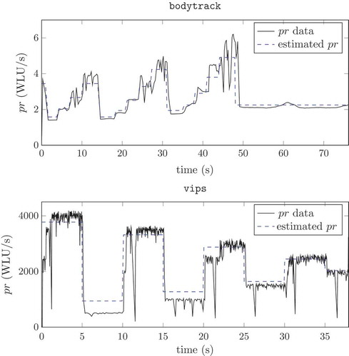
Coming to some examples referring to benchmark applications, Figure 3 shows the bodytrack and vips measured progress rate and the one estimated with the identified simulation model (5) for a particular run, where the parameters’ behaviour was obtained by means of an Extended Least Squares procedure. The used applications are bodytrack and vips, taken from the PARSEC benchmark suite. The rationale behind the suite, together with its use, is presented in [34], to which the interested reader is referred for details.

Figure 4 conversely shows the outcome of the classical black box identification process, using the ARX (AutoRegressive with eXogenous input) and the ARMAX (AutoRegressive and Moving Average with eXogenous input) model structures for a run of the vips application.

Figure 3 illustrates that Equation (5) is actually capable of replicating the data, by catching main variabilities and trends in a way suitable for control design – its sole purpose here. Figure 4 also suggests that AR(MA)X models are not keen to capture the relevant application behaviour. In fact, if one tries to identify the same data with the Matlab Identification toolbox, performing an order selection for the ARX(n_a, n_b) model, the result is that the identification procedure tries to give to the model as much higher an order as it can, indicating that the structural choice is not adequate.

For completeness, the grey box model (5) used in the presented examples, denoting with $\hat{\vartheta }$ the estimated parameter vector is parametrized for vips as

$\widehat{\vartheta }{}_{vips}=\left[\begin{array}{c}{k}_c\\ {\alpha }_c\\ o_c\end{array}\right]=\left[\begin{array}{c}258.75388\\ 1.1930687\\ 681.67218\end{array}\right],$

and for bodytrack as

${\hat{\vartheta }}_{\mathtt{b}\mathtt{o}\mathtt{d}\mathtt{y}\mathtt{t}\mathtt{r}\mathtt{a}\mathtt{c}\mathtt{k}}=\left[\begin{array}{c}{k}_c\\ {\alpha }_c\\ o_c\\ k_f\\ {\alpha }_f\\ o_f\end{array}\right]=\left[\begin{array}{c}0.1931659\\ 1.613834\\ 3.5964752\\ 2.3736936\\ 0.1609101\\ -1.9965658\end{array}\right].$

Figure 3. Collected data from the specified software application (black solid line) and simulation with the grey box identified model (blue dashed line).

In addition, by introducing a fit measure, the obtained models can be ranked. The fit measure allows to determine how close the output of the estimation is to the real process that it models. Here, the measure is set to

$\left[1-\frac{{∥Y-\hat{Y}∥}_2}{{∥Y-\bar{Y}∥}_2}\right]\cdot 100$

where $\hat{Y}$ is the output of the estimators and Y is the measure of the real data. Table 1 shows the obtained results in the vips case.

Notice that, starting from the system insight induced by the grey box model, successful adaptive control could be achieved with an ARX(1,1) structure.

Figure 4. Identification results for the vips software application with different model structures. The data used for the identification are denoted with a solid line, the simulation results of the ARMAX (10, 10, 10) with a dashed-dotted line, the ARX (30, 30) with a densely dotted line, the ARX (20, 20) with a densely dashed line, the ARX (10, 10) with a densely dotted line, and the ARX (1, 1) with a dashed line.

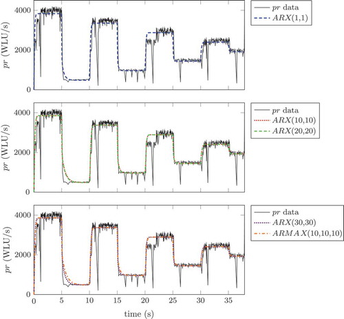
Table 1. Results obtained with the Matlab identification Toolbox for the vips application with various model structures.

Model	Delay	Best Fits
ARMAX (l0, l0, l0)	L	62.24
ARX (30, 30)	9	6l.63
ARX (20, 20)	9	6l.53
ARX (l0, l0)	9	6l.36
ARX (l, l)	L	58.98

To end this section with some control-related material, an example is presented on what can be achieved in that respect. Figure 5 shows experimental results performed on the same real applications, that is, bodytrack and vips, when their progress is regulated by an adaptive predictive controller based on model (5).

As can be seen, the required set point is well attained also in the presence of application behaviour’s variations, thus proving the effectiveness of the underlying modelling approach.

It is worth mentioning that in the resource allocation literature, using mathematical models for the allocator design is not the typical case, and heuristics or reinforcement learning – model-free – techniques are preferred [33]. This is an acceptable approach whenever the problem at hand is quite complex or difficult to manage, but if a (relatively small) effort in the modelling phase is spent, many model-based control techniques can be adopted obtaining much better results. Figure 6 shows the results that can be obtained with vips controlled with different techniques [33], that is, a heuristic one (top row), a State-Action-Reward-State-Action algorithm (second row), an adaptive control scheme (third row) and a MPC technique (bottom row). Those techniques were designed to manage both Single Resource (SR) and Multiple Resource (MR) case.

Figure 5. Experimental control results with bodytrack and vips: the application progress rate is required to attain a specified set point value.

As can be noticed, in the case of model-free techniques, the achieved performance are worse than in the case of model-based ones, evidencing that spending some effort in the modelling phase can significantly improve the control results – recall that the experiments were conducted on real applications. It is also evident that in the MPC example, the controller adapts to exploit the presence of multiple resources, and will need more time to accomplish its task. On the contrary, using a single resource (SR) greatly improve the convergence rate. However, it has to be noted that the multiple resource (SR) controllers tend to settle in states that are more power hungry than its multiple resource counterparts. However, minimizing power consumption falls outside the scope of this paper and should be investigated more.

Figure 6. Experimental results with different model-based/non-model-based techniques. Note: SARSA, State-Action-Reward-State-Action; MPC, Model Predictive Control.

6. Retrospect and future directions

We have presented different case studies on the use of discrete-time dynamic models for a control-oriented design of computing system components. It is now the time to collect and organize the so gathered experience and make some general statements.

If one approaches computing systems for modelling – and possibly control – purposes, the paradigms that naturally appear most keen to be applied are undoubtedly event-based. A vast literature is available on the use of queue networks, automata and the like [11,35,36]. In our opinion, this is less general than one may think at a first glance. There are cases – probably more than those mentioned herein – where it is more convenient to identify some phenomenon that can be described with discrete-time models, and proceed accordingly as here exemplified. Quite frequently, the involved models are simple, sometimes even linear and time invariant. Such simple models (think again to the linear case) allow for a rigorous analysis of stability, reachability, controllability and similar structural properties.

Furthermore, this simplification is also based on the idea of using discrete-time but not (necessarily) sampled-signals models. One could well say that this is a viable way of dealing with events by using a modelling paradigm with more powerful design and assessment tools.

Finally, since we aim at modelling phenomena occurring in computing systems more than components of those systems, the approach naturally leads to address both control and design problems – or more precisely, to view the matter as process/control co-design.

The considerations above allow to establish quite a deep relationship between modelling and control for computing systems, and for other application domains like industrial processes. Sticking to this example, it is well known that some phenomena and control objectives are best dealt with time-driven models, while others call for event-based ones. Correspondingly, a vast literature is available on how to structure a complete (process) control strategy comprising both time- and event-based elements, coordinated in a view to attaining the general objectives for the problem at hand. We suggest that the same approach be applied to computing systems, as attempting to stick to only one of the two mentioned paradigms quite often makes the problem hard to tackle, and often limits the achievable results.

7. Conclusions and future work

This work proposed a novel approach to the modelling of computing systems. The main idea behind this approach is to capture the relevant dynamics of computing systems with the simplest possible models, grounded on some ‘physical’ principles. The approach was shown at work with three case studies, and some general ideas were drawn from that experience.

Along this research line, future developments can be foreseen as the application of the presented ideas to other computing system problems, like, for example, bandwidth allocation. Much further work is required, but an innovative attempt was here made to circumvent one of the main obstacles for co-design success. This attempt is possibly a starting point to rethink from scratch core functionalities of computing systems with a model-based and control-theoretical attitude.

Additional information

Funding

This work was partially supported by the Swedish Research Council (VR) [grant number C0590801 (2012-5908)] for the projects ‘Cloud Control’ and ‘Power and temperature control for large-scale computing infrastructures’, and through the LCCC Linnaeus and ELLIIT Excellence Centers.

Notes

1. In the scheduler case, to stick to the example, the phenomenon is how the CPU is distributed among the running tasks. Such distribution depends on control actions, that is, on the time slice allotted to each task at each scheduler’s intervention and on exogenous disturbances, such as task blockings, resource contentions and so on.

References

- J.O. Kephart and D.M. Chess, The vision of autonomic computing, Computer 36 (1) (2003), pp. 41–50. doi:10.1109/MC.2003.1160055.
- A. Leva, M. Maggio, A.V. Papadopoulos, and F. Terraneo, Control-Based Operating System Design, IET Control Engineering Series, IET, London, June 2013. ISBN 978-1-84919-609-3.
- L. Torvalds and D. Diamond, Just for Fun: The Story of an Accidental Revolutionary, HarperBusiness, New York, 2002.
- S. Dobson, R. Sterritt, P. Nixon, and M. Hinchey, Fulfilling the vision of autonomic computing, Computer 43 (1) (2010), pp. 35–41. doi:10.1109/MC.2010.14.
- A.V. Papadopoulos, M. Maggio, and A. Leva, Control and design of computing systems: What to model and how, in Proceedings of the 7th International Conference of Mathematical Modelling, MATHMOD’12, Vol. 7, I. Troch and F. Breitenecker, eds., IFAC, Vienna, February 2012, pp. 102–107. Available at http://www.ifac-papersonline.net/Detailed/58551.html
- P. Ramadge and W. Wonham, Supervisory control of a class of discrete event processes, SIAM J. Control Optim. 25 (1) (1987), pp. 206–230. doi:10.1137/0325013.
- W. Wonham and P. Ramadge, Modular supervisory control of discrete-event systems, Math. Control Signal. 1 (1) (1988), pp. 13–30. doi:10.1007/BF02551233.
- T. Abdelzaher, J. Stankovic, C. Lu, R. Zhang, and Y. Lu, Feedback performance control in software services—Using a control-theoretic approach to achieve quality of service guarantees, IEEE Control Syst. Magazine 23 (2003), pp. 74–90. doi:10.1109/MCS.2003.1200252.
- Y. Diao, J. Hellerstein, S. Parekh, R. Griffith, G. Kaiser, and D. Phung, A control theory foundation for self-managing computing systems, IEEE J. Selected Area. Commun. 23 (12) (2005), pp. 2213–2222. doi:10.1109/JSAC.2005.857206.
- T. Patikirikorala, A. Colman, J. Han, and L. Wang, A systematic survey on the design of self-adaptive software systems using control engineering approaches, in 2012 ICSE Workshop on Software Engineering for Adaptive and Self-Managing Systems (SEAMS), IEEE, Zurich, 2012, pp. 33–42. doi:10.1109/SEAMS.2012.6224389.
- M. Shor, K. Li, J. Walpole, D. Steere, and C. Pu, Application of control theory to modeling and analysis of computer systems, Proceedings of Japan-USA-Vietnam Workshop on Research and Education in Systems, Computation and Control Engineering, HoChiMinh City, 7–9 June 2000. Available at http://archives.pdx.edu/ds/psu/10394.
- J.L. Hellerstein, Y. Diao, S. Parekh, and D.M. Tilbury, Feedback Control of Computing Systems, Wiley, New York, 2004.
- K. Lindqvist and H. Hjalmarsson, Identification for control: adaptive input design using convex optimization, Proceedings of the 40th IEEE Conference on Decision and Control, 2001, Vol. 5, 2001, pp. 4326–4331.
- M. Pinedo, Scheduling Theory, Algorithms, and Systems, 3rd ed., Springer, Berlin, 2008.
- A. Leva and M. Maggio, Feedback process scheduling with simple discrete-time control structures, IET Control Theory Appl. 4 (11) (2010), pp. 2331–2342. doi:10.1049/iet-cta.2009.0260.
- M. Maggio, A.V. Papadopoulos, and A. Leva, On the use of feedback control in the design of computing system components, Asian J. Control. 15 (1) (2013), pp. 31–40. ISSN 1934–6093. doi:10.1002/asjc.509.
- L. Abeni, L. Palopoli, G. Lipari, and J. Walpole, Analysis of a reservation-based feedback scheduler, in 23rd IEEE of Real-Time Systems Symposium, RTSS 2002, IEEE, San Juan, 2002, pp. 71–80. doi:10.1109/REAL.2002.1181563.
- B. Alam, M. Doja, and K. Biswas, Finding time quantum of round robin CPU scheduling algorithm using fuzzy logic, in International Conference on Computer and Electrical Engineering, 2008. ICCEE 2008, IEEE, Phuket, 2008, pp. 795–798. doi:10.1109/ICCEE.2008.89.
- G. Buttazzo and L. Abeni, Adaptive workload management through elastic scheduling, Real-Time Syst. 23 (2002), pp. 7–24. doi:10.1023/A:1015342318358.
- K.W. Batcher and R.A. Walker, Dynamic Round-Robin Task Scheduling to Reduce Cache Misses for Embedded Systems, in Proceedings of the Conference on Design, Automation and Test in Europe, DATE ’08, ACM, New York, 2008, pp. 260–263.
- W. Chow and W. Chiu, An analysis of swapping policies in virtual storage systems, IEEE T. Softw. Eng. 3 (2) (1977), pp. 150–156.
- R. Jones, Factors affecting the efficiency of a virtual memory, IEEE Trans. Comput. C-18 (11) (1969), pp. 1004–1008. doi:10.1109/T-C.1969.222570.
- L. Levy and P. Lipman, Virtual memory management in the VAX/VMS operating system, Computer 15 (3) (1982), pp. 35–41. doi:10.1109/MC.1982.1653971.
- H. Yun, G. Yao, R. Pellizzoni, M. Caccamo, and L. Sha, Memguard: Memory bandwidth reservation system for efficient performance isolation in multi-core platforms, in 19th IEEE Real-Time and Embedded Technology and Applications Symposium (RTAS), IEEE, Philadelphia, PA, 2013. doi:10.1109/RTAS.2013.6531079.
- E. Mumolo and G. Bernardis, A novel demand prefetching algorithm based on volterra adaptive prediction for virtual memory management systems, in Proceedings 30th Hawaii International Conference on System Sciences, Vol. 5, IEEE, Wailea, HI, 1997, pp. 160–167. doi:10.1109/HICSS.1997.663171.
- J. Corbet, 2.6 Swapping Behavior. Available at http://lwn.net/Articles/83588/ (Accessed 3 June 2014).
- F. Terraneo and A. Leva, Feedback-based memory management with active swap-in, Control Conference (ECC), 2013 European, IEEE, Zurich, July 2013, pp. 620–625. Available at http://ieeexplore.ieee.org/xpls/abs_all.jsp?arnumber=6669385&tag=1.
- IBM, An architectural blueprint for autonomic computing, Tech. Rep., IBM Corp., Hawthorne, NY, June 2005. Available at http://www-03.ibm.com/autonomic/pdfs/AC%20Blueprint%20White%20Paper%20V7.pdf (Accessed 22 July 2014).
- A.V. Papadopoulos, M. Maggio, S. Negro, and A. Leva, General control-theoretical framework for online resource allocation in computing systems, IET Control Theory Appl. 6 (11) (2012), pp. 1594–1602. ISSN 1751-8644. doi:10.1049/iet-cta.2011.0632.
- R. Kufrin, Measuring and improving application performance with PerfSuite, Linux J. 2005 (2005), pp. 4–10.
- B. Sprunt, The basics of performance-monitoring hardware, IEEE Micro. 22 (4) (2002), pp. 64–71. doi:10.1109/MM.2002.1028477.
- H. Hoffmann, J. Eastep, M.D. Santambrogio, J.E. Miller, and A. Agarwal, Application heartbeats: a generic interface for specifying program performance and goals in autonomous computing environments, Proceeding of the 7th International Conference on Autonomic Computing, ACM Press, New York, 2010, pp. 79–88.
- M. Maggio, H. Hoffmann, A.V. Papadopoulos, J. Panerati, M.D. Santambrogio, A. Agarwal, and A. Leva, Comparison of decision-making strategies for self-optimization in autonomic computing systems, ACM Trans Auton. Adap. Syst. 7 (4) (2012), pp. 1–32. ISSN 1556-4665. doi:10.1145/2382570.2382572.
- C. Bienia, S. Kumar, J.P. Singh, and K. Li, The PARSEC benchmark suite: Characterization and architectural implications, in Proceedings of the 17th International Conference on Parallel Architectures and Compilation Techniques, ACM, Toronto, October 2008. doi:10.1145/1454115.1454128.
- M.A. Kjær and A. Robertsson, Analysis of buffer delay in web-server control, American Control Conference (ACC), 2010, Baltimore, MD, June 2010, pp. 1047–1052. doi:10.1109/ACC.2010.5530756.
- A. Robertsson, B. Wittenmark, M. Kihl, and M. Andersson, Design and evaluation of load control in web server systems, in Proceedings of the 2004 American Control Conference, Vol. 3, IEEE, Boston, MA, 2004, pp. 1980–1985.