STABLE – a stability algorithm for parametric model reduction by matrix interpolation

ABSTRACT

In this article, an algorithm guaranteeing asymptotic stability for parametric model order reduction by matrix interpolation is proposed for the general class of high-dimensional linear time-invariant systems. In the first step, the system matrices of the high-dimensional parameter-dependent system are computed for a set of parameter vectors. The local high-order systems are reduced by a projection-based reduction method and stabilized, if necessary. Secondly, the low-order systems are transformed into a consistent set of generalized coordinates. Thirdly, a new procedure using semidefinite programming is applied to the low-order systems, converting them into strictly dissipative form. Finally, an asymptotically stable reduced order model can be calculated for any new parameter vector of interest by interpolating the system matrices of the local low-order models. We show that this approach works without any limiting conditions concerning the structure of the large-scale model and is suitable for real-time applications. The method is illustrated by two numerical examples.

KEYWORDS:

• Parametric model order reduction
• matrix interpolation
• stability preservation
• semidefinite programming

1. Introduction

Accurate modelling of dynamical systems can lead to large-scale systems of ordinary differential equations. If these systems are used for the purpose of optimization, simulation or control, even powerful computer systems reach their limitations, especially concerning execution time and available memory. As a remedy, methods of model order reduction (MOR) have been developed which approximate the input–output behaviour of the original system by a low-order one [1]. In addition, properties of the high-order system like stability, passivity or the Port-Hamiltonian structure should be preserved, see, e.g., [2,3]. For many engineering applications, the high-order system additionally depends on parameters, such as material parameters. For this case, methods of parametric MOR (pMOR) have been developed [4]. They construct a low-order system that approximates the large-scale one for the entire parameter domain. Hence, one can obtain a reduced system for every parameter value of the domain without the need to repeat the reduction procedure.

Besides other pMOR methods, interpolation-based methods were suggested in the literature. One approach is the interpolation of reduced system matrices [5–10], which can handle arbitrary parametric dependencies and has a low computational effort. However, it does not necessarily lead to asymptotically stable interpolated systems. Hence, some stability-preserving approaches were proposed for matrix interpolation, most of them being restricted to systems showing certain conditions concerning the structure of the large-scale model. In [5], stable interpolation on matrix manifolds is proposed for systems of ordinary differential equations in second-order form. Stability-preserving matrix interpolation for dissipative systems is suggested in [11], for Port-Hamiltonian systems in [12] and for passive systems in [13,14]. Concerning the general class of linear time-invariant (LTI) systems, a technique is suggested in [15,16] for passivity-preserving parameterized MOR which exploits the solution of high-order linear matrix inequalities (LMIs). Some stability-preserving methods are proposed in [11,17] for the general class of LTI systems. These approaches have in common that they modify one of the two reduced order bases (ROBs) of the local systems to enforce stability for the interpolated systems. The approach from [11] requires the solution of high-dimensional generalized Lyapunov equations, which is computationally very expensive. The method from [17] determines an optimal stabilizing solution with regard to a quality function that is found by solving high-order optimization problems. For reducing the computational effort, the authors also propose low-order but suboptimal optimization problems.

In the following, a procedure for stability-preserving pMOR for the general class of parameter-dependent, LTI systems is presented, where all steps of the (stability-preserving) matrix interpolation are exclusively performed in low-dimensional vectors and matrices. Preliminary studies for the proposed method were published in [18], and a detailed description can also be found in the dissertation [7]. The method starts with optimization steps similar to [17]. However, it searches for the modified ROBs in the available low-order subspaces, and hence, the optimization steps can be done very efficiently.

A short overview of MOR and pMOR by matrix interpolation is given in Section 2. The new stability-preserving method is presented in Section 3 and is compared to an existing approach in Section 4. Numerical results are presented in Section 5.

2. Preliminaries

2.1. Parameter-dependent LTI systems

In this article,¹ we consider a parameter-dependent, LTI and high-dimensional system of order n. Its representation in the time domain is

(1) $G(t,p):\{\begin{array}{ll}E(p)\dot{x}(t,p)\hfill & =A(p)x(t,p)+B(p)u(t)\hfill \\ y(t,p)\hfill & =C(p)x(t,p),\hfill \end{array}$(1)

where $\mathbf{E}(p)\in {\mathbb{R}}^{n\times n}$, $\mathbf{A}(p)\in {\mathbb{R}}^{n\times n}$, $\mathbf{B}(p)\in {\mathbb{R}}^{n\times r}$ and $\mathbf{C}(p)\in {\mathbb{R}}^{m\times n}$ are the system matrices which depend on the parameter vector $p\in \mathcal{D}$ with domain $\mathcal{D}\subseteq {\mathbb{R}}^d$. The vectors $\mathbf{u}(t)\in {\mathbb{R}}^r$, $y(t,p)\in {\mathbb{R}}^m$ and $x(t,p)\in {\mathbb{R}}^n$ denote the inputs, outputs and states of the system at time $t$, respectively. The initial value of the state vector is $x(0,p)=x_0(p)$. Performing a Laplace transformation on system (Equation (1)) and setting $x_0(p)={\mathbf{0}}_n$, we obtain the representation of the system in the frequency domain.

(2) $\mathbf{G}(s,p)=\mathbf{C}(p)[s\mathbf{E}(p)-\mathbf{A}(p){]}^{-1}\mathbf{B}(p),$(2)

where s ∈ μ is the complex frequency. When we refer to the system independent from its representation, it is denoted by G(p) in the following.

2.2. Asymptotic stability

Stability is an important property of system (Equation (1)). There exist various stability definitions [1,19,20]. In this article, the following concept of stability is examined.

Definition 2.1: The system (Equation (1)) is said to be asymptotically stable if one finds $\underset{t\to \mathrm{\infty }}{\mathrm{l}\mathrm{i}\mathrm{m}}x(t,p)={\mathbf{0}}_n$ for all initial conditions $x_0(p)$.

The following theorem gives necessary and sufficient conditions.

Theorem 2.2 ([21]): The system (Equation (1)) with non-singular $\mathbf{E}(p)$ is asymptotically stable if and only if

• S1: there exists a Lyapunov function, i.e. a function $V(x(t,p)):{\mathbb{R}}^n\to \mathbb{R}$ with $V(x(t,p))>0$ and $\dot{V}(x(t,p))<0$ for all $x(t,p)\ne {\mathbf{0}}_n$.

• S2: the eigenvalues of the pencil $(\mathbf{A}(p),\mathbf{E}(p))$ lie in the open left half of the complex plane.

A special class of systems is of particular interest in this article.

Definition 2.3 ([22]): The system (Equation (1)) is said to be strictly dissipative if it satisfies $\mathbf{E}(p)>{\mathbf{0}}_{n\times n}$ and $\mathbf{A}(p)+\mathbf{A}(p{)}^T<{\mathbf{0}}_{n\times n}$.

A strictly dissipative system possesses the Lyapunov function $V(x(t,p))=x(t,p{)}^T\mathbf{E}(p)x(t,p)$ and hence is asymptotically stable [23]. Strictly dissipative systems have the following interesting property which will be used in Section 3.3 for proposing a stability-preserving interpolation method.

Corollary 2.4 ([11,17]): Given the strictly dissipative systems $\mathbf{G}(p_1),\dots ,\mathbf{G}(p_N)$ with $\mathbf{E}(p_i)>{\mathbf{0}}_{n\times n}$ and $\mathbf{A}(p_i)+\mathbf{A}(p_i{)}^T<{\mathbf{0}}_{n\times n}$ for $i\in \{1,\dots ,N\}$, the system obtained by the superposition of the system matrices $\mathbf{A}(p)={\sum }_{i=1}^N{\omega }_i(p)\mathbf{A}(p_i)$ and $\mathbf{E}(p)={\sum }_{i=1}^N{\omega }_i(p)\mathbf{E}(p_i)$ with weighting functions ${\omega }_i:\mathcal{D}\to {\mathbb{R}}_0^{+}$ and at least one ${\omega }_i:\mathcal{D}\to {\mathbb{R}}^{+}$ possesses the Lyapunov function $V(x(t,p))=x(t,p{)}^T\mathbf{E}(p)x(t,p)$ and hence is asymptotically stable according to criterion S1 from Theorem 2.2.

2.3. Projection-based MOR

Imagine that we compute the parametric system $\mathbf{G}(p)$ for a set of grid points $p_i\in \mathcal{D}$ with $i\in \{1,\dots ,N\}$. We denote $\mathbf{E}(p_i)$ by ${\mathbf{E}}_i$ and similarly for the other matrices and the resulting non-parametric system is denoted by ${\mathbf{G}}_i:=\mathbf{G}(p_i)$ with $x_i(t):=x(t,p_i)$ and $y_i(t):=y(t,p_i)$. Then, the goal of MOR is to find a low-dimensional system ${\hat{\mathbf{G}}}_i$ of order $q\ll n$ whose output is a good approximation of the output of the original system ${\mathbf{G}}_i$, i.e., ${\hat{y}}_i(t)\approx y_i(t)$ when the same input is fed to the systems. For this, projection matrices ${\mathbf{V}}_i:=\mathbf{V}(p_i)\in {\mathbb{R}}^{n\times q}$ and ${\mathbf{W}}_i:=\mathbf{W}(p_i)\in {\mathbb{R}}^{n\times q}$, which are referred to as ROBs, are calculated. The case ${\mathbf{W}}_i={\mathbf{V}}_i$ is called one-sided reduction and the case ${\mathbf{W}}_i\ne {\mathbf{V}}_i$ is referred to as two-sided reduction. The ROBs span the right ${\mathcal{V}}_i=\mathrm{s}\mathrm{p}\mathrm{a}\mathrm{n}({\mathbf{V}}_i)$ and left subspace ${\mathcal{W}}_i=\mathrm{s}\mathrm{p}\mathrm{a}\mathrm{n}({\mathbf{W}}_i)$, respectively. For the calculation of the ROBs, we can apply projection-based reduction methods such as Krylov subspace methods, truncated balanced realization (TBR) or proper orthogonal decomposition, see, e.g., [1] and references therein. Using the approximation $x_i(t)\approx {\mathbf{V}}_i{\hat{x}}_i(t)$ with the reduced state vector ${\hat{x}}_i(t)\in {\mathbb{R}}^q$ and enforcing the Petrov–Galerkin condition

(3) $W_i^T(E_i{V}_i{\dot{\widehat{x}}}_i(t)-A_i{V}_i{\widehat{x}}_i(t)-B_{i}u(t))=0,$(3)

leads to the reduced order model

(4) ${\widehat{G}}_i:\{\begin{array}{ll}{\widehat{E}}_i{\dot{\widehat{x}}}_i(t)\hfill & ={\widehat{A}}_i{\widehat{x}}_i(t)+{\widehat{B}}_{i}u(t)\hfill \\ {\widehat{y}}_i(t)\hfill & ={\widehat{C}}_i{\widehat{x}}_i(t),\hfill \end{array}$(4)

where the reduced system matrices are given by

(5) ${\hat{\mathbf{E}}}_i={\mathbf{W}}_i^T{\mathbf{E}}_i{\mathbf{V}}_i,{\hat{\mathbf{A}}}_i={\mathbf{W}}_i^T{\mathbf{A}}_i{\mathbf{V}}_i,{\hat{\mathbf{B}}}_i={\mathbf{W}}_i^T{\mathbf{B}}_i,{\hat{\mathbf{C}}}_i={\mathbf{C}}_i{\mathbf{V}}_i.$(5)

2.4. Parametric MOR by matrix interpolation

Methods of pMOR have been developed to approximate the parameter-dependent, high-order system $\mathbf{G}(p)$ while preserving the parameter-dependency in the reduced-order model. The method of interest in this article interpolates precomputed reduced system matrices. It was proposed in [5,6,9,10] and a unifying framework was suggested in [7,8]. We sum up four preprocessing steps (offline phase) and the interpolation step (online phase).

1. The domain μ is sampled for a set of vectors $\mathcal{P}=\{p_1,\dots ,p_N\}\subset \mathcal{D}$ with $N=|\mathcal{P}|$. Then, the system $\mathbf{G}(p)$ is computed for the vectors in the set $\mathcal{P}$ which results in a set of high-order systems $\mathcal{G}=\{\mathbf{G}(p_1),\dots ,\mathbf{G}(p_N)\}$.

2. Each system in the set μ is reduced individually to order $q\ll n$, where any projection-based reduction method can be applied according to Section 2.3 resulting in a set of low-order systems $\hat{\mathcal{G}}=\{\hat{\mathbf{G}}(p_1),\dots ,\hat{\mathbf{G}}(p_N)\}$.

3. The reduced systems of the set $\hat{\mathcal{G}}$ have different bases ${\mathbf{V}}_1,\dots ,{\mathbf{V}}_N$. These right ROBs need to be adjusted to the basis of the reference subspace ${\mathbf{V}}_0$. An approach that captures the most important directions of all subspaces and has a low computational effort uses the economy version of the SVD

   (6) $\begin{array}{l}{U}_V{\text{S}}_V{Z}_V^T=\text{svd}([V_1,\dots ,V_N],\text{'}\text{econ}\text{'})\Rightarrow V_0=U_V(:,1:q).\hfill \end{array}$(6)

   The right ROBs are transformed for $i\in \{1,\dots ,N\}$ with matrices ${\mathbf{T}}_i\in {\mathbb{R}}^{q\times q}$ to ${\tilde{\mathbf{V}}}_i={\mathbf{V}}_i{\mathbf{T}}_i$ so that a quality function is minimized. A possible quality function is the modal assurance criterion (MAC) between the local basis ${\tilde{\mathbf{V}}}_i$ and the reference basis ${\mathbf{V}}_0$ which can be written according to [7,24]

   (7) $J_{\mathrm{M}\mathrm{A}\mathrm{C},\mathbf{V},i}({\mathbf{T}}_i)=\parallel {\mathbf{V}}_0^T{\tilde{\mathbf{V}}}_i-{\mathbf{I}}_q{\parallel }_F=\parallel {\mathbf{V}}_0^T{\mathbf{V}}_i{\mathbf{T}}_i-{\mathbf{I}}_q{\parallel }_F.$(7)

   The solution with the minimum norm value, $J_{\mathrm{M}\mathrm{A}\mathrm{C},\mathbf{V},i}=0$, is ${\mathbf{T}}_i=({\mathbf{V}}_0^T{\mathbf{V}}_i{)}^{-1}$. A second possible quality function is the distance (DS) between the local basis ${\tilde{\mathbf{V}}}_i$ and the reference basis ${\mathbf{V}}_0$ measured in the Frobenius norm [5,7,24]

   (8) $J_{\mathrm{D}\mathrm{S},\mathbf{V},i}({\mathbf{T}}_i)=\parallel {\tilde{\mathbf{V}}}_i-{\mathbf{V}}_0{\parallel }_F=\parallel {\mathbf{V}}_i{\mathbf{T}}_i-{\mathbf{V}}_0{\parallel }_F.$(8)

   The solution with the minimum value of the cost function is ${\mathbf{T}}_i={\mathbf{V}}_i^{+}{\mathbf{V}}_0$ using the pseudoinverse ${\mathbf{V}}_i^{+}=({\mathbf{V}}_i^T{\mathbf{V}}_i{)}^{-1}{\mathbf{V}}_i^T$.

4. In analogy, the bases ${\mathbf{W}}_1,\dots ,{\mathbf{W}}_N$ need to be adjusted to the basis of the reference subspace ${\mathbf{W}}_0$, which can, e.g., be calculated according to Equation (6) by replacing the respective values. The left ROBs are transformed for $i\in \{1,\dots ,N\}$ with matrices ${\mathbf{M}}_i\in {\mathbb{R}}^{q\times q}$ to ${\tilde{\mathbf{W}}}_i={\mathbf{W}}_i{\mathbf{M}}_i$ so that a quality function is minimized. For the MAC approach, we obtain the quality function

   (9) $J_{\mathrm{M}\mathrm{A}\mathrm{C},\mathbf{W},i}({\mathbf{M}}_i)=\parallel {\mathbf{W}}_0^T{\tilde{\mathbf{W}}}_i-{\mathbf{I}}_q{\parallel }_F=\parallel {\mathbf{W}}_0^T{\mathbf{W}}_i{\mathbf{M}}_i-{\mathbf{I}}_q{\parallel }_F$(9)

with the optimal solution ${\mathbf{M}}_i=({\mathbf{W}}_0^T{\mathbf{W}}_i{)}^{-1}$. For the DS approach, we obtain

(10) $J_{\mathrm{D}\mathrm{S},\mathbf{W},i}({\mathbf{M}}_i)=\parallel {\tilde{\mathbf{W}}}_i-{\mathbf{W}}_0{\parallel }_F=\parallel {\mathbf{W}}_i{\mathbf{M}}_i-{\mathbf{W}}_0{\parallel }_F$(10)

with the optimal solution ${\mathbf{M}}_i={\mathbf{W}}_i^{+}{\mathbf{W}}_0$.

The steps discussed so far are performed in the offline phase and have to be done only once. They result in a set of reduced-order systems $\tilde{\mathcal{G}}=\{{\tilde{\mathbf{G}}}_1,\dots ,{\tilde{\mathbf{G}}}_N\}$ with

(11) ${\tilde{G}}_i:\{\begin{array}{ll}\stackrel{{\tilde{E}}_i}{\overbrace{M_i^T{\widehat{E}}_i{T}_i}}{\dot{\tilde{x}}}_i(t)\hfill & =\stackrel{{\tilde{A}}_i}{\overbrace{M_i^T{\widehat{A}}_i{T}_i}}{\dot{\tilde{x}}}_i(t)+\stackrel{{\tilde{B}}_i}{\overbrace{M_i^T{\widehat{B}}_i}}u(t)\hfill \\ {\tilde{y}}_i(t)\hfill & =\underset{C_i}{\underbrace{{\widehat{C}}_i{T}_i}}{\tilde{x}}_i(t).\hfill \end{array}$(11)

Note that these systems differ from systems (Equation (4)) only in their state-space representation, but not in their eigenvalues or input–output behaviour.

In the online phase, i.e. when a reduced order model for the new parameter vector $p\in \mathcal{D}$ is supposed to be calculated, this is simply done by the interpolation of the precomputed matrices with weighting functions ${\omega }_1,\dots ,{\omega }_N:\mathcal{D}\to \mathbb{R}$. Then, the new reduced system for the parameter vector $p$ is obtained by

(12) $\tilde{G}(p):\{\begin{array}{ll}\tilde{E}(p)\dot{\tilde{x}}(t,p)\hfill & =\tilde{A}(p)\tilde{x}(t,p)+\tilde{B}(p)u(t)\hfill \\ \tilde{y}(t,p)\hfill & =\tilde{C}(p)\tilde{x}(t,p)\hfill \end{array}$(12)

with

(13) $\begin{array}{cc}\tilde{\mathbf{E}}(p)& ={\sum }_{i=1}^N{\omega }_i(p){\tilde{\mathbf{E}}}_i,\tilde{\mathbf{A}}(p)={\sum }_{i=1}^N{\omega }_i(p){\tilde{\mathbf{A}}}_i,\\ \tilde{\mathbf{B}}(p)& ={\sum }_{i=1}^N{\omega }_i(p){\tilde{\mathbf{B}}}_i,\tilde{\mathbf{C}}(p)={\sum }_{i=1}^N{\omega }_i(p){\tilde{\mathbf{C}}}_i.\end{array}$(13)

The system matrices can also be interpolated element-wise and on matrix manifolds.

2.5. Problem formulation

The matrix interpolation (Equation (13)) does not always lead to an asymptotically stable system (Equation (12)), even if all reduced systems in the set $\tilde{\mathcal{G}}$ are asymptotically stable. In other words, the reduction (Equations (12) and (13)) does not guarantee asymptotic stability of the reduced model.

Example: Consider the two asymptotically stable systems ${\dot{\widehat{x}}}_1(t)={\widehat{A}}_1{\widehat{x}}_1(t)$ and ${\dot{\widehat{x}}}_2(t)={\widehat{A}}_2{\widehat{x}}_2(t)$ with matrices

(14) ${\hat{\mathbf{A}}}_1=\left[\begin{array}{cc}-2& 5\\ 0& -2\end{array}\right],{\hat{\mathbf{A}}}_2=\left[\begin{array}{cc}-2& 0\\ 5& -2\end{array}\right].$(14)

For example, the interpolated matrix

(15) ${\hat{\mathbf{A}}}_{\mathrm{i}\mathrm{n}\mathrm{t}}=0.5{\hat{\mathbf{A}}}_1+0.5{\hat{\mathbf{A}}}_2=\left[\begin{array}{cc}-2& 2.5\\ 2.5& -2\end{array}\right]$(15)

has the spectrum {–4.5, 0.5} and the resulting system $\dot{\widehat{x}}(t)={\widehat{A}}_{\text{int}}\widehat{x}(t)$ is therefore unstable according to criterion S2 of Theorem 2.2.

An idea to solve this problem is to minimally change the left ROBs ${\tilde{\mathbf{W}}}_1,\dots ,{\tilde{\mathbf{W}}}_N$ such that the interpolated reduced system is guaranteed to be asymptotically stable.

3. Stability-preserving interpolation of reduced system matrices

3.1. Calculation of a set of asymptotically stable, reduced systems

The proposed method starts with a set of high-order systems $\mathcal{G}=\{{\mathbf{G}}_1,\dots ,{\mathbf{G}}_N\}$. These systems are reduced individually to the order $q\ll n$ according to Equation (4), and we assume that the reduced systems $\hat{\mathcal{G}}=\{{\hat{\mathbf{G}}}_1,\dots ,{\hat{\mathbf{G}}}_N\}$ are asymptotically stable. In order to ensure this stability, two general approaches are possible: (i) We can use stability-preserving reduction methods such as TBR or extended versions of Krylov subspace methods. (For the latter, the stability-preserving, adaptive rational Krylov (SPARK) from [25] guarantees stability and the iterative rational Krylov algorithm (IRKA) from [26] delivers asymptotically stable systems as long as it converges.) (ii) For MOR methods that do not implicitly guarantee stability, one can easily check if the reduced systems are asymptotically stable by examining their eigenvalues according to criterion S2 from Theorem 2.2; if a system is then found to be unstable, it can be stabilized via post-processing, e.g. by modifying the left or right ROBs [27,28].

3.2. Adjustment of the right ROBs

The reduced systems of the set $\hat{\mathcal{G}}$ have different bases ${\mathbf{V}}_1,\dots ,{\mathbf{V}}_N$ and it was shown in Section 2.4 that they need to be adjusted to the basis of the reference subspace for accuracy reasons. For this, the right ROBs are transformed for $i\in \{1,\dots ,N\}$ to ${\tilde{\mathbf{V}}}_i={\mathbf{V}}_i{\mathbf{T}}_i$ with ${\mathbf{T}}_i=({\mathbf{V}}_0^T{\mathbf{V}}_i{)}^{-1}$ using the MAC approach or with ${\mathbf{T}}_i={\mathbf{V}}_i^{+}{\mathbf{V}}_0$ using the DS approach as described in Section 2.4.

3.3. Stabilizing procedure using semidefinite programming

In this section, a stabilization method is described for the interpolation of reduced matrices. The demands that we impose on the method are – besides stability preservation – accuracy and the operation on low-order systems. The main idea is the following: starting from the transformed bases ${\tilde{\mathbf{W}}}_i={\mathbf{W}}_i{\mathbf{M}}_i$ for $i\in \{1,\dots ,N\}$ with ${\mathbf{M}}_i=({\mathbf{W}}_0^T{\mathbf{W}}_i{)}^{-1}$ using the MAC approach or with ${\mathbf{M}}_i={\mathbf{W}}_i^{+}{\mathbf{W}}_0$ using the DS approach (cf. Section 2.4), we minimally modify the new left ROBs ${\tilde{\mathbf{W}}}_i$ until stability is guaranteed (again note that the eigenvalues and the input–output behaviour of the local models remain unchanged).

3.3.1. Feasibility problem

To begin with, an abstract optimization problem is formulated in which a convex objective function $J_{\mathbf{W}}$ is minimized subject to the constraint that the interpolated system $\tilde{\mathbf{G}}(p)$ is asymptotically stable for the domain $\mathcal{D}$. According to criterion S1 from Theorem 2.2, this constraint is equivalent to the existence of a Lyapunov function $V(\tilde{x}(t,p))$. Hence, we obtain the optimization problem

(16) $\mathrm{m}\mathrm{i}\mathrm{n}{J}_{\mathbf{W}}\mathrm{s}.\mathrm{t}.\mathrm{\exists }\mathrm{L}\mathrm{y}\mathrm{a}\mathrm{p}\mathrm{u}\mathrm{n}\mathrm{o}\mathrm{v}\mathrm{f}\mathrm{u}\mathrm{n}\mathrm{c}\mathrm{t}\mathrm{i}\mathrm{o}\mathrm{n}V(\tilde{x}(t,p))\mathrm{\forall }p\in \mathcal{D}.$(16)

According to Corollary 2.4, the existence of a Lyapunov function is guaranteed for the superposition of strictly dissipative systems when non-negative weighting functions are applied. Hence, the optimization problem (Equation (16)) is rewritten as $N$ problems, one for each grid point [17]. We introduce for each $i\in \{1,\dots ,N\}$ the basis ${\tilde{\mathbf{W}}}_i$ as optimization variable and we aim to calculate this variable so that the system ${\tilde{\mathbf{G}}}_i$ is strictly dissipative and the objective function $J_{\mathbf{W},i}$ reaches its minimum value:

(17) $\begin{array}{rl}& \underset{{\tilde{\mathbf{W}}}_i\in {\mathbb{R}}^{n\times q}}{min}{J}_{\mathbf{W},i}\left({\tilde{\mathbf{W}}}_i\right)\\ & \mathrm{s}.\mathrm{t}.{\tilde{\mathbf{W}}}_i^T{\mathbf{A}}_i{\tilde{\mathbf{V}}}_i+{\left({\tilde{\mathbf{W}}}_i^T{\mathbf{A}}_i{\tilde{\mathbf{V}}}_i\right)}^T<{\mathbf{0}}_{q\times q}\\ & {\tilde{\mathbf{W}}}_i^T{\mathbf{E}}_i{\tilde{\mathbf{V}}}_i>{\mathbf{0}}_{q\times q}\end{array}$(17)

Unfortunately, the matrices ${\tilde{\mathbf{W}}}_i$ are of high-order, and hence, the optimization problems are intractable. As a remedy, the new bases ${\tilde{\mathbf{W}}}_i$ are searched in the available subspaces ${\mathcal{W}}_i=\mathrm{s}\mathrm{p}\mathrm{a}\mathrm{n}\{{\mathbf{W}}_i\}$. For this, the matrices ${\mathbf{M}}_i\in {\mathbb{R}}^{q\times q}$ are introduced as new variables, which provide the new bases ${\tilde{\mathbf{W}}}_i={\mathbf{W}}_i{\mathbf{M}}_i$ and the optimization problems

(18) $\underset{{\mathbf{M}}_i\in {\mathbb{R}}^{q\times q}}{\mathrm{m}\mathrm{i}\mathrm{n}}{J}_{\mathbf{W},i}({\mathbf{M}}_i)$(18)

(19) $\mathrm{s}.\mathrm{t}.{\mathbf{M}}_i^T{\hat{\mathbf{A}}}_i{\mathbf{T}}_i+({\mathbf{M}}_i^T{\hat{\mathbf{A}}}_i{\mathbf{T}}_i{)}^T<{\mathbf{0}}_{q\times q}$(19)

(20) ${\mathbf{M}}_i^T{\hat{\mathbf{E}}}_i{\mathbf{T}}_i>{\mathbf{0}}_{q\times q}$(20)

which only contain low-order matrices. For solving these problems efficiently using interior point methods such as described, e.g., in [29], they are transformed into semidefinite programs. These kinds of optimization problems deal with symmetric positive or negative (semi)definite matrices as variables. To get to this form, the change of variables

(21) ${\mathbf{M}}_i={\mathbf{P}}_i{\hat{\mathbf{E}}}_i{\mathbf{T}}_i$(21)

is introduced, where the new variables ${\mathbf{P}}_i\in {\mathbb{S}}_q$ are symmetric matrices [21]. Then, Equation (21) is inserted into inequality (Equation (20)), which gives the necessary constraint on the definiteness of the optimization variables

(22) $\begin{array}{cc}{\mathbf{M}}_i^T{\hat{\mathbf{E}}}_i{\mathbf{T}}_i& ={\mathbf{T}}_i^T{\hat{\mathbf{E}}}_i^T{\mathbf{P}}_i{\hat{\mathbf{E}}}_i{\mathbf{T}}_i=({\hat{\mathbf{E}}}_i{\mathbf{T}}_i{)}^T{\mathbf{P}}_i({\hat{\mathbf{E}}}_i{\mathbf{T}}_i)>{\mathbf{0}}_{q\times q}\\ \hspace{0.17em}& \Rightarrow {\mathbf{P}}_i>{\mathbf{0}}_{q\times q}.\end{array}$(22)

For Equation (19) it follows

(23) $\begin{array}{cc}{\mathbf{M}}_i^T{\hat{\mathbf{A}}}_i{\mathbf{T}}_i+{({\mathbf{M}}_i^T{\hat{\mathbf{A}}}_i{\mathbf{T}}_i)}^T& ={\mathbf{T}}_i^T{\hat{\mathbf{E}}}_i^T{\mathbf{P}}_i{\hat{\mathbf{A}}}_i{\mathbf{T}}_i+{\mathbf{T}}_i^T{\hat{\mathbf{A}}}_i^T{\mathbf{P}}_i{\hat{\mathbf{E}}}_i{\mathbf{T}}_i\\ \hspace{0.17em}& ={\mathbf{T}}_i^T({\hat{\mathbf{E}}}_i^T{\mathbf{P}}_i{\hat{\mathbf{A}}}_i+{\hat{\mathbf{A}}}_i^T{\mathbf{P}}_i{\hat{\mathbf{E}}}_i){\mathbf{T}}_i<{\mathbf{0}}_{q\times q}\\ \hspace{0.17em}& \Rightarrow {\hat{\mathbf{E}}}_i^T{\mathbf{P}}_i{\hat{\mathbf{A}}}_i+{\hat{\mathbf{A}}}_i^T{\mathbf{P}}_i{\hat{\mathbf{E}}}_i<{\mathbf{0}}_{q\times q}.\end{array}$(23)

Finally, the new optimization problems are

(24) $\begin{array}{cc}\underset{{\mathbf{P}}_i\in {\mathbb{R}}_q}{min}{J}_{\mathbf{W},i}\left({\mathbf{P}}_i\right)& \hspace{0.17em}\\ \mathrm{s}.\mathrm{t}.{\hat{\mathbf{E}}}_i^T{\mathbf{P}}_i{\hat{\mathbf{A}}}_i+{\hat{\mathbf{A}}}_i^T{\mathbf{P}}_i{\hat{\mathbf{E}}}_i& <{\mathbf{0}}_{q\times q}\\ {\mathbf{P}}_i& >{\mathbf{0}}_{q\times q\cdot }\end{array}$(24)

For assessing the solvability of problems (Equation (24)), the theory of convex optimization tells us that only the constraints have to be examined and the quality function can be set to 0 which is referred to as feasibility problem [30]. In this case, the constraints are LMIs which are equivalent to the generalized Lyapunov inequality [31]. This inequality and accordingly the optimization problem (Equation (24)) admit a solution because the eigenvalues of the pencil $({\hat{\mathbf{A}}}_i,{\hat{\mathbf{E}}}_i)$ lie in the open left half of the complex plane as a result of Section 3.1.

3.3.2. Objective functions

In Section 3.3.1, the feasibility problem was introduced which guarantees stable matrix interpolation for all solutions satisfying the constraints. In this section, amongst these solutions, the optimal stabilizing one is determined with regard to an objective function. The objective function, which needs to be minimized, is chosen in such a way that we obtain an accurate matrix interpolation. For this, we can use the objective functions described in Equation (4) which adjust (for each $i\in \{1,\dots ,N\}$) the basis ${\mathbf{W}}_i$ to the basis of the reference subspace ${\mathbf{W}}_0$ by transforming it to ${\tilde{\mathbf{W}}}_i={\mathbf{W}}_i{\mathbf{M}}_i$ with ${\mathbf{M}}_i\in {\mathbb{R}}^{q\times q}$. For the MAC approach, we insert the new choice for ${\mathbf{M}}_i$ from Equation (21) into the objective function (Equation (9)) and we obtain

(25) $J_{\mathrm{M}\mathrm{A}\mathrm{C},\mathbf{W},i}({\mathbf{P}}_i)=\parallel {\mathbf{W}}_0^T{\mathbf{W}}_i{\mathbf{P}}_i{\hat{\mathbf{E}}}_i{\mathbf{T}}_i-{\mathbf{I}}_q{\parallel }_F.$(25)

The matrices ${\mathbf{X}}_i={\mathbf{W}}_0^T{\mathbf{W}}_i\in {\mathbb{R}}^{q\times q}$ and ${\mathbf{Y}}_i={\hat{\mathbf{E}}}_i{\mathbf{T}}_i\in {\mathbb{R}}^{q\times q}$ can be precomputed, and hence, the objective function that only comprises low-order matrices is obtained:

(26) $J_{\mathrm{M}\mathrm{A}\mathrm{C},\mathbf{W},i}({\mathbf{P}}_i)=\parallel {\mathbf{X}}_i{\mathbf{P}}_i{\mathbf{Y}}_i-{\mathbf{I}}_q{\parallel }_F.$(26)

This objective function is convex as the composition of the Frobenius norm, which is a convex function, with the affine map ${\mathbf{P}}_i\mapsto {\mathbf{X}}_i{\mathbf{P}}_i{\mathbf{Y}}_i-{\mathbf{I}}_q$ convex [30]. For the DS approach, we insert the new choice for ${\mathbf{M}}_i$ from Equation (21) into the objective function (Equation (10)):

(27) $J_{\mathrm{D}\mathrm{S},\mathbf{W},i}({\mathbf{P}}_i)=\parallel {\mathbf{W}}_i{\mathbf{P}}_i{\hat{\mathbf{E}}}_i{\mathbf{T}}_i-{\mathbf{W}}_0{\parallel }_F.$(27)

Unfortunately, this objective function is of large order since the matrices ${\mathbf{W}}_i,{\mathbf{W}}_0$ have the size $n\times q$. As a remedy, we take the square of the Frobenius norm, rewrite it using the trace and obtain

(28) $\begin{array}{rl}{J}_{\mathrm{D}\mathrm{S},\mathbf{W},i}({\mathbf{P}}_i{)}^2=& \parallel {\mathbf{W}}_i{\mathbf{P}}_i{\hat{\mathbf{E}}}_i{\mathbf{T}}_i-{\mathbf{W}}_0{\parallel }_F^2\\ =& \mathrm{t}\mathrm{r}({\mathbf{T}}_i^T{\hat{\mathbf{E}}}_i^T{\mathbf{P}}_i{\mathbf{W}}_i^T{\mathbf{W}}_i{\mathbf{P}}_i{\hat{\mathbf{E}}}_i{\mathbf{T}}_i)-2\mathrm{t}\mathrm{r}({\mathbf{W}}_0^T{\mathbf{W}}_i{\mathbf{P}}_i{\hat{\mathbf{E}}}_i{\mathbf{T}}_i)+\mathrm{t}\mathrm{r}({\mathbf{W}}_0^T{\mathbf{W}}_0)\\ =& \parallel ({\mathbf{W}}_i^T{\mathbf{W}}_i{)}^{1/2}{\mathbf{P}}_i{\hat{\mathbf{E}}}_i{\mathbf{T}}_i{\parallel }_F^2-2\mathrm{t}\mathrm{r}({\mathbf{W}}_0^T{\mathbf{W}}_i{\mathbf{P}}_i{\hat{\mathbf{E}}}_i{\mathbf{T}}_i)+\mathrm{t}\mathrm{r}({\mathbf{W}}_0^T{\mathbf{W}}_0).\end{array}$(28)

The low-order matrices ${\mathbf{X}}_i$, ${\mathbf{Y}}_i$ and ${\mathbf{Z}}_i=({\mathbf{W}}_i^T{\mathbf{W}}_i{)}^{1/2}\in {\mathbb{R}}^{q\times q}$ can again be precomputed. When the third, constant term is left out, the final low-order objective function is obtained:

(29) $J_{\mathrm{D}\mathrm{S},\mathbf{W},i}({\mathbf{P}}_i)=\parallel {\mathbf{Z}}_i{\mathbf{P}}_i{\mathbf{Y}}_i{\parallel }_F^2-2\mathrm{t}\mathrm{r}({\mathbf{X}}_i{\mathbf{P}}_i{\mathbf{Y}}_i).$(29)

The first term is convex because the composition of the square which is a convex, non-decreasing function for non-negative arguments and the convex Frobenius norm is convex. The entire quality function is convex as the sum of the first convex function and the trace, which is a linear function, is also convex [30].

3.3.3. Algorithm

The proposed method modifies the left ROBs for an accurate interpolation while making the local reduced models’ representations strictly dissipative and thereby guaranteeing stability of any interpolated reduced model. For this, the objective function (Equation (26) or (29)) is minimized for every grid point subject to the constraint (Equations (22) and (23)). As the objective functions are convex and the constraints are linear, a convex optimization problem is obtained which is referred to as Stability Algorithm Based on Linear Matrix Inequalities (STABLE) and which is given in Algorithm 1.

Algorithm 1 STABLE

input: Matrices ${\hat{\mathbf{E}}}_i,{\hat{\mathbf{A}}}_i,{\mathbf{T}}_i$, ${\mathbf{W}}_i$ for $i\in \{1,\dots ,N\}$, reference basis ${\mathbf{W}}_0$

output: Matrices ${\mathbf{M}}_i$ for $i\in \{1,\dots ,N\}$

1: for $i=1$ to $N$ do

2: Compute ${\mathbf{X}}_i={\mathbf{W}}_0^T{\mathbf{W}}_i$, ${\mathbf{Y}}_i={\hat{\mathbf{E}}}_i{\mathbf{T}}_i$, ${\mathbf{Z}}_i=({\mathbf{W}}_i^T{\mathbf{W}}_i{)}^{1/2}$

3: Solve the convex optimization problem (MAC or DS approach):

$\underset{{\mathbf{P}}_i\in {\mathbb{S}}_q}{\mathrm{m}\mathrm{i}\mathrm{n}}\parallel {\mathbf{X}}_i{\mathbf{P}}_i{\mathbf{Y}}_i-{\mathbf{I}}_q{\parallel }_F\mathrm{o}\mathrm{r}\underset{{\mathbf{P}}_i\in {\mathbb{S}}_q}{\mathrm{m}\mathrm{i}\mathrm{n}}(\parallel {\mathbf{Z}}_i{\mathbf{P}}_i{\mathbf{Y}}_i{\parallel }_F^2-2\mathrm{t}\mathrm{r}({\mathbf{X}}_i{\mathbf{P}}_i{\mathbf{Y}}_i))$

$\begin{array}{cc}\mathrm{s}.\mathrm{t}.{\hat{\mathbf{E}}}_i^T{\mathbf{P}}_i{\hat{\mathbf{A}}}_i+{\hat{\mathbf{A}}}_i^T{\mathbf{P}}_i{\hat{\mathbf{E}}}_i& <{\mathbf{0}}_{q\times q}\\ {\mathbf{P}}_i& >{\mathbf{0}}_{q\times q}\end{array}$

4: Compute ${\mathbf{M}}_i={\mathbf{P}}_i{\hat{\mathbf{E}}}_i{\mathbf{T}}_i$

5: end for

As STABLE is a low-order optimization problem, it can easily be implemented and solved, e.g. in MATLAB, using convex optimization solver packages that rely on semidefinite programming such as CVX [32,33]. These packages are based on algorithms which solve an optimization problem iteratively. According to, e.g., [29,31,34–36], the complexity is at most $\mathcal{O}(q^6)$ per iteration and in practice the solvers perform much better. The required number of iterations can be considered in practice almost independent of the problem size, ranging between 5 and 50, as long as the numerics is kept well-conditioned. Hence, the solution of the semidefinite programs is currently restricted to sizes for the reduced order $q$ up to some hundreds.

Then, STABLE delivers for each $i\in \{1,\dots ,N\}$ the transformation matrix ${\mathbf{M}}_i$ which results in the strictly dissipative reduced system ${\tilde{\mathbf{G}}}_i$ with ${\tilde{\mathbf{E}}}_i>{\mathbf{0}}_{q\times q}$ and ${\tilde{\mathbf{A}}}_i+{\tilde{\mathbf{A}}}_i^T<{\mathbf{0}}_{q\times q}$. This ensures asymptotic stability of any interpolated reduced model, according to Corollary 2.4. The price paid is a slight increase of the minimum value of the objective function since the left ROBs are distorted as little as possible compared to the method from Section 2.4. For the case that the feasibility problem (Equation (24)) only allows a very limited solution set, one might obtain a more distinct distortion of the left ROBs, which can lead to noticeable interpolation errors.

Remark 3.1 In a dual way, we could adjust the left ROBs for accuracy reasons such as described in Section 2.4 and solve an optimization problem in order to modify the right ROBs for an accurate interpolation while preserving the stability, see dissertation [7] for detailed information.

3.4. Online interpolation process

In the online phase, the reduced order model $\tilde{\mathbf{G}}(p)$ for a new parameter $p\in \mathcal{D}$ is computed by interpolation of the precomputed matrices as in Equation (13). Following Corollary 2.4, the interpolation process needs to take place with non-negative weighting functions ${\omega }_1,\dots ,{\omega }_N:\mathcal{D}\to {\mathbb{R}}_0^{+}$ and a positive weighting function ${\omega }_i:\mathcal{D}\to {\mathbb{R}}^{+}$ for at least one $i\in \{1,\dots ,N\}$. One example for such weighting functions are linear basis functions. Then, the interpolated system $\tilde{\mathbf{G}}(p)$ possesses the Lyapunov function $V(\tilde{x}(t,p))=\tilde{x}(t,p{)}^T({\sum }_{i=1}^N{\omega }_i(p){\tilde{\mathbf{E}}}_i)\tilde{x}(t,p)$ and hence is asymptotically stable for the entire domain $\mathcal{D}$.

4. Comparison to an approach in the literature

A method is proposed in [11] which guarantees stable interpolation of reduced system matrices for the special case of strictly dissipative high-order systems. It applies for each $i\in \{1,\dots ,N\}$ the one-sided reduction ${\mathbf{W}}_i={\mathbf{V}}_i$, adjusts the right ROB with ${\mathbf{T}}_i=({\mathbf{V}}_0^T{\mathbf{V}}_i{)}^{-1}$ and chooses for the left ROB the matrices ${\mathbf{M}}_i={\mathbf{T}}_i$.

Proposition 4.1: STABLE comprises the method from [11] as a special case for strictly dissipative systems and extends it to the general class of LTI systems.

Proof. For high-order system, ${\mathbf{G}}_i$ with ${\mathbf{E}}_i>{\mathbf{0}}_{n\times n}$ and ${\mathbf{A}}_i+{\mathbf{A}}_i^T<{\mathbf{0}}_{n\times n}$ perform a one-sided reduction method with ${\mathbf{W}}_i={\mathbf{V}}_i$, which leads to a reduced system fulfilling ${\hat{\mathbf{E}}}_i>{\mathbf{0}}_{q\times q}$ and ${\hat{\mathbf{A}}}_i+{\hat{\mathbf{A}}}_i^T<{\mathbf{0}}_{q\times q}$ [23]. For the adjustment of the right ROBs, just like in [11], take the matrix ${\mathbf{T}}_i=({\mathbf{V}}_0^T{\mathbf{V}}_i{)}^{-1}$ which corresponds to the MAC approach (Equation (27)). For adjusting the left ROBs, we consider the objective function (Equation (25))

$\begin{array}{c}{J}_{\mathrm{M}\mathrm{A}\mathrm{C},\mathbf{W},i}({\mathbf{P}}_i)=\parallel {\mathbf{V}}_0^T{\mathbf{V}}_i{\mathbf{P}}_i{\hat{\mathbf{E}}}_i{\mathbf{T}}_i-{\mathbf{I}}_q{\parallel }_F=\parallel {\mathbf{T}}_i^{-1}{\mathbf{P}}_i{\hat{\mathbf{E}}}_i{\mathbf{T}}_i-{\mathbf{I}}_q{\parallel }_F\end{array}$

which reaches its minimum value, $J_{\mathrm{M}\mathrm{A}\mathrm{C},\mathbf{W},i}=0$, for ${\mathbf{P}}_i={\hat{\mathbf{E}}}^{-1}$. The same holds true for the objective function of the DS approach (Equation (27)). The optimal solution belongs to the feasible set because it fulfils the first constraint (Equation (22)) owing to

${\mathbf{P}}_i={\hat{\mathbf{E}}}_i^{-1}>{\mathbf{0}}_{q\times q}$

and the second constraint (Equation (23)) because of

$\begin{array}{c}{\hat{\mathbf{E}}}_i^T{\mathbf{P}}_i{\hat{\mathbf{A}}}_i+{\hat{\mathbf{A}}}_i^T{\mathbf{P}}_i{\hat{\mathbf{E}}}_i={\hat{\mathbf{E}}}_i^T{\hat{\mathbf{E}}}_i^{-1}{\hat{\mathbf{A}}}_i+{\hat{\mathbf{A}}}_i^T{\hat{\mathbf{E}}}_i^{-1}{\hat{\mathbf{E}}}_i={\hat{\mathbf{A}}}_i+{\hat{\mathbf{A}}}_i^T<{\mathbf{0}}_{q\times q}.\end{array}$

Hence, STABLE delivers the solution ${\mathbf{M}}_i={\mathbf{P}}_i{\hat{\mathbf{E}}}_i{\mathbf{T}}_i={\hat{\mathbf{E}}}_i^{-1}{\hat{\mathbf{E}}}_i{\mathbf{T}}_i={\mathbf{T}}_i$ which is the result from [11].

5. Numerical examples

5.1. Motivating example

Consider a high-order system $\mathbf{E}(p)\dot{x}(t,p)=\mathbf{A}(p)x(t,p)$ with $x(t,p)\in {\mathbb{R}}^n$. The domain $p\in \mathcal{D}$ with $\mathcal{D}=[0,1]$ is sampled for two values $p_1=0,p_2=1$. The resulting systems ${\mathbf{E}}_i{\dot{x}}_i(t)={\mathbf{A}}_i{x}_i(t)$ with $i\in \{1,2\}$ are reduced to order $q=2\ll n$ using projection matrices ${\mathbf{V}}_i={\mathbf{V}}_0\in {\mathbb{R}}^{n\times 2}$ and ${\mathbf{W}}_i={\mathbf{W}}_0\in {\mathbb{R}}^{n\times 2}$, where the columns are an orthonormal basis. This is supposed to result according to Equation (4) in the asymptotically stable systems ${\widehat{E}}_i{\dot{\widehat{x}}}_i(t)={\widehat{A}}_i{\widehat{x}}_i(t)$ with ${\hat{\mathbf{E}}}_i={\mathbf{I}}_2$ and ${\hat{\mathbf{A}}}_i$ from Equation (14).

5.1.1. Matrix interpolation without using STABLE

Firstly, the interpolation procedure will be demonstrated without using STABLE. The respective values are labelled with without STABLE (WS). The transformation matrices are found to be ${\mathbf{T}}_i^{\mathrm{W}\mathrm{S}}={\mathbf{I}}_2,{\mathbf{M}}_i^{\mathrm{W}\mathrm{S}}={\mathbf{I}}_2$ according to Equations (7) or (8) and (9) or (10) with $J_{\mathbf{V},i}^{\mathrm{W}\mathrm{S}}=0,J_{\mathbf{W},i}^{\mathrm{W}\mathrm{S}}=0$. The adjusted ROBs are ${\tilde{\mathbf{V}}}_i={\mathbf{V}}_0,{\tilde{\mathbf{W}}}_i={\mathbf{W}}_0$ and the transformed systems are ${\dot{\tilde{x}}}_i(t)={\widehat{A}}_i{\tilde{x}}_i(t)$ according to Equation (11). The interpolated system is $\dot{\tilde{x}}(t)={\tilde{A}}^{\text{WS}}(p)\tilde{x}(t)$ with ${\tilde{\mathbf{A}}}^{\mathrm{W}\mathrm{S}}(p)={\sum }_{i=1}^2{\omega }_i(p){\hat{\mathbf{A}}}_i$, where ${\omega }_i(p)=1-|p-p_i|$ are linear weighting functions. The maximum value of the real part of the eigenvalues ${\lambda }_{\mathrm{m}\mathrm{a}\mathrm{x}}$ of ${\tilde{\mathbf{A}}}^{\mathrm{W}\mathrm{S}}(p)$ is positive for $p\in [0.2,0.8]$ and hence unstable systems are obtained.

5.1.2. Matrix interpolation using STABLE

Secondly, the proposed stability-preserving method is demonstrated. For adjusting the right ROBs, we obtain the transformation matrices ${\mathbf{T}}_i={\mathbf{I}}_2$ according to objective functions (Equation (7) or (8)), which is equivalent to the approach without using STABLE. For adjusting the left ROBs, we use STABLE which is demonstrated graphically in the following. To begin with, we introduce the variables of the algorithm.

(30) ${\mathbf{P}}_i=\left[\begin{array}{cc}{p}_{11,i}& p_{12,i}\\ p_{12,i}& p_{22,i}\end{array}\right]\in {\mathbb{R}}_2.$(30)

Then, the first constraint (Equation (22)) is described for the two systems by the convex cones ${\mathcal{P}}_i=\{{\mathbf{P}}_i:{\mathbf{P}}_i>{\mathbf{0}}_{2\times 2}\}$. The intersection of the convex cone of positive definite matrices with the linear space from the second constraint (Equation (23)) provides for the two systems the convex cones ${\mathcal{C}}_i=\{{\mathbf{P}}_i:{\mathbf{P}}_i>{\mathbf{0}}_{2\times 2},{\mathbf{P}}_i{\hat{\mathbf{A}}}_i+{\hat{\mathbf{A}}}_i^T{\mathbf{P}}_i<{\mathbf{0}}_{2\times 2}\}.$ The convex cones ${\mathcal{C}}_1,{\mathcal{C}}_2$, which are non-empty since the systems ${\widehat{E}}_i{\dot{\widehat{x}}}_i(t)={\widehat{A}}_i{\widehat{x}}_i(t)$ are asymptotically stable [31], comprise all stability-preserving solutions ${\mathbf{P}}_i$.

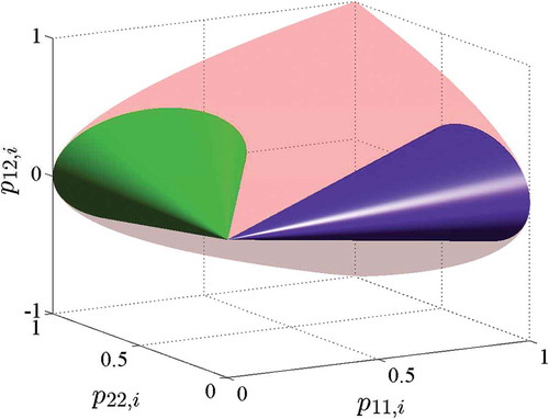
The convex cones ${\mathcal{P}}_1,{\mathcal{P}}_2,{\mathcal{C}}_1,{\mathcal{C}}_2$ are illustrated in Figure 1 and the axes show the entries of the matrices ${\mathbf{P}}_i$. Consider the objective function (Equations (26) and (28))

(31) $\begin{array}{cc}{J}_{\mathbf{W},i}=\parallel {\mathbf{P}}_i-{\mathbf{I}}_2{\parallel }_F^2& =\mathrm{t}\mathrm{r}({\mathbf{P}}_i{\mathbf{P}}_i)-2\mathrm{t}\mathrm{r}({\mathbf{P}}_i)+\mathrm{t}\mathrm{r}({\mathbf{I}}_2)\\ \hspace{0.17em}& =(p_{11,i}-{1)}^2+{(p_{22,i}-1)}^2+2p_{12,i}^2.\end{array}$(31)

Figure 1. Convex cones ${\mathcal{C}}_1$ (left), ${\mathcal{C}}_2$ (right) and ${\mathcal{P}}_1,{\mathcal{P}}_2$.

Then, STABLE minimizes the objective function $J_{\mathbf{W},i}$ so that the optimal solution ${\mathbf{P}}_i^{\ast }$ is an element of the respective convex cone ${\mathcal{C}}_i$:

(32) ${\mathbf{P}}_1^{\ast }=\left[\begin{array}{cc}0.745& 0\\ 0& 1.164\end{array}\right],{\mathbf{P}}_2^{\ast }=\left[\begin{array}{cc}1.164& 0\\ 0& 0.745\end{array}\right].$(32)

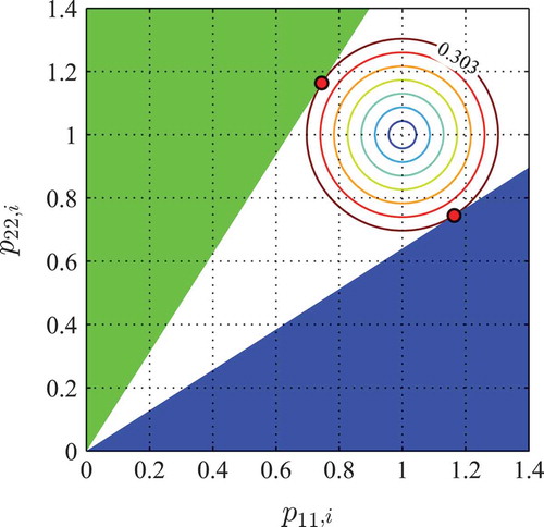
For solving the convex program STABLE, the package CVX is used [32,33]. The results are obtained using solver SeDuMi [37]. Operating on a 2.20-GHz processor, solving the semidefinite programs lasted ${\bar{t}}_{\mathrm{S}\mathrm{T}\mathrm{A}\mathrm{B}\mathrm{L}\mathrm{E}}=0.5$s on average for each of the two grid points. A graphical interpretation of the optimization problem is given in Figure 2. The axes show the entries $p_{11,i},p_{22,i}$ of the matrices ${\mathbf{P}}_i$ for $p_{12,i}=0$. The objective functions $J_{\mathbf{W},i}$ from Equation (31) describe circles in the plane $p_{12,i}=0$ with midpoint $(p_{11,i},p_{22,i})=(1,1)$ and radius $\sqrt{J_{\mathbf{W},i}}$. The convex cones ${\mathcal{C}}_1,{\mathcal{C}}_2$ are shown as triangles which are the intersection of the convex cones from Figure 1 with the plane $p_{12,i}=0$. The algorithm STABLE searches for the solutions $(p_{11,i}^{\ast },p_{22,i}^{\ast })$ with the minimum value of the objective functions $J_{\mathbf{W},i}$ so that the solutions lie in the convex cones ${\mathcal{C}}_1,{\mathcal{C}}_2$. This is the case for the solutions (Equation (32)) which are the points where the circle with radius $\sqrt{J_{\mathbf{W},i}}=0.303$ touches the cones. This results in the transformation matrices ${\mathbf{M}}_i={\mathbf{P}}_i^{\ast }$ which lead to the reduced systems $P_i^{*}{\dot{\tilde{x}}}_i(t)=P_i^{*}{\widehat{A}}_i{\tilde{x}}_i(t)$. Then, the interpolated reduced system is $\tilde{E}(p)\dot{\tilde{x}}(t,p)=\tilde{A}(p)\tilde{x}(t,p)$ with $\tilde{\mathbf{E}}(p)={\sum }_{i=1}^2{\omega }_i(p){\mathbf{P}}_i^{\ast }$ and $\tilde{\mathbf{A}}(p)={\sum }_{i=1}^2{\omega }_i(p){\mathbf{P}}_i^{\ast }{\hat{\mathbf{A}}}_i$ with linear weighting functions ${\omega }_i(p)$. The interpolated system possesses the Lyapunov function $V(\tilde{x}(t,p))=\tilde{x}(t,p{)}^T(\sum _{i=1}^2{\omega }_i(p){\mathbf{P}}_i^{\ast })\tilde{x}(t,p)$ and hence is asymptotically stable for the entire domain $\mathcal{D}$. The price paid is an increase of the minimum value of the objective functions $J_{\mathbf{W},i}({\mathbf{P}}_i^{\ast })$ since the left ROBs are distorted as little as possible to ${\tilde{\mathbf{W}}}_i={\mathbf{W}}_0{\mathbf{P}}_i^{\ast }$ (see Table 1).

Table 1. Comparison of the adjusted ROBs and of the respective minimum values of the objective functions for matrix interpolation with and without STABLE.

	Without STABLE	With STABLE
ROBs	${\tilde{\mathbf{V}}}_i^{\mathrm{W}\mathrm{S}}={\mathbf{V}}_0$	${\tilde{\mathbf{V}}}_i={\mathbf{V}}_0$
	${\tilde{\mathbf{W}}}_i^{\mathrm{W}\mathrm{S}}={\mathbf{W}}_0$	${\tilde{\mathbf{W}}}_i={\mathbf{W}}_0{\mathbf{P}}_i^{\ast }$
Objective functions	$J_{\mathbf{V},i}^{\mathrm{W}\mathrm{S}}({\mathbf{I}}_2)=0$	$J_{\mathbf{V},i}({\mathbf{I}}_2)=0$
	$J_{\mathbf{W},i}^{\mathrm{W}\mathrm{S}}({\mathbf{I}}_2)=0$	$J_{\mathbf{W},i}({\mathbf{P}}_i^{\ast })={0.303}^2$

Figure 2. Convex cones ${\mathcal{C}}_1$ (top left), ${\mathcal{C}}_2$ (bottom right) in the plane $p_{12,i}=0$ and optimal $(p_{11,i}^{\ast },p_{22,i}^{\ast })$ with minimum cost function $J_{\mathbf{W},i}={0.303}^2$.

5.2. Anemometer

The anemometer is a flow sensing device [38,39]. It consists of a heater and two temperature sensors that are located before and after the heater. If there is no flow, the heat dissipates symmetrically into the fluid. This symmetry is disturbed if a flow is applied to the fluid, which leads to convection of the temperature field. Then, the fluid velocity can be determined from the difference between the temperatures measured with the sensors. The governing equation is the convection-diffusion partial differential equation

(33) $\rho c_p\frac{\mathrm{\partial }T}{\mathrm{\partial }t}=\mathrm{\nabla }(\kappa \mathrm{\nabla }T)-\rho c_{p}v\mathrm{\nabla }T+\dot{Q},$(33)

where $\rho$ denotes the mass density, $c_p=0.5\mathrm{J}\mathrm{k}{\mathrm{g}}^{-1}{\mathrm{K}}^{-1}$ is the specific heat, $T$ is the temperature and $\dot{Q}$ is the heat flow into the system caused by the heater. The thermal conductivity varies in $\kappa \in [1,2]\mathrm{W}{\mathrm{m}}^{-1}{\mathrm{K}}^{-1}$ and the fluid velocity in $v\in [0.1,2]\mathrm{m}{\mathrm{s}}^{-1}$. Finite element discretization of the convection-diffusion Equation (33), with zero Dirichlet boundary conditions, leads to the parameter-dependent state-space system of order $n=29008$

(34) $\begin{array}{cc}\mathbf{E}\dot{\mathbf{T}}(t,\kappa ,v)& =\stackrel{\mathbf{A}(\kappa ,v)}{\overbrace{({\mathbf{A}}_0+\kappa {\mathbf{A}}_1+v{\mathbf{A}}_2)}}\mathbf{T}(t,\kappa ,v)+\mathbf{b}\dot{Q}(t)\\ y(t,\kappa ,v)& ={\mathbf{c}}^T\mathbf{T}(t,\kappa ,v),\end{array}$(34)

where $\mathbf{T}(t,\kappa ,v)\in {\mathbb{R}}^{29008}$ is the state vector, containing the temperatures at the discretization nodes. The input is the heat source $\dot{Q}(t)$ and the output is the temperature difference between the sensors. The parameter vector is $p=[v\kappa {]}^T$ and the parameter domain is normalized to $\mathcal{D}=[0,1]\times [0,1]$. For the sake of simplicity, the domain is sampled for the set of points of an equidistant grid $\mathcal{P}=\{0,1/5,\dots ,1\}\times \{0,1/5,\dots ,1\}$, which result in the set of $N=36$ high-order systems $\mathcal{G}=\{{\mathbf{G}}_1,\dots ,{\mathbf{G}}_{36}\}$. The local systems are reduced to order $q=10$ using IRKA, which result in a set of asymptotically stable reduced systems $\hat{\mathcal{G}}=\{{\hat{\mathbf{G}}}_1,\dots ,{\hat{\mathbf{G}}}_{36}\}$ according to Equation (4). For testing the systems $\hat{\mathcal{G}}$, we compute the error in ${\mathcal{H}}_{\mathrm{\infty }}$-norm at the points of the grid $\mathcal{P}$ using the formula

(35) $e_{{\mathcal{H}}_{\mathrm{\infty }}}(p)=\frac{||\mathbf{G}(p)-\hat{\mathbf{G}}(p{)||}_{{\mathcal{H}}_{\mathrm{\infty }}}}{||\mathbf{G}(p{)||}_{{\mathcal{H}}_{\mathrm{\infty }}}}\approx \frac{\underset{1\le k\le K}{\mathrm{m}\mathrm{a}\mathrm{x}}{\sigma }_{\mathrm{m}\mathrm{a}\mathrm{x}}\{\mathbf{G}(j{\omega }_k,p)-\hat{\mathbf{G}}(j{\omega }_k,p)\}}{\underset{1\le k\le K}{\mathrm{m}\mathrm{a}\mathrm{x}}{\sigma }_{\mathrm{m}\mathrm{a}\mathrm{x}}\{\mathbf{G}(j{\omega }_k,p)\}},$(35)

where ${\sigma }_{\mathrm{m}\mathrm{a}\mathrm{x}}$ is the largest singular value and $j=\sqrt{-1}$. For approximating this error, we choose $K=50$ equally spaced frequencies ${\omega }_1,{\omega }_2,\dots ,{\omega }_K$ in the frequency range of interest $[{10}^1,\dots ,{10}^6]$ and we obtain the error $e_{{\mathcal{H}}_{\mathrm{\infty }}}^{\mathcal{P}}:\mathcal{P}\to {\mathbb{R}}_0^{+}$ with $e_{{\mathcal{H}}_{\mathrm{\infty }}}^{\mathcal{P}}\in [3.6\cdot {10}^{-5},3.0\cdot {10}^{-4}]$. We calculate the reference basis ${\mathbf{V}}_0$ using the non-weighted SVD approach (Equation (6)) and the reference basis ${\mathbf{W}}_0$ is determined in the dual way.

5.2.1. Matrix interpolation without using STABLE

Firstly, the interpolation procedure will be demonstrated without the stability-preserving method, which corresponds to the framework from Section 2.4. The respective values are labelled with WS. The transformation matrices for adjusting the right ROBs are calculated using the MAC or DS approach minimizing the objective function (Equation (7) or (8)) which results in ${\mathbf{T}}_{\mathrm{M}\mathrm{A}\mathrm{C},i}^{\mathrm{W}\mathrm{S}}=({\mathbf{V}}_0^T{\mathbf{V}}_i{)}^{-1}$ or ${\mathbf{T}}_{\mathrm{D}\mathrm{S},i}^{\mathrm{W}\mathrm{S}}={\mathbf{V}}_i^{+}{\mathbf{V}}_0$ for $i\in \{1\dots ,36\}$. For adjusting the left ROBs, we obtain ${\mathbf{M}}_{\mathrm{M}\mathrm{A}\mathrm{C},i}^{\mathrm{W}\mathrm{S}}=({\mathbf{W}}_0^T{\mathbf{W}}_i{)}^{-1}$ or ${\mathbf{M}}_{\mathrm{D}\mathrm{S},i}^{\mathrm{W}\mathrm{S}}={\mathbf{W}}_i^{+}{\mathbf{W}}_0$ using the MAC or DS approach minimizing the objective function (Equation (9) or (10)). The local systems are transformed according to Equation (11) and result in the systems ${\tilde{\mathcal{G}}}^{\mathrm{W}\mathrm{S}}=\{{\tilde{\mathbf{G}}}_1^{\mathrm{W}\mathrm{S}},\dots ,{\tilde{\mathbf{G}}}_{36}^{\mathrm{W}\mathrm{S}}\}$. The parametric reduced system ${\tilde{\mathbf{G}}}^{\mathrm{W}\mathrm{S}}(p)$ is obtained by interpolating the systems of the set ${\tilde{\mathcal{G}}}^{\mathrm{W}\mathrm{S}}$ according to Equations (12) and (13) using bilinear weighting functions. For testing the system, we compute the error in ${\mathcal{H}}_{\mathrm{\infty }}$-norm at the points of a test grid ${\mathcal{P}}_{\mathrm{t}\mathrm{e}\mathrm{s}\mathrm{t}}=\{0,1/80,\dots ,1\}\times \{0,1/80,\dots ,1\}$ according to Equation (35). 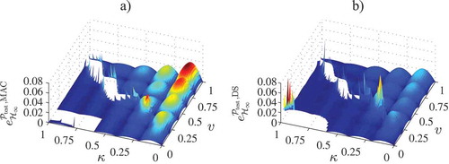In Figure 3, the error $e_{{\mathscr{H}}_{\infty }}^{}:{}_{\text{test}}\to {ℝ}_0^{+}$ is plotted for both quality functions. The reader can verify that there are regions in the domain – where the ${\mathcal{H}}_{\mathrm{\infty }}$-norm equals infinity – which exhibit instability of the interpolation procedure.

Figure 3. Error $e_{{\mathcal{H}}_{\mathrm{\infty }}}^{{\mathcal{P}}_{\mathrm{t}\mathrm{e}\mathrm{s}\mathrm{t}}}$ without the stability-preserving method and the (a) MAC approach and the (b) DS approach.

5.2.2. Matrix interpolation using STABLE

Secondly, the proposed stability-preserving method is applied. The transformation matrices for adjusting the right ROBs are ${\mathbf{T}}_i={\mathbf{T}}_i^{\mathrm{W}\mathrm{S}}$ for $i\in \{1\dots ,36\}$ for the MAC and DS approaches minimizing the objective function (Equation (7) or (8)). For adjusting the left ROBs, we calculate the transformation matrices ${\mathbf{M}}_1,\dots ,{\mathbf{M}}_{36}$ using STABLE with the MAC and DS approach. For specifying and solving the convex program STABLE, the package CVX is used [32,33]. The results are obtained using solver SeDuMi [37] and verified with SDPT3 [40]. Operating on a 2.20GHz processor, solving the semidefinite programs lasted ${\bar{t}}_{\mathrm{S}\mathrm{T}\mathrm{A}\mathrm{B}\mathrm{L}\mathrm{E}}=1$s on average for each of the $N=36$ grid points. The local systems of the set $\hat{\mathcal{G}}$ are transformed according to Equation (11) and result in the systems $\tilde{\mathcal{G}}=\{{\tilde{\mathbf{G}}}_1,\dots ,{\tilde{\mathbf{G}}}_{36}\}$. 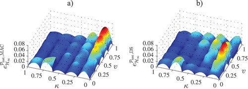The parametric reduced system $\tilde{\mathbf{G}}(p)$ is obtained by interpolating the systems of the set $\tilde{\mathcal{G}}$ according to Equations (12) and (13) using bilinear weighting functions. The error $e_{{\mathcal{H}}_{\mathrm{\infty }}}^{{\mathcal{P}}_{test}}:{\mathcal{P}}_{test}\to {\mathbb{R}}_0^{+}$ according to Equation (35) of the reduced system $\tilde{\mathbf{G}}(p)$ is shown in Figure 4 for the MAC approach and the DS approach. The MAC approach leads to the mean error ${\bar{e}}_{{\mathcal{H}}_{\mathrm{\infty }}}^{{\mathcal{P}}_{\mathrm{t}\mathrm{e}\mathrm{s}\mathrm{t}},\mathrm{M}\mathrm{A}\mathrm{C}}=0.016$ and the maximum error $e_{{\mathcal{H}}_{\mathrm{\infty }},\mathrm{m}\mathrm{a}\mathrm{x}}^{{\mathcal{P}}_{\mathrm{t}\mathrm{e}\mathrm{s}\mathrm{t}},\mathrm{M}\mathrm{A}\mathrm{C}}=0.070$. The DS approach has the mean error ${\bar{e}}_{{\mathcal{H}}_{\mathrm{\infty }}}^{{\mathcal{P}}_{\mathrm{t}\mathrm{e}\mathrm{s}\mathrm{t}},\mathrm{D}\mathrm{S}}=0.017$ and the maximum error $e_{{\mathcal{H}}_{\mathrm{\infty }},\mathrm{m}\mathrm{a}\mathrm{x}}^{{\mathcal{P}}_{\mathrm{t}\mathrm{e}\mathrm{s}\mathrm{t}},\mathrm{D}\mathrm{S}}=0.071$. The reader can verify that the proposed method preserves the stability of the interpolated system for the entire domain $\mathcal{D}$. In addition, the method delivers nearly as accurate results as the method without stability preservation – compared for regions where the latter is asymptotically stable – since the left ROBs are distorted as little as possible.

Figure 4. Error $e_{{\mathcal{H}}_{\mathrm{\infty }}}^{{\mathcal{P}}_{test}}$ using STABLE and the (a) MAC approach and (b) DS approach.

6. Conclusions

In this article, a method for pMOR by matrix interpolation with stability preservation is presented. This approach makes neither demands on the structure of the original system nor needs post-processing during the online phase to achieve stability and therefore is suitable for real-time applications. The procedure is based on low-order convex optimization problems – so-called semidefinite programs – which can easily be implemented and solved.

Disclosure statement

No potential conflict of interest was reported by the authors.

Notes

1. The matrix 0_n×n of size n × n contains only zeros. The matrix In is the identity matrix of size n. Symmetric matrices of size n are denoted by $\mathbf{Q}\in {\mathbb{S}}_n$. Symmetric positive definite matrices of size n are denoted by $\mathbf{Q}\in {\mathbb{S}}_n^{++}$ or $\mathbf{Q}>{\mathbf{0}}_{n\times n}$. Symmetric negative definite matrices of size n are denoted by $\mathbf{Q}<{\mathbf{0}}_{n\times n}$.

References

- A.C. Antoulas, Approximation of Large-Scale Dynamical Systems, SIAM, Philadelphia, 2005.
- S. Grivet-Talocia, Black-box passive macromodeling in electronics: trends and open problems, in ECMI Newsletter, Number 56, European Consortium for Mathematics in Industry, Helsinki, 2014, pp. 40–43.
- S. Gugercin, R.V. Polyuga, C. Beattie, and A. Van Der Schaft, Structure-preserving tangential interpolation for model reduction of Port-Hamiltonian systems, Automatica 48 (9) (2012), pp. 1963–1974. doi:10.1016/j.automatica.2012.05.052
- P. Benner, S. Gugercin, and K. Willcox, A survey of projection-based model reduction methods for parametric dynamical systems, SIAM Rev. 57 (4) (2015), pp. 483–531. doi:10.1137/130932715
- D. Amsallem and C. Farhat, An online method for interpolating linear parametric reduced-order models, SIAM J. Sci. Comput. 33 (5) (2011), pp. 2169–2198. doi:10.1137/100813051
- J. Degroote, J. Vierendeels, and K. Willcox, Interpolation among reduced-order matrices to obtain parameterized models for design, optimization and probabilistic analysis, Int. J. Numer. Methods Fluids 63 (2) (2010), pp. 207–230.
- M. Geuss. A Black-box method for parametric model order reduction based on matrix interpolation with application to simulation and control, PhD thesis, submitted, TU München, 2015.
- M. Geuss, H. Panzer, and B. Lohmann, On parametric model order reduction by matrix interpolation, Proceedings of the European Control Conference, Zurich, Switzerland, 2013, pp. 3433–3438.
- B. Lohmann and R. Eid, Efficient order reduction of parametric and nonlinear models by superposition of locally reduced models, in Methoden und Anwendungen der Regelungstechnik. Erlangen-Münchener Workshops 2007 und 2008, B. Lohmann and G. Roppenecker, eds., Shaker-Verlag, Aachen, 2009, pp. 1–20.
- H. Panzer, J. Mohring, R. Eid, and B. Lohmann, Parametric model order reduction by matrix interpolation, at-Automatisierungstechnik 58 (8) (2010), pp. 475–484. doi:10.1524/auto.2010.0863
- R. Eid, R. Castañé-Selga, H. Panzer, T. Wolf, and B. Lohmann, Stability-preserving parametric model reduction by matrix interpolation, Math. Comput. Model. Dyn. Syst. 17 (4) (2011), pp. 319–335. doi:10.1080/13873954.2011.547671
- M. Giftthaler, T. Wolf, and H. Panzer, Parametric model order reduction of Port-Hamiltonian systems by matrix interpolation, at-Automatisierungstechnik 62 (9) (2014), pp. 619–628. doi:10.1515/auto-2013-1072
- O. Farle, S. Burgard, and R. Dyczij-Edlinger, Passivity preserving parametric model-order reduction for non-affine parameters, Math. Comput. Model. Dyn. Syst. 17 (3) (2011), pp. 279–294. doi:10.1080/13873954.2011.562901
- F. Ferranti, G. Antonini, T. Dhaene, and L. Knockaert, Guaranteed passive parameterized model order reduction of the Partial Element Equivalent Circuit (PEEC) method, IEEE Trans. Electromagn. Compat. 52 (4) (2010), pp. 974–984. doi:10.1109/TEMC.2010.2051949
- L. Knockaert, T. Dhaene, F. Ferranti, and D. De Zutter, Model order reduction with preservation of passivity, non-expansivity and markov moments, Syst. Control. Lett. 60 (1) (2011), pp. 53–61. doi:10.1016/j.sysconle.2010.10.006
- E.R. Samuel, F. Ferranti, L. Knockaert, and T. Dhaene, Passivity-preserving parameterized model order reduction using singular values and matrix interpolation, IEEE Trans. Compon. Packag. Manuf. Technol. 3 (6) (2013), pp. 1028–1037. doi:10.1109/TCPMT.2013.2248196
- B.N. Bond and L. Daniel, Stable reduced models for nonlinear descriptor systems through piecewise-linear approximation and projection, IEEE Trans. Computer-Aided Des. Integr. Circuits Syst. 28 (10) (2009), pp. 1467–1480. doi:10.1109/TCAD.2009.2030596
- M. Geuss, H. Panzer, T. Wolf, and B. Lohmann, Stability preservation for parametric model order reduction by matrix interpolation, Proceedings of the European Control Conference, Strasbourg, France, 2014, pp. 1098–1103.
- T. Kailath, Linear Systems, Prentice Hall, Englewood Cliffs, 1980.
- H.K. Khalil, Nonlinear Systems, 3rd ed., Prentice Hall, Upper Saddle River, NJ, 2002.
- T. Stykel, Analysis and numerical solution of generalized Lyapunov equations, PhD thesis, TU Berlin, 2002.
- H. Panzer, B. Kleinherne, and B. Lohmann, Analysis, Interpretation and generalization of a strictly dissipative state space formulation of second order systems, in Methoden und Anwendungen der Regelungstechnik. Erlangen-Münchener Workshops 2011 und 2012, B. Lohmann and G. Roppenecker, eds., Shaker-Verlag, Aachen, 2013, pp. 59–75.
- R. Castañé-Selga, B. Lohmann, and R. Eid, Stability preservation in projection-based model order reduction of large scale systems, Eur. J. Control 18 (2) (2012), pp. 122–132. doi:10.3166/ejc.18.122-132
- M. Geuss, H. Panzer, I. Clifford, and B. Lohmann, Parametric model order reduction using pseudoinverses for the matrix interpolation of differently sized reduced models, Proceedings of the 19th IFAC World Congress, Cape Town, South Africa, 2014, pp. 9468–9473.
- H. Panzer, S. Jaensch, T. Wolf, and B. Lohmann, A greedy rational Krylov method for μ2-pseudooptimal model order reduction with preservation of stability. Proceedings of the American Control Conference, Washington, DC, 2013, pp. 5512–5517.
- S. Gugercin, A.C. Antoulas, and C. Beattie, μ2 model reduction for large-scale linear dynamical systems, SIAM J. Matrix Anal. Appl. 30 (2) (2008), pp. 609–638. doi:10.1137/060666123
- D. Amsallem and C. Farhat, Stabilization of projection-based reduced-order models, Int. J. Numer. Methods Eng. 91 (4) (2012), pp. 358–377. doi:10.1002/nme.v91.4
- B.N. Bond and L. Daniel, Guaranteed stable projection-based model reduction for indefinite and unstable linear systems, Proceedings of the IEEE/ACM International Conference on Computer-Aided Design, San Jose, CA, 2008, pp. 728–735.
- L. Vandenberghe and S. Boyd, Semidefinite programming, SIAM Rev. 38 (1) (1996), pp. 49–95. doi:10.1137/1038003
- S. Boyd and L. Vandenberghe, Convex Optimization, Cambridge University Press, New York, NY, 2004.
- S. Boyd, L. El Ghaoui, E. Feron, and V. Balakrishnan, Linear matrix inequalities in system and control theory, in Studies in Applied Mathematics, SIAM, Philadelphia, PA, 1994.
- M. Grant and S. Boyd, CVX: MATLAB software for disciplined convex programming, version 2.0, Aug, 2012. Available at http://cvxr.com/cvx.
- M. Grant and S. Boyd, Graph implementations for nonsmooth convex programs, in Recent Advances in Learning and Control, Lecture Notes in Control and Information Sciences, V. Blondel, S. Boyd, and H. Kimura, eds., Springer, London, 2008, pp. 95–110.
- Y. Nesterov and A. Nemirovskii, Interior-point polynomial algorithms in convex programming, in Studies in Applied Mathematics, SIAM, Philadelphia, PA, 1994.
- M.J. Todd, Semidefinite optimization, Acta Numer. 10 (2001), pp. 515–560. doi:10.1017/S0962492901000071
- L. Vandenberghe and S. Boyd, A polynomial-time algorithm for determining quadratic Lyapunov functions for nonlinear systems. Proceedings of the European Conference Circuit Theory Design, Davos, Switzerland, 1993, pp. 1065–1068.
- J.F. Sturm, Using SeDuMi 1.02, a MATLAB toolbox for optimization over symmetric cones, Optim. Methods Softw. 11 (1999), pp. 625–653. doi:10.1080/10556789908805766
- MOR Wiki. Available at http://www.modelreduction.org.
- C. Moosmann, E.B. Rudnyi, A. Greiner, J.G. Korvink, and M. Hornung, Parameter preserving model order reduction of a flow meter. Proceedings of the NSTI Nanotech, 3, Anaheim, CA, 2005, pp. 684–687.
- R.H. Tütüncü, K.C. Toh, and M.J. Todd, Solving semidefinite-quadratic-linear programs using SDPT3, Math. Programming Ser. B 95 (2003), pp. 189–217. doi:10.1007/s10107-002-0347-5