Interface and model reduction for efficient explicit simulations - a case study with nonlinear vehicle crash models

ABSTRACT

This work presents an approach to save simulation time in explicit crash simulations of vehicles by applying model order reduction (MOR). The model of a kart frame is split into linear and nonlinear parts. The linear part is reduced with linear MOR techniques in MatMorembs. Optimal substructuring methods are used to calculate suitable reduced models which are exported to LS-DYNA. Afterwards, the model consisting of a linear reduced part and a nonlinear part is simulated in the online step. The plastic deformation of the kart frame as well as the accelerations of the driver calculated with various reduction and parameter settings are compared with the accelerations measured when the original, unreduced nonlinear model is simulated. For optimal simulation results, the large interface between the models needs to be approximated by suitable interface-reduction approaches. The novel contribution is the application of advanced interface-reduction techniques in nonlinear explicit crash simulations. Craig–Bampton and Gramian matrix-based-like techniques with global, local and no interface reduction are compared to find optimally reduced substructures in terms of approximation quality of the assembled system and computational effort. For the kart frame, the applicability of the method is proven by gaining a small simulation speed up which cannot be achieved with the standard reduction methods provided by LS-DYNA.

KEYWORDS:

• Explicit crash simulation
• model order reduction
• interface reduction
• nonlinear FEM

1. Introduction

Numerical simulation is accepted as the third pillar of scientific inquiring, alongside theory and experiment. The virtual product development process, called Digital Mockup, of many technical systems, e.g. the development of planes, cars, trains, robots, chip design, prostheses, etc. relies heavily on simulation results, see e.g. [1–3]. Simulations are made to derive control strategies, evaluate the performance of a technical system before a prototype is available and perform optimizations [4]. In this contribution, a closer look is taken at simulations within an explicit finite element (FE) code like LS-DYNA. Explicit nonlinear FE programmes are especially well suited to analyse short-term transient dynamical processes. One of the main applications of nonlinear FE programmes is the simulation of vehicle crashes in order to improve passenger safety in automotive design. Even before a first prototype is produced, many virtual crashes are performed to find designs which make the car safer. Crash simulation is one of the most time-consuming tasks in computer-aided automotive design. In order to allow for parallelization on computer clusters, explicit instead of implicit methods are used to solve the occurring differential equations in crash simulation. This already reduces the response time, time until the simulation is finished and the analysis of the results can start, but not the overall computational cost. Therefore, the deployment of methods for speed-up, data reduction and energy saving in the computing centres is a logical consequence. Various approaches exist to speed up explicit finite element codes, e.g. selective mass scaling [5], domain composition method [6] or the usage of implicit integration schemes. These methods aim to decrease simulation time by increasing the bounded maximal stable time step size Δt. The current status of subcycling and selective mass scaling with LS-DYNA, one of the big commercial codes, is given for example by [7].

Another possibility to speed up simulations is the reduction of the degrees of freedom by model order reduction (MOR). The main idea of MOR is the approximation of a large-scale dynamical system, e.g. the nonlinear ordinary differential equations (ODE) system of an FE model of dimension N with a system of much smaller dimension n where the most dominant features of the large-scale system like input–output behaviour, passivity, stability, etc. are retained in the small-scale system as precisely as possible. The generation of the reduced model is mostly performed once in a so-called offline phase, which might be computationally expensive. Then, the reduced model can be simulated rapidly and possibly repeatedly during the so-called online phase. In general, we distinguish between linear and nonlinear reduction methods, see e.g. [8–10] for an overview of methods, application areas as well as evolving problems in linear reduction methods and [11] for nonlinear reduction methods.

In a crash scenario, some parts of the automobile exhibit large deformations and nonlinear behaviour, whereas others experience merely small linear vibrations [12]. Therefore, we suggest a new approach to speed up crash simulations. The workflow of our approach is depicted in Figure 1.

Figure 1. Workflow of the process suggested to speed up explicit simulations. The new converters and procedures derived in the course of this research are the Binout-Reader, the LS-Dyna import and the d3eigv writer. Furthermore, the workflow shows how MatMorembs is used to calculate the reduced elastic body for the online simulation.

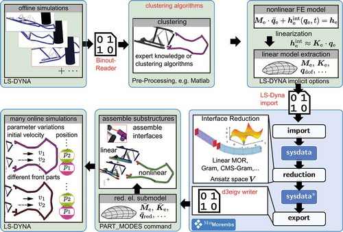
Using linear reduction for a nonlinear part would result in a large error. Furthermore, it is unnecessary and computationally too expensive to reduce the complete model with nonlinear techniques. Therefore, parts with linear and nonlinear characteristics are identified in a first step. In order to determine which parts of the model exhibit small deformations and can be described with a linear model, it is necessary to run multiple simulations with varying parameters, e.g. impact velocity in an offline step (see Figure 1, the upper left part). As it is always considered in offline/online scenarios, the time savings in the multiquery online simulations with the reduced models are large enough to justify the considerable amount of time spent in the offline step. The variations in the offline step must include the scenarios which are considered in the successive analyses. Afterwards, the identification of linear and nonlinear behaviour (Figure 1 upper middle part) could either be performed by an experienced user or by the application of methods from machine learning, cf. [13] and [14]. For the identification of the nonlinear and linear components in Matlab, we developed a converter binout-reader to have direct access to the LS-DYNA binary files. Now it is possible to substructure the model into nonlinear and into linear parts. The usage of nonlinear reduction techniques like hyper-reduction [15] or the energy-conserving sampling and weighting (ECSW) hyper-reduction [16] are very code intrusive and therefore require specialized FE routines which are not yet available in commercial FE programmes. Therefore, we focus on the linear part which should be approximated by linear ansatz functions in this preliminary work. So far, MOR is sparely used for crashes. Usually only traditional linear modal forms are used, e.g. the component mode synthesis (CMS) method, if at all. However, as mentioned in [17,18], reduction methods other than CMS exist for reduction of coupled FE problems, which can lead to better reduction results. Therefore, instead of using the internal LS-DYNA capabilities for MOR, we extract in a first step the system matrices via clustering separated parts. Accordingly, the nonlinear FE model is linearized by using the implicit options and exporting the linear system matrices. Afterwards, a converter was developed to import the linearized LS-DYNA model in the MOR programme MatMorembs [19]. As a consequence, all the non-modal and additional features of MatMorembs are now available and can be used to calculate an optimal ansatz space. Another topic mentioned and explained in this article is the correct modelling and handling of the interfaces between the linearly approximated and nonlinear parts, see e.g. [18], which is critical for good reduction results. In this article, the interface-reduction approach of [18] is applied in explicit crash simulations and in a coupling scenario between linear and nonlinear models for the first time. Subsequent to the interface reduction, we calculate the most suitable ansatz functions to approximate the rear part. Afterwards, the linearized reduced model is exported via a newly written d3eigv-writer towards LS-DYNA (see Figure 1 lower right part). LS-DYNA assembles a reduced elastic body with the *PART_MODES command, see e.g. [20].

Finally, the reduced model consisting of a linear reduced part and a nonlinear part is simulated with LS-DYNA in the online step. This can be used to perform many optimization or parametric runs (see Figure 1 lower left part).

To concentrate on the essential questions, all studies are performed with a simple racing kart depicted in Figure 2 and Figure 3. The racing kart is a simple automobile. Hence, its dynamical behaviour is strongly influenced by the deformation and vibration characteristics of the frame.

Figure 2. Race kart used as a simple surrogate vehicle model. The race kart consists of a frame, an engine next to the seat, a rear shaft, frontal steering components and tyres.

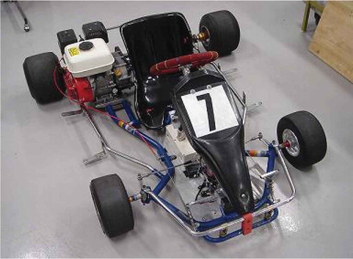
Figure 3. Main parts of the simulated crash scenario. The kart frame crashes into the rigid pole. Forces and moments represent the interactions between kart frame, tyres and rear shaft.

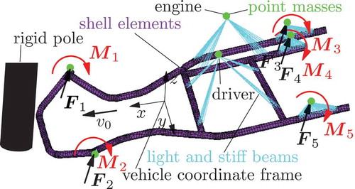
The kart frame crashes into a rigid pole with the velocity v₀, see Figure 3. The crash behaviour is strongly influenced by the nonlinear plastic deformation characteristics of the frame. Therefore, the kart frame is an ideal example to discuss the performance of various MOR methods for structures in crashes. The frontal section experiences a strong nonlinear plastic deformation whereas the rear section only exhibits vibrations of small amplitude. As a consequence, an approximation with a linear model is suitable for the rear part. Several reduction techniques to reduce the number of interface degrees of freedom (DOF) and elastic DOF are compared regarding quality and computational effort.

Section 2 of the paper gives a brief theoretical overview of the topics involved in this research. In Section 3, a more detailed explanation of the example and the offline step necessary to partition the model into linear and nonlinear parts is given. We present results regarding the approximation quality in Section 4 and conclude this paper in Section 5 with a summary and outlook on future work.

2. Theoretical background

First, a description of the necessary theoretical background is given, subdivided into the different relevant fields.

2.1. Crash simulation

Crash simulations possess three basic sources of nonlinearities in mechanics: geometrical nonlinearities that arise in large deformation problems like large rotations, large strains and large displacements; nonlinear material behaviour and the nonlinear behaviour of multiple contact scenarios. Therefore, nonlinear explicit FE solvers based on an updated Lagrangian formulation, see e.g. [21,22] are used to simulate the highly dynamic crash event.

The nonlinear FE method is a systematic approach to transform the fundamental laws of continuum mechanics of a solid from a set of partial differential equations (PDE) into a large set of ODE by discretization of the problem with respect to space and time. For solids, the displacement of a point of the continuum is, for instance, approximated by r (x, t) = Φ (x) q_e (t), where the columns of Φ (x) define a global space-dependent basis of ansatz functions and ${\mathbf{q}}_{\mathrm{e}}(t)\in {\mathbb{R}}^N$ is a time-dependent vector of nodal DOFs. With such a discretization in space, a solid in a crash event is described by a system of ordinary differential equations with respect to time and reads

(1) $M_{\text{e}}\cdot {\stackrel{\mathrm{..}}{q}}_{\text{e}}+h_{\text{e}}^{\text{int}}(q_{\text{e}},t)=h_{\text{e}}$(1)

with the symmetric mass matrix $M_{\mathrm{e}}\in {\mathbb{R}}^{N\times N}$, the elastic stiffness vector $h_{\mathrm{e}}^{\mathrm{i}\mathrm{n}\mathrm{t}}(q_{\mathrm{e}},t)\in {\mathbb{R}}^N$ and the applied forces $h_{\mathrm{e}}\in {\mathbb{R}}^N$. By adding suitable initial conditions, an initial-value problem is formed. Nowadays, FE models for the simulation of a crash event can have more than N > 10⁷ DOFs. For the integration of the nonlinear differential equation, efficient integration schemes are necessary to evolve from the initial time t₀ to the end time T in K time steps. Crash simulations use explicit integration schemes more than implicit schemes because they can be parallelized easily and are especially well suited for transient analysis over a short time period. One important feature of explicit FE solutions is the fact that most of the calculations are made on the element level, and, therefore, explicit calculations are especially well suited for distributed computation systems. One of the most time-consuming parts of the integration procedure is the calculation of the internal and external forces on the element level in every time step k.

The calculation of the internal forces $h_{\mathrm{e}}^{\mathrm{i}\mathrm{n}\mathrm{t}}$ depends on the constitutive laws, which describe how stresses at the continuum relate to the strain e, the strain rate ė, load history, etc. Different constitutive laws are used depending on the material used, the grade of expected deformation and the analyses performed. In general, the internal forces $h_{\mathrm{e}}^{\mathrm{i}\mathrm{n}\mathrm{t}}=h_{\mathrm{e}}^{\mathrm{i}\mathrm{n}\mathrm{t}}(q_{\mathrm{e}}(t),\dots )$ are a nonlinear function of the nodal displacements, nodal velocities and other variables. Under considerations, such as small displacements and linear-elastic material laws, a linear FE approach is admissible. In a linear FE approach, the internal forces can be calculated by $h_{\mathrm{e}}^{\mathrm{i}\mathrm{n}\mathrm{t}}=K_{\mathrm{e}}\cdot q_{\mathrm{e}}$ with the symmetric and at least positive semidefinite linear stiffness matrix K_e which is assembled once and is constant for the whole simulation. In the presented simulation scenario, the rear part of the kart is well approximated by a linearly reduced FE model. Therefore, it is necessary to linearize the nonlinear FE Equation (1) around a suitable working point with the help of the implicit solver option of LS-DYNA to a linear FE system

(2) $M_{\text{e}}\cdot {\stackrel{\mathrm{..}}{q}}_{\text{e}}(t)+K_{\text{e}}\cdot q_{\text{e}}(t)=h_{\text{e}}(t)$(2)

(3) $h_{\mathrm{e}}(t)\in {\mathbb{R}}^N,M_{\mathrm{e}}=M_{\mathrm{e}}^T>0,K_{\mathrm{e}}=K_{\mathrm{e}}^T\ge 0,M_{\mathrm{e}},K_{\mathrm{e}}\in {\mathbb{R}}^{N\times N}$(3)

with the linear stiffness matrix $K_{\mathrm{e}}=K_{\mathrm{e}}^{\mathrm{t}\mathrm{a}\mathrm{n}\mathrm{g}}=\mathrm{\partial }{h}_{\mathrm{e}}^{\mathrm{i}\mathrm{n}\mathrm{t}}\mathrm{\partial }{q}_{\mathrm{e}}$. According to [21], the tangential stiffness matrix $K_{\mathrm{e}}^{\mathrm{t}\mathrm{a}\mathrm{n}\mathrm{g}}$ of the internal nodal forces is the partial derivative of the internal forces with respect to the unknowns q_e and is used in the Newton–Raphson procedure in implicit integration schemes to find the equilibrium of the system of equations needed to evolve from time step t_k to time step t_k+1. The current linear FE system can be exported in the Harwell–Boeing format with the implicit solver option of LS-DYNA.

2.2. Substructuring

Dynamic substructuring and component mode synthesis became popular in the 1960s (see [23] for a review). The ancient Roman principle ‘divide and conquer’ is essentially applied to structural dynamics. Dividing a system into substructures for the analysis has several advantages. Problems that are too complex or large as a whole become feasible when they are partitioned into subproblems. When a single component is re-designed, only this component needs to be re-modelled if the interface remains unchanged. Model validation via experimental data can be performed on single components which facilitates measurements in many cases. Many commercial FE codes support substructuring approaches and the use of component models, e.g. in the sense of superelements. Considering elastic multibody dynamics, the system is per se substructured into elastic bodies. The elasticity of each single body can be described with component modes.

A very important aspect in the context of this article is that the level of detail of substructure models can differ, e.g. nonlinear models and linearized models can be combined. Thus, the parts of the model for which only small deformations occur can be modelled with linear equations and linear MOR can be applied.

2.3. Linear MOR for substructured problems

Each substructure of the considered mechanical system is represented by a separate model. If only small elastic deformations have to be considered, a linear FE model is an appropriate choice. This is true for certain substructures of the model in a crash test scenario. The conservative equation of motion of dimension N, Equation (2), can be used as system equation of a multiple-input multiple-output linear time-invariant (MIMO LTI) system. The force excitation h_e(t) is obtained from the input $u_{\mathrm{e}}(t)\in {\mathbb{R}}^p$ to the system, which is distributed to the corresponding DOF with the control matrix $B_{\mathrm{e}}\in {\mathbb{R}}^{N\times p}.$ In the same fashion, the output $y_{\mathrm{e}}(t)\in {\mathbb{R}}^r$ captures deformations of interest via the observation matrix $C_{\mathrm{e}}\in {\mathbb{R}}^{r\times N}.$ Typically, FE models are meshed densely. Therefore, the equation of motion (Equation (2)) is a high-dimensional system of ordinary differential equations. MOR is used to reduce the number of DOF to n < < N. However, the properties that are relevant for the simulation and the structure of the equation shall remain. The dimension reduction can be accomplished by a projection onto a suitable subspace μ. Basis vectors for this space are the columns of the projection matrix $V\in {\mathbb{R}}^{N\times n}$ and the reduced displacement vector $\overline{q}\in {ℝ}^n$ is defined as

(4) $q_{\text{e}}(t)\approx \widehat{q}(t)=V\cdot {(V^T\cdot V)}^{-1}\cdot V^T\cdot q_{\text{e}}(t)=V\cdot \overline{q}(t)$(4)

Nodal displacements are obtained with the projected displacement $\widehat{q}\in {ℝ}^N.$ This approximation is inserted into Equation (2) and the resulting overdetermined equation is left-multiplied with V ^T. The Galerkin approximation of the system then reads

(5) $\begin{array}{l}\overline{M}\cdot \stackrel{\mathrm{..}}{\overline{q}}(t)+\overline{K}\cdot \overline{q}(t)=\overline{B}\cdot u_{\text{e}}(t)\\ {\overline{y}}_e(t)=\overline{C}\cdot \overline{q}(t)\end{array}$(5)

with the reduced mass and stiffness matrices

(6) $\{\overline{M},\overline{K}\}=V^T\cdot \left\{M_{\text{e}},K_{\text{e}}\right\}\cdot V\in {ℝ}^{n\times n}$(6)

and the reduced control and observation matrices

(7) $\bar{B}=V^T\cdot B_{\mathrm{e}}\in {\mathbb{R}}^{n\times p},\bar{C}=C_{\mathrm{e}}\cdot V\in {\mathbb{R}}^{r\times n}$(7)

There exist many schemes to find a suitable projection matrix [8,24]. In this contribution, special attention is drawn to methods that are designed for coupled subsystems and can be used with commercial simulation software. For a simplified presentation, time-dependent quantities will not be marked explicitly in the following and we assume that the system, i.e. the considered substructure, is partitioned into b boundary and N – b internal DOF, q_b and q_i. All DOF, where a connection to other structures may be present, are considered in the boundary set, see [23]. The equation of motion from the linear FE description reads

(8) $\left[\begin{array}{cc}{M}_{\mathrm{b}\mathrm{b}}& M_{\mathrm{b}\mathrm{i}}\\ M_{\mathrm{i}\mathrm{b}}& M_{\mathrm{i}\mathrm{i}}\end{array}\right]\cdot \left[\begin{array}{c}{\ddot{q}}_{\mathrm{b}}\\ {\ddot{q}}_{\mathrm{i}}\end{array}\right]+\left[\begin{array}{cc}{K}_{\mathrm{b}\mathrm{b}}& K_{\mathrm{b}\mathrm{i}}\\ K_{\mathrm{i}\mathrm{b}}& K_{\mathrm{i}\mathrm{i}}\end{array}\right]\cdot \left[\begin{array}{c}{q}_{\mathrm{b}}\\ q_{\mathrm{i}}\end{array}\right]=\left[\begin{array}{c}{B}_{\mathrm{b}}\\ B_{\mathrm{i}}\end{array}\right]\cdot u_{\mathrm{e}}$(8)

Considering implementation issues, it is often advantageous if the boundary coordinates q_b appear explicitly in the set of the reduced coordinates $\bar{q}.$ The projection matrix is then of the form

(9) $V=\left[\begin{array}{cc}I& 0\\ \mathrm{\Psi }& \mathrm{\Phi }\end{array}\right],I\in {\mathbb{R}}^{b\times b},\mathrm{\Psi }\in {\mathbb{R}}^{(N-b)\times b},\mathrm{\Phi }\in {\mathbb{R}}^{(N-b)\times (n-b)}$(9)

In [25], it is shown that a combination of interpolation-based and truncation-based reduction schemes is advantageous for coupled problems. Truncation-based methods, e.g. modal and balanced truncation, formally use a transformation to a certain system representation and then unimportant states are truncated. In interpolation-based methods, e.g. Krylov-subspace methods, the transfer function of the reduced system is defined by a Padé interpolation of the original transfer function. While this also holds if the surrounding environment changes, e.g. if stiff interconnections are introduced, truncation-based methods can fail in this context. On the other hand, balanced truncation shows a very fast error convergence and can be weighted in the frequency range of interest. The combination of both approaches leads to the methods presented in the following.

2.3.1. Craig–Bampton

The Craig–Bampton reduction consists of a combination of static condensation modes and eigenmodes of the fixed structure. The fixed-interface eigenmodes ${\phi }_j$ are the solution of the eigenproblem

(10) $\left(K_{\mathrm{i}\mathrm{i}}-{\omega }_j^2{M}_{\mathrm{i}\mathrm{i}}\right)\cdot {\phi }_j=0,j=1,2,\dots ,N-b$(10)

where n – b dominant eigenvectors ${\phi }_j$ are assembled column-wise in Φ (Equation (9)). The static condensation modes are the static solutions to unit deformations at one single boundary degree of freedom, while all other deformations at the interface are suppressed and no external forces are applied to the internal DOF

(11) $\left[\begin{array}{cc}{K}_{\mathrm{b}\mathrm{b}}& K_{\mathrm{i}\mathrm{b}}\\ K_{\mathrm{b}\mathrm{i}}& K_{\mathrm{i}\mathrm{i}}\end{array}\right]\cdot \left[\begin{array}{c}I\\ \mathrm{\Psi }\end{array}\right]=\left[\begin{array}{c}R\\ 0\end{array}\right],\mathrm{\Psi }=-K_{\mathrm{i}\mathrm{i}}^{-1}\cdot K_{\mathrm{i}\mathrm{b}}$(11)

Forces at the suppressed boundary DOF due to the unit displacements are captured in R. A great benefit of the Craig–Bampton scheme is that it guarantees compatible interfaces. All nodal DOF at the interface are retained in the reduced generalized coordinates, see Equation (4)

(12) $\left[\begin{array}{c}{q}_{\mathrm{b}}\\ q_{\mathrm{i}}\end{array}\right]\approx \left[\begin{array}{c}{\hat{q}}_{\mathrm{b}}\\ {\hat{q}}_{\mathrm{i}}\end{array}\right]=V\cdot \left[\begin{array}{c}{\hat{q}}_{\mathrm{b}}\\ {\bar{q}}_{\mathrm{i}}\end{array}\right]$(12)

Note that this does not imply a vanishing approximation error at the interface, as only the projected interface DOF ${\hat{q}}_b$ is retained. For systems that are connected by a large number of boundary DOF, the number of static condensation modes increases accordingly, resulting in a large reduced model. This problem can be handled with interface-reduction techniques, as explained in Section 2.3.3.

2.3.2. CMS-gram

One part of the Craig–Bampton reduction is the eigen decomposition of the internal dynamics (Equation (10)). No loading at all is considered in the calculation leading to a slow convergence of the approximation error. In fact, the fixed-interface normal modes can be replaced by input–output based MOR schemes, e.g. frequency-weighted balanced truncation. The internal dynamics of the system are excited by the means of inertial forces that are induced by an acceleration of the boundary coordinates (see [17] for details). When using static condensation for the boundary coordinates, the internal dynamics are governed by

(13) $M_{\text{ii}}\cdot {\stackrel{\mathrm{..}}{\tilde{q}}}_i+K_{\text{ii}}\cdot {\tilde{q}}_i=\frac{\left[B_{\text{i}}-(M_{\text{ib}}+M_{\text{ii}}\cdot \Psi )\right]}{=:{\tilde{B}}_i}\cdot \left[\begin{array}{c}{u}_{\text{e}}\\ {\stackrel{\mathrm{..}}{q}}_{\text{b}}\end{array}\right]$(13)

with the modified input matrix ${\tilde{B}}_i.$ With an adequate output description capturing the deformations of interest, or the use of orthogonal projection, this system can be reduced with input–output-based reduction schemes such as Krylov-subspace methods [24,26], proper orthogonal decomposition (POD) for approximated balanced truncation [27], or variants of frequency weighted balanced truncation [28,29]. The resulting projection matrix replaces the fixed interface eigenmodes. This method has been applied with frequency weighted balanced truncation for the internal dynamics in [17,30].

Similar to static condensation, input–output-based reduction methods can be numerically expensive if the number of interactions is large. Block Krylov methods for example result in projection matrices whose column dimension is an integer number multiple of the number of inputs. The two-step algorithm to approximate frequency weighted balanced truncation [28,29] uses a block Krylov reduction as first step, making the procedure expensive if many boundary DOF are considered. Similar to the Craig–Bampton method, interface-reduction techniques can be used to tackle the problem.

2.3.3. Interface reduction

If the interface of the substructure becomes large in terms of DOF, the presented techniques will produce large reduced systems, as every single interface degree of freedom is considered with its own ansatz function, which is indeed a brute force approach. In order to overcome this limitation, reduced interface modes can be used instead. There exist several approaches to extract the most important deformation patterns at the interface, see [18,31,32] for details. In this contribution, we will exchange the static condensation modes with more general deformation patterns in order to obtain reduced interfaces. The first approach is a straightforward modal truncation of the statically condensed substructure (modal interface reduction). Only the low-frequency interface dynamics are approximated. The second approach uses deformation patterns from an analysis of the assembled structure (global interface reduction). Static deformation vectors are calculated from the dominant interface deformations appearing in the global analysis and replace the brute-force static condensation modes.

3. Example

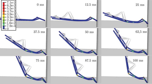
A race kart is a vehicle characterized by simplicity. The racing kart is depicted in Figure 2. The main components of a racing kart are the motor, the steering assembly, the four tyres, the rear axles, the seat and the kart frame, which has the function to carry all those parts. A race kart does not have any suspension or shock absorbing system; hence its dynamic behaviour is strongly influenced by the structural characteristics of the frame. Therefore, the kart frame, as shown in Figure 3, in combination with the point masses representing the driver, motor and bearings, is an ideal simple example to discuss the performance of various MOR methods in a crash simulation. The non-constant forces F_i and torques M_i, i ∈ {1, 2, 3,4,5} represent the interactions between the kart frame, the tyres and the rear shaft. Those interactions are important for the simulation of the whole vehicle. However, in this work we are only interested in the deformation behaviour of the kart frame and therefore tyres and rear shaft are not considered during the crash of the frame into the rigid pole (see Figure 3). Nevertheless, if we want to include the kart frame in a whole vehicle simulation, the interactions need to be considered in the MOR process as inputs respectively boundary conditions to the kart frame. A kart frame is mainly composed of steel pipes. For the modelling of the steel pipes, thin-walled shell elements are used because they are much more suitable than solid elements. As explained in [33], the geometric data of the kart frame was obtained by measurements. For the analysis of the noise, vibration and harshness (NVH) behaviour as done in [33], the kart frame was meshed with an automated meshing algorithm from Ansys. For the NVH analysis, the automated mesh with some small elements was suitable. For explicit crash simulations, however, a regular rectangular mesh with a constant mesh size is preferable in order to restrict the time step size. The more regular rectangular mesh was created in a semi-automatic way in Hypermesh. The point masses are connected by bushing elements consisting of light, stiff beams. Kart frames as well as bicycle frames often consist of hardened and tempered 25CrMo4 steel. The steel is characterized by a high toughness despite its high strength and hardness. The elastic-plastic characteristic of the steel frame is given as LS-DYNA Material 24: *MAT_PIECEWISE_LINEAR_PLASTICY with a stress-strain curve for the plastic deformation obtained from [34] that is defined at 10 points. For the bushing elements, light and stiff linear elastic beams are defined, which ensure an almost rigid coupling between driver/engine and frame. To research the behaviour of linearly reduced parts in a crash simulation, the racing kart is crashed frontally into a rigid pole. The dimension of the pole is in accordance with the dimension of the rigid pole used in the European New Car Assessment Program (EuroNCAP) [35] for side crashes. The pole and floor are modelled by rigid walls and it is ensured that no intersection occurs between the kart frame and the rigid walls with a standard LS-DYNA *CONTACT_AUTOMATIC. An explicit automatic time-stepping integrator without mass scaling is used to simulate the nonlinear deformation behaviour of the kart from 0 to 100 ms. In Figure 4, the kinematic behaviour and deformation are depicted for a central crash with an initial velocity v₀ of 32 km/h. The frontal part of the kart frame hits the rigid pole and slides towards the bottom. The frontal pipe is deformed and the kart frame buckles in the middle due to the high inertia of the driver and engine.

Figure 4. Kinematics of the original (unreduced) central crash with 32 km/h. The legend indicates the plastic strain.

3.1. Offline simulations to identify areas of small and large deformation

In order to determine which parts of the model exhibit large deformations and which can be modelled linearly, it is necessary to run multiple simulations with varying parameters, e.g. impact velocity or impact position in an offline simulation step, as depicted in Figure 5. The kart crashes with three different initial velocities v₀ = {15 km/h, 25 km/h, 32 km/h} and at three different locations – right, central and left, into the rigid pole. For the right and the left offset crash, the pole is moved by 212.5 mm from its central position. The inner border of the pole is therefore located at 40% width of the frame during the offset crash. The position of the pole is similar to the 40% ‘Offset Deformable Barrier’ frontal crash test from the Euro NCAP consortium where the offset is used to initiate a rotation of the car in frontal impact scenario.

Figure 5. Initial condition of the offline simulations to determine areas with ‘linear’ and ‘nonlinear’ behaviour. The crash position of the pole is labelled with left, central and right.

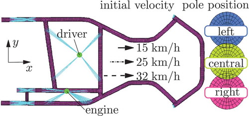
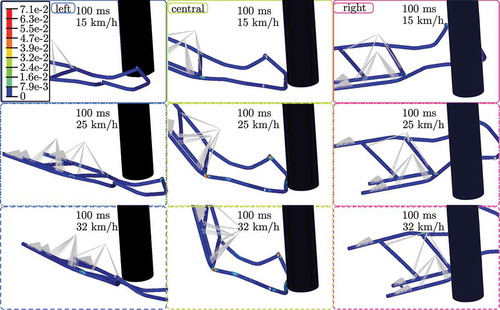
Accelerations of the driver, which are Channel Frequency Class (CFC)-1000 filtered, are visualized in Figure 7. A CFC Filter is a fourth pole backward–forward low-pass filter with a corner frequency of 1650 Hz used to cancel out high frequency oscillations. The driver experiences an acceleration of 18 g when he hits the right offset pole with maximum velocity. In general, the accelerations are larger for the right offset and central crashes in comparison to the left offset crashes due to the non-symmetric mass distribution towards the right side. In Figure 8, the final positions at t = 100 ms and plastic strains of the racing kart are depicted when the simulations are started with different initial values. The effective plastic strain in LS-DYNA is a monotonically increasing scalar value defined by the integral over the plastic component of the deformation rate tensor. The rows of the figure represent the initial velocities v₀ = {15 km/h, 25 km/h, 32 km/h} and the columns represent the three different locations of impact (left, central, right) into the pole. In the left and the right offset crashes, the kart hits the pole, is deflected and slides sideways past the pole. Therefore, the plastic strains seen in offset crashes are smaller than those of the central crash. As expected for the central crash with the largest initial velocity, the plastic strain is maximum in the middle of the kart where the frame folds. After 100 ms, there is 67% plastic strain for some elements in the crumple zone in the middle of the kart. Similar to passenger cars in frontal crashes, the deformation is rather small in the rear part of the kart. In Figure 8, the colour scale is deliberately chosen to visualize low values, with plastic strain values above 7% depicted in red. No plastic deformation occurs in the rear part of the kart. As a consequence, these parts are approximated as linearly reduced elastic bodies. The kart frame is cut into two parts, depicted in Figure 6. The steel pipes are cut into five positions and all nodes on the rim are defined as interface nodes at each cut circle. In total, the model contains 70 interface nodes, shown in cyan.

Figure 6. Frame cut into a frontal nonlinear described part and a rear linear described part.

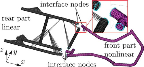
Figure 7. Acceleration of the driver for v₀ = 32 km/h, where left, central and right refer to the position of the pole.

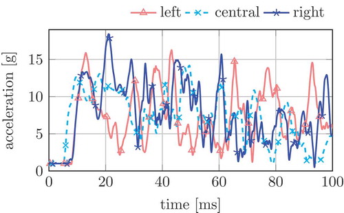
Figure 8. Final positions and effective plastic strains of the racing kart. The offline simulations are performed to determine linear and nonlinear behaviour of the kart. The rows of the figure represent the initial velocities v₀ and the columns represent the three different locations of the pole.

In Table 1, the number of elements, nodes and DOF are given for the frontal part and the rear part.

Table 1. Number of elements and nodes for the split model.

	Kart parts
	Front	Rear
# elements	4304	5727
# nodes	4244	5174
# DOF	25,464	31,044

4. Results

Once the full nonlinear kart model is split into frontal and rear parts, both parts of the model are linearized and imported into MatMorembs [19]. The models are then reduced with several approaches in order to find optimally reduced substructures in terms of approximation quality of the assembled linear system. Afterwards, the linearly reduced model of the rear part and the still nonlinearly described frontal part are assembled and simulated in LS-DYNA.

4.1. Optimal reduction of linear substructures

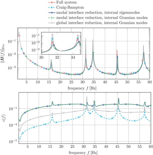
A frequency domain analysis is performed for the kart model, consisting of separately reduced frontal and rear parts. The transfer matrix is calculated with the force excitation located at the interfaces between the substructures and observed deformations at the driver’s seat. Linearized rigid body motion is allowed, similar to the crash test scenario. We want to generate a reduced rear substructure that can be used in the nonlinear crash simulation. The linearized analysis is used to perform a pre-selection of suitable methods. A good approximation of the transfer matrix of the assembled system qualifies the tested methods for the nonlinear simulation. The quality is measured by the transfer function of the error system and results in the relative error measure using Frobenius norms

(14) $ϵ(f)=\frac{\parallel H(f)-\bar{H}(f){\parallel }_{\mathrm{F}\mathrm{r}\mathrm{o}}}{\parallel H(f){\parallel }_{\mathrm{F}\mathrm{r}\mathrm{o}}}$(14)

All these pre-selective tests can be performed with a linear model with comparatively low computational effort.

While a straightforward modal or balanced truncation on substructure level fails for analyses of this type [17], it is shown in Figure 9 that accurate results can be obtained with a variety of methods. Multiple interfaces with a total of 420 interface DOFs are contained in the model. Therefore, using brute-force constraint modes produces a model with 420 DOFs, including six rigid body DOFs and the Craig–Bampton method thus results in a large reduced system. This problem will become worse for industrially used models, as they are usually meshed even more densely and, therefore, contain more DOFs at the interface. Reducing the interface ansatz functions leads to much smaller models. From Figure 6, we can identify five surfaces of interface nodes, each resulting in a separate interface. However, if only six modes per interface are considered, approximation quality does not improve with alternative reduction schemes applied only to the internal dynamics. If the interface deformations are computed with the help of a balanced truncation scheme applied on the assembly level, a better approximation is achieved. Obviously, the selected type of interface reduction is the dominant factor for the quality of the partially reduced kart model. The presented methods yield reduced models that exhibit a dynamic behaviour similar to the full linearized model and, therefore, are also considered for the nonlinear crash simulation in LS-DYNA.

Figure 9. Norm of the transfer matrix of full and reduced systems and the corresponding error measures.

4.2. Influence of reduction methods on the nonlinear crash simulation

The model consisting of a linearly reduced part and a nonlinear part is simulated with LS-DYNA in the online step. Therefore, the mass orthogonal ansatz functions are exported from MatMorembs into a .d3eigv binary file from which LS-DYNA calculates the equation of motion of the reduced elastic body. The coupling between the reduced and full nonlinear frontal part is achieved by merging the interface nodes on the rims.

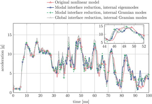
To evaluate the performance of the applied approach, the accelerations of the driver calculated with various reduction and parameter settings are compared with the accelerations measured when the original, unreduced nonlinear model is simulated. In Figure 10, the results are depicted for the central crash with 32 km/h. For the first 30 ms, the results of the original model and the reduced models fit very well, with an error smaller than 2 g. After 30 ms, the kinematics between the reduced and unreduced models changes slightly and therefore, the acceleration of the driver changes slightly too. Mainly, the timing of the peaks varies. In general, the main acceleration peaks occur later for the original model. However, the maximum error between the acceleration of the unreduced model y_full and the various reduced y_red is still less than 6 g. The results of the different reduction methods are very similar. For this reduction size there is not much difference between the usage of internal Gramian modes and the usage of internal normal modes. Both models have 6 rigid body DOFs plus 51 elastic DOFs. The size of the reduced system was selected based on the decay rate of the Hankel singular values of the internal Gramian modes. For comparison reasons, all reduced models are the same size. The use of global interface reduction does not – in contrast to the linear substructure tests – improve the approximation quality.

Figure 10. Acceleration of the driver for v₀ = 32 km/h in a central crash. The results are calculated with different simulation models where the reduced models are calculated with different reduction approaches.

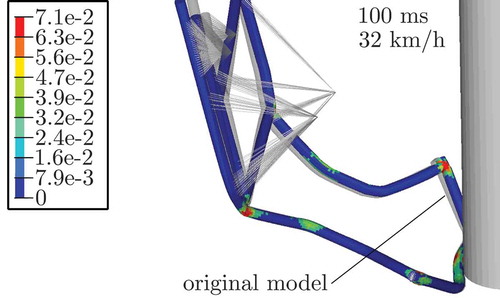
In addition, the plastic strain of the reduced (CMS Gram with modal interface reduction) nonlinear model is calculated and depicted in Figure 11. The maximum plastic strain is 61% which is very similar to the original strain, and the maximum strain occurs at the same positions as for the original model, see Figure 4 or Figure 8. Furthermore, the final state of the original model is also depicted in Figure 11, and the small difference between the full and the reduced models can be seen.

Figure 11. Plastic strain of the deformed reduced model (CMS-Gram with modal interface reduction) plus the kinematics of the unreduced model for the central crash.

The runtime of the different models in LS-DYNA is summarized in Table 2. All results were obtained using a standard computer (Intel i7-3770 [email protected] GHz, 32 GB RAM) using only one core. The online calculation times for the reduced models except Craig–Bampton are very similar and, therefore, not further compared among themselves. Therefore, only the simulation times for the reduced model with modal interface reduction and the usage of internal Gramian modes are listed in Table 2. After the simulation results justified the usage of linear reduced models in combination with nonlinear models, the runtime improvement of the reduced model in comparison to the original model is rather disappointing. The advantage of fewer and, therefore faster element processing, 0.97.10³s vs. 2.21.10³s, is devoured by the time needed to calculate the reduced elastic body (1.26.10³s). From a theoretical point of view and from the experience gained in other projects, the simulation time of the reduced elastic body should be much faster than the current implementation in LS-DYNA. Reasons for the unsatisfying simulation time could be the ratio between the to-be reduced DOF N = 31,044 to the number of interface DOFs $414$ or the implementation for the reduced elastic body in LS-DYNA. It is rather surprising that the few matrix multiplications of 51 × 51 matrices take as long as the element processing for 5727 elements. Based on our experience, the simulation of a reduced elastic body of dimension 51 should be much faster. If the size of the reduced model is further decreased, e.g. to ten, we can achieve slightly faster computations but the results of the reduced model are no longer sufficiently in accordance with the original model. The application of the brute-force Craig–Bampton method without an interface reduction produces a large reduced model with a very high maximum eigen frequency. Therefore, the maximum stable time step is rather small (3.9 ns). If we use four cores in parallel to simulate the reduced system, more than 11.3 days of processing time are needed for 38 million problem cycles. The unreduced model on the other hand has a maximum stable time step of 162.5 ns and only 0.6 million problems cycles are calculated in 65 min using only one core. Therefore, standard brute-force Craig–Bampton methods are not a convenient choice for industrial crash applications in the presented setup due to the high interface number.

Table 2. Calculation times in LS-DYNA.

	Original		CB^[^1^]
	CMSG-IR^[^2^]
Elapsed time [10^3s]	3.9	3.75	3935
Element proc.^[^3^] [10^3s]	2.21	0.97	94.9
El. body proc.^[^4^] [10^3s]		1.26	3582
Problem cycles [10^6]	0.63	0.63	38.18
Mean time step [ns]	150	150	2

^[1] Standard Craig–Bampton;

^[2] CMS Gram with modal interface reduction;

^[3] Element processing;

^[4] Elastic body processing.

5. Conclusions

This work presents an approach to save simulation time in explicit crash simulations of vehicles. In order to determine which parts of the kart frame exhibit rather large deformations and which can be modelled linearly, it was necessary to run multiple simulations with varying parameters, e.g. impact velocity and pole position in an offline step. Afterwards, the frame was cut into two parts and the rear part was linearly approximated with the MOR programme MatMorembs. In a first step, the frontal and the rear part were reduced with several approaches in order to find optimally reduced substructures. Based on the results from a linear substructure analysis, the model consisting of a linearly reduced part and a nonlinear part was simulated with LS-DYNA in the online step. The correct coupling between reduced and original models and the setup of the reduced elastic body in LS-DYNA were the most challenging part of this research. No meaningful results were obtained using the standard approach from LS-DYNA to simulate reduced elastic bodies. This is due to the fact that LS-DYNA leaves rigid body modes in the elastic ansatz functions which leads to unpredictable and incorrect wrong simulation results. However, once the elastic ansatz functions are calculated, mass orthogonalized in MatMorembs and exported to a .d3eigv file, the results of the reduced model are very similar to the results of the full original nonlinear model. While a clear advantage of global-reduction approaches in the linear optimal substructure calculations can be observed, we do not see this advantage for the nonlinear time simulations. In addition, the simulation speed up is still of mediocre quality. We hope to improve the simulation speed up in the future. Due to the high number of interface nodes, correct handling of the interfaces between the linearly approximated and nonlinear parts [18] is essential for good results. The brute-force Craig–Bampton method is not suitable for the usage in industrial crash models due to the high number of interfaces which leads to high eigen frequencies of the reduced body and, therefore, a small maximum stable time step, which slows down the calculation time exorbitantly.

So far, only the feasibility of the method was researched with the kart frame. In future steps, the same approach should be tested for a full-scale passenger car to decide if the combination of linear reduced parts and nonlinear original parts in crash simulations is a promising way to save simulation time or if nonlinear reduction techniques are necessary to speed up crash simulations.

Acknowledgements

The authors would like to thank the German Research Foundation (DFG) for financial support of the project within the Cluster of Excellence in Simulation Technology (EXC 310/1) at the University of Stuttgart. This research was partly assisted by Bünyamin Tezcan, who helped with the FE modelling, the FE converter and did some of the FE simulations during his bachelor thesis. In addition, the authors would like to thank the reviewers for their comments that helped improving the manuscript.

Disclosure statement

No potential conflict of interest was reported by the authors.

Additional information

Funding

This work was supported by the Deutsche Forschungsgemeinschaft [EXC 310/1].

References

- R. Isermann, Mechatronic Systems: Fundamentals, Springer, London, 2005.
- P. Eberhard and W. Schiehlen, Computational dynamics of multibody systems: History, formalisms, and applications, Trans. ASME J. Comput. Nonlinear Dyn. 1 (2006), pp. 3–12.
- P. Goupil and A. Marcos, Advanced diagnosis for sustainable flight guidance and control: The European ADDSAFE Project. Technical Paper 2011–01–2804, SAE International, 2011.
- C. Tobias, J. Fehr, and P. Eberhard: Durability-based structural optimization with reduced elastic multibody systems. In Proceedings of the 2nd International Conference on Engineering Optimization, Paper-ID 1119, Lisbon, Portugal, September 6–9, 2010.
- A. Tkachuk and M. Bischoff, Variational methods for selective mass scaling, Computational Mechanics 52 (3) (2013), pp. 563–570. doi:10.1007/s00466-013-0832-0
- V. Faucher and A. Combescure, Local modal reduction in explicit dynamics with domain decomposition. Part 1: Extension to subdomains undergoing finite rigid rotations, Int. J. Numer. Methods Eng. 60(15) (2004), pp. 2531–2560.
- T. Borrvall, D. Bhalsod, J.O. Hallquist, and B. Wainscott: Current status of subcycling and multiscale simulations in LS–DYNA. In 13th International LS-DYNA User Conference, Detroit, USA, 2014.
- A. Antoulas, Approximation of Large-Scale Dynamical Systems, SIAM, Philadelphia, 2005.
- P. Benner, V. Mehrmann, and D. Sorensen (Eds.), Dimension Reduction of Large-Scale Systems, Vol. 45 of Lecture Notes in Computational Science and Engineering, Springer, Berlin, 2005.
- W. Schilders, H. Van Der Vorst, and J. Rommes, Model Order Reduction: Theory, Research Aspects and Applications, Vol. 13 of Mathematics in Industry, Springer, Berlin, 2008.
- A. Quarteroni and G. Rozza, Reduced Order Methods for Modeling and Computational Reduction, Vol. 9 of MS&A - Modeling, Simulation and Applications, Springer International Publishing, Switzerland, 2014.
- J. Fehr and D. Grunert, Model reduction and clustering techniques for crash simulations, PAMM 15 (1) (2015), pp. 125–126. doi:10.1002/pamm.201510053
- B. Bohn, J. Garcke, R. Iza-Teran, A. Paprotny, B. Peherstorfer, U. Schepsmeier, and C.-A. Thole, Analysis of car crash simulation data with nonlinear machine learning methods, Procedia Comput. Sci. 18 (2013), pp. 621–630. doi:10.1016/j.procs.2013.05.226
- L. Mei and C. Thole, Data analysis for parallel car-crash simulation results and model optimization, Simul. Modell. Pract. Theory 16 (3) (2008), pp. 329–337. doi:10.1016/j.simpat.2007.11.018
- B. Miled, D. Ryckelynck, and S. Cantournet, A priori hyper-reduction method for coupled viscoelastic viscoplastic composites, Comput. Struct. 119 (1) (2013), pp. 95–103. doi:10.1016/j.compstruc.2012.11.017
- C. Farhat, P. Avery, T. Chapman, and J. Cortial, Dimensional reduction of nonlinear finite element dynamic models with finite rotations and energy-based mesh sampling and weighting for computational efficiency, Int. J. Numer. Methods Eng. 98 (9) (2014), pp. 625–662. doi:10.1002/nme.4668
- P. Holzwarth and P. Eberhard, SVD-based improvements for component mode synthesis in elastic multibody systems, Eur. J. Mecha. A/Solids 49 (2015), pp. 408–418. doi:10.1016/j.euromechsol.2014.08.009
- P. Holzwarth and P. Eberhard: Interface reduction for CMS methods and alternative model order reduction. In Proceedings of the MATHMOD 2015 – 8th Vienna International Conference on Mathematical Modelling, Vienna, Austria, 2015. 10.1016/j.ifacol.2015.05.005
- P. Holzwarth, M. Baumann, T. Volzer, I. Iroz, P. Bestle, and J. Fehr, Software Morembs, University of Stuttgart, Institute of Engineering and Computational Mechanics, Stuttgart, Germany, 2015.
- B.N. Maker and D.J. Benson: Modal methods for transient dynamic analysis in LS-dyna. In Proceedings of the Seventh International LS-Dyna Users Conference, Detroit, USA, 2002.
- T. Belytschko, W.K. Liu, and B. Moran, Nonlinear Finite Elements for Continua and Structures, John Wiley & Sons, Chichester, 2000.
- P. Wriggers, Nonlinear Finite Element Methods, Springer, Berlin, 2010.
- R. Craig: Coupling of substructures for dynamic analyses: an overview. In Proceedings of the AIAA Dynamics Specialists Conference, Paper-ID 2000-1573, Atlanta, April 5, 2000.
- J. Fehr, Automated and Error-Controlled Model Reduction in Elastic Multibody Systems. Dissertation, Schriften Aus Dem Institut Für Technische Und Numerische Mechanik Der Universität Stuttgart, Vol. 21, Shaker Verlag, Aachen, 2011.
- P. Holzwarth and P. Eberhard: Interpolation and truncation model reduction techniques in coupled elastic multibody systems. In Proceedings of the ECCOMAS Thematic Conference on Multibody Dynamics, Barcelona, Spain, 2015.
- B. Salimbahrami and B. Lohmann, Second order krylov subspace for the reduction of second order systems, in Methods and Applications in Automation, 25th - 26th Colloquium of Automation, Salzhausen, Germany, No. 1.1 in Publication Series of the Institute of Automation, University of Bremen, A. Gräser and B. Lohmann, eds., Shaker Verlag, Aachen, 2005, pp. 1–11.
- J. Fehr, M. Fischer, B. Haasdonk, and P. Eberhard, Greedy-based approximation of frequency-weighted gramian matrices for model reduction in multibody dynamics, Zeitschrift für angewandte Mathematik und Mechanik 93 (8) (2012), pp. 501–519. doi:10.1002/zamm.201200014
- T. Wolf, H. Panzer, and B. Lohmann, Model order reduction by approximate balanced truncation: a unifying framework, at-Automatisierungstechnik 61 (8) (2013), pp. 545–556. doi:10.1524/auto.2013.1007
- M. Lehner and P. Eberhard, A two-step approach for model reduction in flexible multibody dynamics, Multibody Syst. Dyn. 17 (2–3) (2007), pp. 157–176. doi:10.1007/s11044-007-9039-5
- M. Burkhardt, P. Holzwarth, and R. Seifried, Inversion-based trajectory tracking control for a parallel kinematic manipulator with flexible links, in Proceedings of the 11th International Conference on Vibration Problems, Z. Dimitrovová, J. De Almeida, and R. Gonçalves, eds., Lisbon, September 9–12, 2013.
- J.L. Eftang and A.T. Patera, A port-reduced static condensation reduced basis element method for large component-synthesized structures: approximation and a posteriori error estimation, Adv. Modell. Simul. Eng. Sci. 1 (1) (2014), pp. 3. doi:10.1186/2213-7467-1-3
- S. Donders, B. Pluymers, P. Ragnarsson, R. Hadjit, and W. Desmet, The wave-based substructuring approach for the efficient description of interface dynamics in substructuring, J. Sound. Vib. 329 (8) (2010), pp. 1062–1080. doi:10.1016/j.jsv.2009.10.022
- T. Shiiba, J. Fehr, and P. Eberhard, Flexible multibody simulation of automotive systems with non-modal model reduction techniques, Vehicle Syst. Dyn. 50 (12) (2012), pp. 1905–1922. doi:10.1080/00423114.2012.700403
- Total Materia Werkstoffdatenbank. www.totalmateria.com, accessed June 21, 2015.
- Euro NCAP: European New Car Assessment Programme (Euro NCAP): assessment protocol – adult occupant protection, Version 7.0.2. Tech. rep., Euro NCAP, 2 Place du Luxembourg, 1050 Brussels, Belgium, 2015.