Modelling game sports as complex systems – application of recurrence analysis to golf and soccer

ABSTRACT

Analyses of game sports or of performances shown in them require appropriate models. Many game sports can be modelled as complex, dynamic systems. This study investigated how recurrence plots (RPs) – a method to analyse complex systems – and the analyses of RPs can be applied to the game sports golf and soccer. A golfer is treated as a complex system with many unknown components. The scalar variable Shots Saved can describe his/her behaviour. Phase space reconstruction is needed to unfold hidden facets of a golfer’s behaviour. Results indicate that golfers’ performances do not approach a stable state, but seem rather unpredictable. A soccer match can also be treated as a complex system. Some components – the players – and their respective behaviour represented by movement trajectories are known and can be used to describe the system’s behaviour. We propose that no embedding is needed for the RP construction in this case. Results indicate that the more goal shots there are in a game, the more unstructured it is. Furthermore, if several golfers or soccer matches are investigated, we recommend using the same RP parameters to achieve comparable results.

KEYWORDS:

• Recurrence plot
• game sports
• performance analysis

Introduction

Analysing performances shown during sports competitions has become a rapidly growing field in the more recent past. For that, appropriate methods are required to analyse performances in different sports. The performance structure differs from sport to sport. For example, performance in endurance sports is mostly based on performance prerequisites such as athletic ability and technical and tactical skill. An athlete’s 100 m sprint performance might be predicted within narrow margins knowing the actual level of reaction time, acceleration, maximum speed and speed endurance from prior, separate testing. In contrast, the performance in many game sports emerges from a dynamic process which is characterized to a great extent by the interaction between the athletes, although their athletic abilities and technical and tactical skills also influence performance.

In the past, different approaches have been used to assess game sport behaviour. One approach focuses on investigating game-specific actions using performance indicators such as ratios of completed passes, or other descriptive methods such as the analysis of pass sequences [1]. Subsequently, these parameters are studied with respect to their relation to match-winning actions such as scoring goals, using inferential statistics, e.g. [2–4]. However, such performance indicators only describe isolated aspects of the respective game sport [5,6].

Another approach is to model athletes and game sports as complex, dynamic systems. Human behaviour is based on the interaction of many components providing a large number of degrees of freedom. In a simple case, for example, a finger of a person has a limited number of degrees of freedom. Although one might be able to count the degrees of freedom involved, the task plays an important role which the person performs the finger belongs to. For example, the person could play a PC game by clicking the mouse with the finger in question or he/she could play a sophisticated piano concerto. However, it is obvious ‘that the amount of information that is transmitted by […] [the] biomechanical degree[s] of freedom in the complexity of motion is vastly richer than any counting of mechanical degrees of freedom would suggest’ [7, p. 41]. Observable human behaviour emerges from the synergy of a lot of components, such as mechanical or neuronal components [7]. A specific type of behaviour such as a golf shot can reach a stable pattern through learning (if exercised often enough) and can be reproduced within a small range of variability. The relationships between the interacting components are non-linear. A small change in the hip angle might influence the outcome of a golf shot marginally, whereas a slightly rotated arm usually has a large effect on the angle of the club head, and thus the golf ball curves to the right. This complex systems approach has been applied at many levels of the analysis of human movement and performance, see e.g. [7–9], and is appropriate for modelling individual athletes and their performance in game sports [7].

Game sports such as soccer can also be modelled as complex, dynamic systems [10,11]. In a soccer match, there are usually 22 players. The players are coupled with each other in different ways. There are intra-couplings as well as inter-couplings [11]. Intra-couplings describe the couplings within a soccer team. For example, each player of a team is initially coupled with his/her immediate neighbours on the pitch. However, there are many more intra-couplings amongst the players of a team and they keep changing depending on the game’s context. Inter-couplings describe relations between players of different teams such as the coupling between a defender and a striker or between two midfielders of different teams. Due to alternating ball possession, a soccer match shows ‘a to-and-fro behaviour more reminiscent of a tidal ebb-and-flow’ [11, p.773]. Depending on this behaviour, intra- as well as inter-couplings are generated or broken regarding the current game context, which is determined by which team is in possession of the ball and the corresponding positioning of all players on the pitch. For instance, team A gains ball possession and starts a counterattack. Then the team B players try to achieve a well-organized defensive line-up. During this, different players from team B (e.g. a striker and a defender) can be direct neighbours and are coupled differently than during a well-organized defensive team line-up.

During ball possession, a team tries to keep possession and score a goal, and the other team simultaneously tries to (re)gain ball possession and prevent the team in possession from scoring. Thus, once the defence of team B and the offence of team A have achieved well-organized line-ups, the teams neutralize each other and stable player patterns occur. The couplings are non-linear, since a player’s error can have either nearly no effect or a very large effect if he/she opens up space and, as a consequence, the team in possession of the ball gets a scoring opportunity. Furthermore, the state of a match at time t_i+1 emerges from the players’ behaviour at time t_i. Additionally, the complex dynamic system soccer match is a nested system since some of its components – the players – are complex dynamic systems themselves.

Physical sciences provide a variety of concepts and tools which are suitable for understanding and analysing the behaviour of complex systems. For example, the dynamical systems theory, widely used in game sport analyses, provides theoretical concepts such as self-organization [12], affordances [13] or constraints [14] which are used to analyse a system’s observable behaviour qualitatively [5]. On the other hand, there is a variety of methods to quantify, and subsequently statistically analyse, a complex system’s behaviour. Amongst others, such methods are the relative phase, measures of complexity and synchrony – such as the approximate entropy – or recurrence analysis. Relative phase, e.g. [15–20], and complexity measures, e.g. [21,22], have been applied to game sports frequently. For example, relative phase analyses have identified soccer [17,18] and basketball [19,20] as in-phase games outlining a very close inter-coupling between teams regarding longitudinal (goal to goal or basket to basket) movement direction. Furthermore, it was possible to identify some phases as scoring opportunities, when the teams were less strongly coupled. However, for technical reasons relative phase only allows the coupling to be analysed taking one movement direction into consideration. The application of recurrence plots (RPs), a tool for visualizing recurring patterns of complex, dynamical system behaviour, and recurrence quantification analyses (RQAs) [23] – which allow the structures in RPs to be quantified – to game sports is relatively new. So far, the authors of this study are only aware of one study which has applied RQA to game sports, its application to tennis. The players’ relative positioning during baseline rallies was investigated, and the results showed that RQA helped to identify rally breaks leading to points [24].

A similar method to RP and RQA is the T-patterns approach. It allows the analysis of time series data sets regarding recurring structures [25]. This method has been used to detect and to describe recurring sequences of behavioural events. In contrast to the RP approach, where the underlying data are interval-scaled, the T-patterns are based on categorical event data which describe the beginning and the end of certain behaviour performed by an agent. The T-patterns approach has already been applied to investigate some game sports, including soccer [26]. The event categories in this soccer research were pass, tackle, header or run, and the field of play was separated into discrete zones. A correlation showed a close relation (r = .81) between the number of patterns found for a team and an assessment of the team’s performance by experts. The more structured the manner in which a team played, the better it was.

Considering the findings of research [26], and due to the similarity of the methods, RP and RQA seem to be promising approaches for shedding light on game sport behaviour. The RP analyses are based on the positional information of players in this research and thus focus on the dynamic of the game rather than on specific events.

In golf, the developments in the more recent past have led to measurements which allow the performance of a shot to be quantified in terms of its outcome [27,28]. The existence of such measurements allows more detailed analyses regarding the performance structure, such as ‘Are there phases when golfers’ style of play is more stable or unstable?’ or ‘How predictable are performances?’. Furthermore, amongst experts, fans and also athletes there is the belief that ‘success breeds success and failure breeds failure’ [29, p. 525]. This phenomenon, called streakiness or hot-hand, has been investigated already, but only based on round or hole scores due to the data available. However, only weak support was reported for this belief [30–32]. Such open golf questions could be approached on a shot-by-shot level using RP and RQA.

This paper illustrates the application of the RP method to golf and soccer. In both sports, progress in information technologies has led to the collection of a huge amount of data during competitions. During golf competitions, data on each shot of each golfer is collected, at least during tournaments of the American professional golf tour, the US PGA TOUR. During soccer matches, positional data is collected for every player on the field of play. The existence of such data allows for the progress of the complex, dynamic system golfer as well as the progress of the complex, dynamic system soccer match to be described during a competition. The emphasis of this paper is on the technical aspects of the method’s application to both sports – the construction of RPs – rather than the application of the method from a sport scientific viewpoint, for instance a detailed analysis of performances using RP and RQA. However, for both sports a sport scientific application will be illustrated shortly.

The paper is outlined as follows: first, there is a short overview on RP and RQA. Then, the technical details of their application to golf are presented, followed by a short sport scientific application; and finally, the technical details of their application to soccer are presented followed by a short sport scientific application.

Recurrence plots

The RP concept

An RP is a tool for visualizing similarities within time series of complex, dynamic systems. Recurring patterns of a system can be identified in a symmetric N×N graphic, where N is the length of the time series. Generally, RPs can be divided into three categories according to the pattern of the recurrence points regarding the whole plot (large-scale texture) [33]: homogeneous plots (stationary process), periodical plots (oscillating process) and drift plots (transmuting process). Furthermore, the local patterns of an RP (small-scale textures) provide detailed information on the complex system’s behaviour during a certain time period. The most important small-scale textures are [23]:

• Isolated recurrence points (recurrence points without neighbours) indicate rare states or high fluctuation.

• Diagonal lines describe that the investigated system’s trajectories run parallel and close to each other for a certain time.

• Vertical (or horizontal) lines illustrate that the system remains in a state or very slowly moves in the neighbourhood of a state for a certain time.

• Clusters of recurrence points mean that vertical and horizontal lines occur at the same time, forming blocks.

• White space or bands refer to states which are rare or only occur once.

Depending on the characteristics of the analysed complex system, the types and the amount of occurring small-scale textures usually vary. For example, deterministic processes cause longer diagonal lines in their RPs than chaotic processes, whose RPs are dominated by isolated recurrence points [23].

RP construction

The construction of RPs involves several steps which will be introduced in this subsection. The details of the RP construction applied to golf and to soccer will be discussed in the following sections.

The investigated complex system’s behaviour is often measured as scalar, discrete time series a₁,…,a_N, since not all relevant components of a system are known or can be measured. According to Takens [34], the original time series needs to be expanded to a higher dimensional phase space in order to unfold the real system’s dynamics. The so-called phase space reconstruction is often realized using a time delay method [23]. This method requires two parameters to be chosen properly, the embedding dimension m and the time delay tau, $m,tau\in \mathbb{N}$ [23,35,36]. These parameters are frequently determined using a false nearest neighbour algorithm for the embedding dimension and an autocorrelation or mutual information function for the time delay. False nearest neighbours are phase space points that are close to each other in dimensions smaller than the original dimension of the investigated system in which these points are not close to each other. The method used in this paper [37] considers the amount of false nearest neighbours as a function of the embedding dimension. An appropriate embedding dimension is found when the number of false nearest neighbours approaches zero [37]. The autocorrelation function assesses dependences between the measurements at different times. An appropriate tau is found when the function approaches zero [38]. Mutual information involves a function expressing ‘the average of the information about a value after a delay tau, which can be yielded from the knowledge of the current value’ [38, p. 6]. According to the research [38], an appropriate tau is where the mutual information function has its smallest local minimum.

Based on m and tau, the measured time series is embedded into a higher dimensional phase space where the progress of the system is represented by a series of vectors b_i = (a_i, a_i+1*tau,…, a_{i+(m−1)*tau})^T, i = 1,…,N – (m – 1)*tau. However, there are discussions on whether an embedding is necessary for the RP construction [35,39]. In such cases the RP construction is conducted with tau = 1 and m = 1.

Independent of the decision to embed or not to embed, the similarity of states needs to be determined. It is usually assessed using a distance measure, such as the absolute value norm (finding the lowest number of neighbours), the Euclidean norm (finding an intermediate number of neighbours) or the maximum norm (finding the highest number of neighbours). According to [23], all these norms are appropriate and can be chosen with respect to the computational speed; for instance, the maximum norm is the fastest. States are treated as similar and are also called recurring states, if the distance between them is smaller than a predefined threshold ε [23]. Determining an appropriate ε is crucial since it is important that not every state is similar to all others and, on the other hand, too small a value results in a nearly empty RP. In these cases the RP would not provide meaningful information on the recurring structures anymore. There are several approaches to choosing ε which are accepted for delivering the appropriate thresholds, see [23] for an overview, e.g.:

• A frequently used approach to finding a proper ε is to make the threshold a few per cent of the maximum diameter of the phase space trajectory of the investigated system [40], but not greater than 10% [41].

• Marwan [42] states that it is important to achieve a high number of long diagonals while the variability of the lengths stays small to get as much information as possible from an RP. Therefore, the value of ε should be selected as the one where the ratio (number of recurrence points forming diagonal lines)/(variability of the length of the diagonal lines) reaches its maximum. The measurement of a complex system’s process is composed by the real values and noise. If the amount of noise is known, ε should be larger than five times the standard deviation of the observational noise.

Mathematically, an RP is represented by a matrix with binary entries

(1) $R{P}_{i,j}\left(\epsilon \right)=\Theta \left(\epsilon -\left|\left|b_i-b_j\right|\right|\right),i,j=1,,\dots ,N-m*tau,$(1)

where Θ is the Heaviside function and ||.|| is a norm, the chosen distance measure for assessing similarity between two states. The entries of RP are plotted colour coded, black usually indicates that two states are similar and white the opposite.

Recurrence quantification analysis

A method called RQA was developed to quantify structures in RPs [23,43]. Amongst other things, an RQA involves analyses of diagonal lines, vertical lines and the recurrence point density. The respective RQA parameters used in this paper are the rate of recurrence points in a plot (RR), the proportion of recurrence points forming diagonal (DET) and vertical lines (LAM), the average length of the diagonal (L) and the vertical lines (TT) and the variability in the length of the diagonal lines (ENTR).

For the RQA parameters which are based on diagonal and vertical lines, a minimum line length needs to be determined prior to it. The main reason for selecting the minimum line length with caution is in order to restrict the influence of tangential motion which ‘also [includes] points into the neighbourhood which are simple consecutive points on the trajectory’ [23, p. 247]. Furthermore, if the minimum is set too large the detected amount of diagonal lines in the RQA decreases and, consequently, the reliability of DET and LAM declines. Typically, the minimum line length is set two [38].

Applications to golf and soccer

This section thoroughly addresses the RP applications to golf and to soccer. In particular, the choice of parameters for the RP construction is described in detail. For the RP and RQA computations, the RP MATLAB toolbox provided by the authors of [23] was used.

RPs in golf

First, Shots Saved, a golf-specific performance indicator which describes the quality of individual golf shots, needs to be introduced briefly [28]. Basically, in this application the investigated dynamical system is the golfer and the system’s behaviour is described by Shots Saved values [28]. Since a golfer usually plays several shots at each golf hole and on a professional level a round is comprised of 18 holes, a round generates a sequence of shots, each of which can be assessed using Shots Saved values. Such a Shots Saved sequence can be considered as a discrete time series describing the respective golfer’s behaviour on the golf course on a shot-by-shot basis. Therefore, the RP approach based on a sequence of Shots Saved values is technically appropriate for studying the characteristics of golfers’ performances during competitions in principle.

In golf, each hole should be played with a certain number of shots, called par. Depending on the distance from the tee to the hole, there are par three, par four and par five holes. Research based on hole-by-hole analyses reveals that golfers on the PGA TOUR play par on about 60% of the holes [44]. Further research reported that in 60% of cases a par is followed by another par, whereas better and worse holes follow a par 20% of the time [32]. Thus, there are often stable phases when players play a few pars in a row. From a performance analysis perspective, this motivated us to conduct a pilot study of the performance of PGA TOUR golfers on a stroke-by-stroke basis using RP aimed at the question of whether there are such stable phases at a shot-by-shot level too. The recurrence analysis application described below is based on data from a PGA TOUR tournament, THE PLAYERS Championship 2011. It involves data from those 74 players who played all four rounds of the tournament (after two rounds there is a cut which only allows the better ranked half of the players to continue playing).

The ISOPAR method

The ISOPAR method is an approach developed to assess the quality of golf shots [28]. It relies on concepts of the dynamical systems theory, in the sense that the golfer as a human being can be considered as a dynamic system and that his/her behaviour on the golf course is constrained by influences from different sources [28]. For instance, such influences include the weather (e.g. wind, sun or rain) or the hole type (e.g. distance to the hole, surrounding area such as trees, or hardness and speed of the green). The golfers’ play can be influenced directly or indirectly by such factors. The golfers are directly influenced, for example, by a tree which blocks the straight line between the ball’s location and the hole. A factor indirectly influencing the golfers’ play would be a water hazard from which the golfers aim away for strategic reasons. Although this is not the shortest way to the hole, it limits the possibility of hitting the ball into the water, for which a golfer is penalized by an extra shot. Moreover, the golfers themselves are a source by which their play is constrained. A golfer needs to perceive the external factors, process this information to make a decision for the next shot and finally perform the intended shot as well as possible.

The ISOPAR method is based on ball locations and the respective number of remaining shots until the ball is holed. The number of remaining shots from a location represents the difficulty of this because the more difficult the location was, the more shots were needed. The difficulty is the result of the synergy of the abovementioned influencing factors. The ISOPAR method provides an algorithm for calculating the difficulty of holing the ball from any location at a golf hole. The resulting difficulty values are a weighted average of the remaining number of shots and are called ISOPAR values. Since the influencing factors are different from hole to hole, the difficulty is calculated for each hole separately. Furthermore, since a golf tournament is usually played over 4 days (one round a day) and each hole is played once a day, the ISOPAR value calculation is performed for each hole in each round to account for changing factors such as the weather (assuming that the weather during one given day is more stable than across 4 days) or the pin location, which is different in each round at each hole.

Based on the ISOPAR values, this method allows the quality of each individual shot to be assessed through the performance indicator Shots Saved [28]. For each ball location, an ISOPAR value can be determined. Considering the ball location before and after a shot allows a golfer’s performance to be assessed as shot quality (SQ) = ISOPAR value_{before –} ISOPAR value_after [28]. The Shots Saved value for a shot is defined as SQ – SQ_ave, where SQ_ave describes the average SQ of all golfers playing at the respective hole [28]. Thus, a Shots Saved value describes how much better or worse a golfer’s shot was compared to an average performance at a hole. A Shots Saved value of a shot is the ‘measurable’ outcome of the behaviour of the dynamic system golfer at this shot.

As described above, the quality of a golfer’s shot sequence in a tournament can be described by his/her Shots Saved series x₁,…,x_N, where N describes the number of shots the golfer took during the tournament. This Shots Saved series was used as the time series describing the golfer’s behaviour on which the RP is based.

RP construction

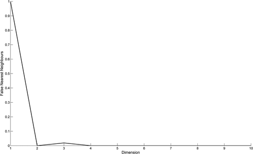
For the application to golf data, the use of phase space reconstruction was chosen to construct the RPs. The complex system golfer comprises a lot of unknown components and the interactions between them, and additionally the measurement describing the golfer’s performance is scalar. According to Takens [34], embedding phase space reconstruction is recommended. It was conducted using the time delay method. The respective parameters were determined using the mutual information algorithm and the false nearest neighbour algorithm both implemented in the used MATLAB toolbox [23]. The mutual information plots were visually inspected for all golfers in the data set (e.g. see Figure 1). The mutual information functions had their smallest local minima at time delay tau = 2. Subsequently, the embedding dimensions were determined based on the false nearest neighbours approach using tau = 2 (e.g. see Figure 2). The embedding dimension, where either no false nearest neighbours were left or the number of false nearest neighbours approached zero, was m = 2 for all golfers.

Figure 1. Mutual information function of one of the golfers at THE PLAYERS Championship 2011.

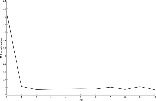
Figure 2. False nearest neighbour function of one of the golfers at THE PLAYERS Championship 2011 using tau = 2.

Using the phase space reconstruction based on m and tau, a recurrence threshold ε had to be determined. A frequently used approach was used to determine ε as a few per cent of the maximum diameter of the phase space trajectory of the investigated system, but not greater than 10%. Since for all golfers in the data set the reconstructed phase space had the same dimension, ε was decided to be the same for all golfers. Otherwise, the similarity of states would be assessed differently and the RPs would no longer be comparable. For instance, two states can be 0.05 Shots Saved apart from each other for one golfer and two states can be 0.2 Shots Saved apart from each other for another golfer, but in both cases the states are considered similar because of individual recurrence thresholds. Such unwanted effects affect the analysis of the RPs. Therefore, the following approach was used to determine ε, which is valid for all golfers:

• For each golfer the trajectory b_i, i = 1,…,N – (m – 1)*tau, in the reconstructed phase space was determined.

• Extreme outliers were removed from each trajectory to ensure that ε meets the maximum criterion of 10%. To identify extreme outliers, the approach suggested in [45] was used. There extreme outliers eo are defined as

$eo\{\begin{array}{l}<Q_{0.25}-3IQ\\ >Q_{0.75}+3IQ\end{array},$

where IQ is the interquartile distance and Q_i denotes the ith quartile of the distribution.

• For each golfer the recurrence threshold ε_i was determined as 10% of the diameter of the leftover trajectory.

• Finally, the recurrence threshold was computed as $\epsilon =\frac{1}{74}{\displaystyle \sum _{74}^{i=1}{\epsilon }_i}$.

The resulting ε was 0.14. In this application, the Euclidean norm was chosen as the distance measure for assessing the similarity of states in the reconstructed phase space as well as for the calculation of ε.

Using the parameters determined above, the resulting average RR based on all golfers’ RPs equals 6.9% (SD = 1.0%). Thus, the resulting RPs are sparse enough to allow an appropriate RQA according to Webber and Zbilut [46]. Therefore, the parameters for the RP construction were chosen sufficiently.

Sport scientific application

Figure 3 shows the RP of a golfer, K. J. Choi who won the tournament the data was taken from. The RP is characterized by many isolated recurrence points, a few clusters and short vertical lines as well as a few short diagonal lines. Therefore, Choi’s play can be interpreted as very fluctuating, but alternating with some short stable phases (vertical lines) from a sport scientific viewpoint using the suggestions of [23]. More-or-less white bands or sparsely populated bands can be identified in the RP as well, e.g. before shot 150. Those bands indicate that the quality of performance changed abruptly [23]; in other words, Choi played a few consecutive shots which he rarely played in this tournament, e.g. alternating extremely good and extremely bad shots. However, the RP itself does not provide information on how well or how bad Choi played at any given time.

Figure 3. Recurrence plot of K. J. Choi’s performance at THE PLAYERS Championship 2011 (m = 2, tau = 2, ε = 0.14); black dots represent recurring states.

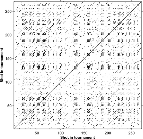
The absence of longer diagonal lines parallel to the line of identity raises the suspicion that Choi’s behaviour was not deterministic, but rather chaotic. The RQA analysis of Choi’s plot supports this assumption since DET = 16.2% and L = 2.4 (for DET the minimum line length was set two). Such small values indicate that the investigated system, and hence this golfer, behaved rather unpredictably/chaotically [45]. Choi’s LAM = 22.7% and TT = 2.5 reveal that about a fifth of his recurring shots comprised vertical lines which can be interpreted as a stable performance. However, the stable phases only lasted two to three shots on average, except his longest stable phase. The latter lasted seven shots on the holes 16 and 17 of round one, both of which he played par. This stable phase was comprised by shots of 0.06 Shots Saved on average.

With respect to all golfers in the data set, the average DET = 13.5% (SD = 2.6%), the average L = 2.4 (SD = 0.1), the average LAM = 17.5% (SD = 4.6%) and the average TT = 2.2 (SD = 0.1). These values suggest that Choi’s behaviour was rather typical, since all golfers generally behaved rather unpredictably or quite variably during this tournament. In some cases it was only possible to predict the quality of a shot based on the previous shot(s), and there were only a few short phases in which the quality of the shots remained similar. Furthermore, Spearman correlations revealed that DET (p = .979; r = .003), L (p = .907; r = –.014) and LAM (p = .885; r = .017) were not correlated with the tournament ranking. Thus, the fact that the players’ performances were unpredictably fluctuating was independent of their rank, as was the fact that about a fifth of the golfers’ recurring shots composed stable phases. The Spearman correlation of TT (p = .035; r = .246) with the tournament ranks only weakly supported that the worse a player was ranked, the longer his stable phases were. A tournament ranking is determined by the number of shots a player takes, and therefore the better-ranked players play fewer and on average better shots. Thus, one could speculate whether the stable phases of the worse-ranked players were of worse quality. Moreover, the shot sequence at a hole is comprised of different shot types which require different motions. Further RP analyses should aim at this and analyse golfers’ performance regarding the shot types. This might support the identification of weaknesses to focus on in training sessions.

Concluding, RP is a tool which allows performance analysis describing the composition of golfers’ performances using the performance indicator Shots Saved. A behaviour including stable phases, which is known from hole-by-hole analysis, cannot be found as distinct on a stroke-by-stroke level. A shot’s performance is less predictable based on the previous shot(s) than a hole score is based on the previous hole score. Further RP analyses should consider the Shots Saved values of the recurring shots to add more context. Then, in particular, RQA might help to shed light on the structure of golfers’ performances, such as analysing the stability and variability of golfers’ play, and might enable the psychological concept of momentum (see [29] for an overview) in golf to be investigated. Hence, there are several sport scientific questions in golf which can be approached using RPs and RQA.

RPs in soccer

As outlined in the introduction, a soccer match can be modelled as a complex, dynamic system. In contrast to the golf example from above, here it is possible to use measurements of the behaviour of components the system is comprised of, in fact all the players on the pitch.

Nowadays, companies such as Prozone Sports or ChyronHego provide tracking technologies to collect the positional information of each player during soccer matches. Thus, for the player-related components there is spatio-temporal information describing their behaviour. In soccer there is a line-up based on tactical targets for each team consisting of playing positions such as central defender, central midfielder or forward. Each player is associated with a playing position. However, the players sometimes switch playing positions during matches, which can lead to unwanted artefacts if an RP is calculated based purely on player information. Therefore, the playing positions represent the components better than merely the players themselves.

Since there is information on each individual player during a match, the system’s behaviour can be described higher dimensional from the beginning rather than using a scalar summary measurement. Combining the positional information of each playing position to a multidimensional variable v_i describes the system’s behaviour at time i very precisely. Hence, a series v₁,…,v_N represents the system’s evolution during a time period of length N.

In this study, data – to be exact the locations p_i = (x,y) of each player – from 12 matches of the 2009/2010 German Bundesliga season were used. The goalkeepers were excluded because of their specific role in a match. Thus, the different states i were represented by matrices v_i $\in {\mathbb{R}}^{20x2}$. In case of a substitution the x,y coordinates of the new player were inserted at the row of the substituted player at the appropriate time i in matrix v_i. Furthermore, a change within a team’s tactical line-up was recognized by video inspection and the respective components in v_i were switched accordingly. There were no sending-offs in the investigated soccer matches. However, how to deal with such incidents has not been resolved yet. Finally, the original data (10 Hz) were aggregated to 1 Hz for computational reasons, since a system’s state was not expected to change considerably within any given second.

RP construction

In this application to soccer, it was decided not to use a phase space reconstruction. On the one hand, Iwanski and Bradley [35] criticize that embedding can lead to correlations which are often hard to understand. They argue that unembedded RPs contain the same information as embedded ones [35,39]. On the other hand, in this soccer application 20×2 matrices were used to describe the system’s states instead of one-dimensional measurements as in golf. Whereas the latter might need to be embedded to a higher dimensional phase space to unwrap hidden facets of a system’s behaviour, in this application the system’s behaviour is described relatively precisely by the matrices v_i containing information on the measurable components’ behaviour.

The method suggested by Marwan [42] was used to determine the threshold ε. To get as much information as possible from an RP, it is important to achieve a high number of long diagonal lines while the variability of the lengths remains small. Therefore, the value of ε should be selected depending on the ratio DET/ENTR for which the minimum line length was set at two. To find the right threshold, this ratio was plotted as a curve depending on an increasing ε, starting with zero up to a value meaningful for the investigated system. Furthermore, it was decided to use the same ε for all matches to avoid the possibility of similar states being 10 m apart from each other in one RP and similar states being 8 m apart from each other in another RP. It was calculated as the average of the thresholds ε_i of the investigated matches and equalled 9 m (SD = 0.43 m). However, from a soccer expert’s viewpoint one could question whether a player pattern can be similar to another if they are shifted by about 9 m. With respect to pitch size (usually 68 m wide and 105 m long), 9 m is a quite large threshold itself. On the other hand, this threshold illustrates how dynamic soccer matches are and how difficult it is to find similar player patterns in the sense of nearly equal player patterns.

As for golf, the Euclidean norm was chosen to identify close states in the phase space. However, the computation of the RP had to be modified because 20×2 matrices were used instead of vectors or scalars. We decided to assess the similarity between two states according to the mean positional change of all players. Thus, Equation (1) turns into

(2) $R{P}_{i,j}\left(\epsilon \right)=\Theta (\epsilon -\frac{1}{20}{{\displaystyle \sum _{20}^{n=1}\Vert p_n^i-p_n^j\Vert }}_2),i,j=1,,\dots ,N,),$(2)

where $p_n^i$ denotes the nth row of v_i.

Sport scientific application

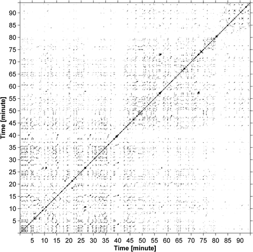
Exemplarily for the 12 investigated matches, Figure 4 shows the RP of a match which resulted in a 0–0 draw. Basically, three different blocks can be recognized in the RP separated by more-or-less white bands. The first block starts with the kick off and lasts until about minute 35. The second block starts at about minute 42 and ends at about minute 80. Finally, the last few minutes of the match form the third block. The gap between the first two blocks occurred because there was a sequence of longer game interruptions. In contrast to the first block, the match only ran for some seconds between the interruptions. They were free kicks at different locations on the pitch, a corner kick and a goal kick, all executed by the same team. The last 10 min of the match, the crunch time, were characterized by many interruptions accompanied by some yellow cards (four of five in this match) and two substitutions. Between those interruptions there were only short running match phases. Therefore, at the end of the match the pattern of the players differed from the other identified blocks. In particular, the first and the last blocks were different from each other. Inspecting the video of this match, a reason for this could be that the teams fulfilled precise tactical tasks at the beginning of the match whereas they behaved in a less ordered manner at the end of the match, when the home team tried to score in order to win the game by all available means. Another reason for this could be that the players were fatigued at the end of a match and usually ran shorter distances and less quickly during the final minutes [47,48].

Figure 4. Recurrence plot of one of the investigated matches (result 0–0; m = 1, tau = 1, ε = 9); black dots represent recurring states.

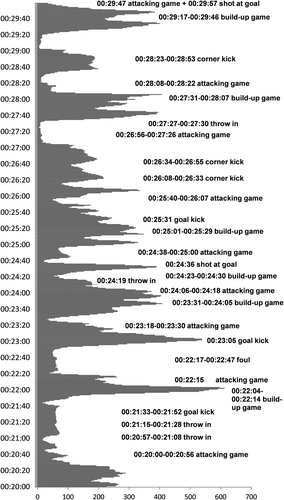
Because the analysis above suggests that the structure of RPs might be influenced by game interruptions, a detailed analysis of the recurrence points per second was conducted. For reasons of effort, three matches of the data set were selected and in each match 20 randomly chosen minutes were observed. Figure 5 shows the number of recurrence points per second and the respective discrete states (build-up game, attacking game, throw-in, corner kick, goal shot, etc.) of the game from above for a snippet of 10 min. Generally, the graph suggests that there were more recurrence points per second during open play phases (build-up game and attacking game) than during set pieces (corner kick, free kick, goal kick and throw-in). A t-test based on the sample of the three matches supports this assumption (open play: mean = 182.4, SD = 167.8; set-play: mean = 106.2, SD = 107.6; p < .001). This means that the teams showed similar patterns during open play phases more often. This could be due to several reasons. First of all, soccer matches are usually interrupted for fewer minutes than they are running [49]. Additionally, there are a lot of different reasons for set pieces, in particular free kicks, corner kicks and throw-ins, which take place at different locations on the field of play and cause different player patterns. Thus, it is obvious that there are fewer states set pieces can be similar to, and that there are fewer recurrence points during set pieces. Another reason why there were more recurrence points during open play could be related to the data set the study is based on. It consists of home games of a team which was one of the best teams in that season and which played quite dominantly. This probably biases the results towards the behaviour of this team. Moreover, the team’s playing style was characterized by long phases of ball possession during which the players were constrained to keep their tactical playing positions as unchanged as possible. Thus, the defending teams’ patterns also remained quite stable during such phases.

Figure 5. Recurrence points per second from one of the matches of the data set (result 0–0); discrete game phases are annotated.

RQAs were conducted to analyse the small-scale textures of the investigated RPs. RR was 2.3% on average (SD = 0.6). Thus, there were a lot of different states and only a few of them were similar to each other. Although DET was 96.3% on average (SD = 0.4%) and LAM was 98.4% (SD = 0.2%) on average, the diagonal lines (L = 5.5, SD = 0.3) and vertical lines (TT = 6.4, SD = 0.3) were not very long on average. The RQA parameter DET suggests that the progress of the match was rather predictable. However, considering L the match could only be predicted for a few seconds. Considering TT there were stable states which were repeatedly approached during matches. However, this could be an artefact caused by the recurrence threshold of 9 m together with the match’s velocity. For instance, if nearly all players were moving slowly it would have taken a few seconds until every player had moved further than 9 m. In particular, the matches reached such phases when the dominant team was attacking and trying to find an opening while the defending team was well organized.

Finally, the RQA parameters were correlated with a few game statistics from the investigated matches (Table 1). Only for a few correlations, significant results were found. The covered distances of the teams were moderately to strongly correlated with TT. This was surprising since the more the players move during 90 min the faster the match could be and the less time the players stay at similar locations. Furthermore, the number of goals in a match seemed to influence the RP structure, the more goals were scored the less structured was the match. Although the number of recurrence points is not correlated with the number of goals, DET and LAM significantly decreased when more goals were scored. Finally, there was a tendency that the more shots on goal there were in a match the fewer recurring states existed. This allowed us to assume that goal shots were probably not results of repeatedly performed, practised passing sequences.

Table 1. Pearson correlations between the game statistics number of goal shots, number of goals, number of corner kicks, number of fouls and covered distances of all players during a match and the RQA parameters RR, DET, L, LAM and TT of all investigated games.

	RR	DET	L	LAM	TT
Goal shots	−.56 (p = .056)	−.39 (p = .206)	.12 (p = .703)	−.40 (p = .201)	−.47 (p = .122)
Goals	.09 (p = .782)	−.63 (p = .028)	−.46 (p = .134)	−.61 (p = .034)	−.43 (p = .162)
Corner kicks	−.46 (p = .130)	.03 (p = .925)	.23 (p = .469)	.08 (p = .800)	−.14 (p = .671)
Fouls	−.22 (p = .498)	.34 (p = .284)	.40 (p = .201)	.41 (p = .189)	.45 (p = .141)
Covered distance	−.49 (p = .108)	−.42 (p = .169)	−.34 (p = .282)	−.48 (p = .119)	−.69 (p = .013)

Concluding, RP and RQA can be useful methods to analyse the dynamic, complex system soccer match. Using a more heterogeneous data set, the resulting RPs could help to shed light on the structure of soccer matches. In particular, investigating the RPs and their structure prior to important game actions such as goal shots or goals is an obvious question that should be approached. Furthermore, RPs should be analysed with respect to their potential regarding identifying and analysing tactical behaviour.

Conclusion

The complex, dynamic systems approach is frequently used in sports to model competitions or athletes. This paper illustrates how RPs – a tool frequently used in physics or earth science – can be applied to, and subsequently used, to analyse complex, dynamic sport systems. The application of the tool depends on the investigated sport. If a system is composed of a lot of unknown and not measureable parts, according to our case study a summary variable could be determined which describes the synergy of the components and is measurable. Based on such a measurement, the phase space reconstruction technique should be used for the RP construction to unfold hidden facets of a system’s dynamic. If several systems of the same type – such as golfers – are investigated, we recommend using the same phase space reconstruction. On the other hand, if there are many known and measureable parts a complex game sport system is composed of, the behaviour of those components should be measured and subsequently used as a multidimensional description of the system’s behaviour. We propose that such a detailed knowledge of the system’s behaviour does not require phase space reconstruction for the RP computation.

The choice of the recurrence threshold according to which states are assessed as similar is crucial because it determines how much information can be derived from the resulting RPs. Its determination depends on various factors such as whether there are several systems which are going to be compared in the context of sport scientific analyses. It is therefore recommended to use the same threshold for the different game sport systems under investigation. Using the average of the individual system’s thresholds turned out to be an appropriate choice.

The application of RPs to game sports allows a comprehensive view on sports performance, in particular its development over time. In particular, RQAs can help to shed light on the sporting performance of teams and individuals and can assist in answering sport scientific questions.

Acknowledgements

The authors would like to thank the PGA Tour for providing access to the ShotLink^TM database.

Disclosure statement

No potential conflict of interest was reported by the authors.

Additional information

Funding

This research was not supported by any grants.

References

- M. Hughes and I. Franks, Analysis of passing sequences, shots and goals in soccer, J. Sports Sci. 23 (2005), pp. 509–514. doi:10.1080/02640410410001716779
- L. Bishop and A. Barnes, Performance indicators that discriminate winning and losing in the knockout stages of the 2011 Rugby World Cup, Int. J. Perform. Anal. Sport. 13 (2013), pp. 149–159.
- P. O’Donoghue, Break points in Grand Slam men’s singles tennis, Int. J. Perform. Anal. Sport. 12 (2012), pp. 156–165.
- A. Redwood-Brown, Passing patterns before and after goal scoring in FA Premier League Soccer, Int. J. Perform. Anal. Sport. 8 (2008), pp. 172–182.
- P.S. Glazier, Game, set and match? Substantive issues and future directions in performance analysis, Sports Med. 40 (2010), pp. 625–634. doi:10.2165/11534970-000000000-00000
- R. Mackenzie and C. Cushion, Performance analysis in football: A critical review and implications for future research, J. Sports Sci. 31 (2013), pp. 639–676. doi:10.1080/02640414.2012.746720
- G. Mayer-Kress, Y.-T. Liu, and K.M. Newell, Complex systems and human movement, Complexity 12 (2006), pp. 40–51. doi:10.1002/(ISSN)1099-0526
- K. Davids, R. Shuttleworth, and C. Button, Acquiring skill in sport: A constraints led perspective, Int. J. Comp. Sci. Sport. 2 (2003), pp. 31–39.
- J.A.S. Kelso, Dynamic Patterns: The Self-Organization of Brain and Behavior, MIT press, Camebridge, MA, 1997.
- J.-F. Grehaigne, D. Bouthier, and B. David, Dynamic-system analysis of opponent relationships in collective actions in soccer, J. Sports Sci. 15 (1997), pp. 137–149. doi:10.1080/026404197367416
- T. McGarry, D.I. Anderson, S. Wallace, M. Hughes, and I.M. Franks, Sport competition as a dynamical self-organizing system, J. Sports Sci. 20 (2002), pp. 771–781. doi:10.1080/026404102320675620
- H. Haken, Synergetics. An Introduction. Nonequilibrium Phase Transitions and Self-Organization in Physics, Chemistry, and Biology, Springer, Berlin, 1977.
- J.J. Gibson, The theory of affordances, in Perceiving, Acting, and Knowing: Toward an Ecological Psychology, R.E. Shaw and J. Bransford, eds., Lawrence Erlbaum Associates, Hillsdale, 1977, pp. 67–82.
- K.M. Newell, Constraints on the development of coordination, Motor dev. children Aspects coord. control. 34 (1986), pp. 341–360.
- F. Walter, M. Lames, and T. McGarry, Analysis of sports performance as a dynamical system by means of the relative phase, Int. J. Comp. Sci. Sport. 6 (2007), pp. 35–41.
- Y. Palut and P.-G. Zanone, A dynamical analysis of tennis: Concepts and data, J. Sports Sci. 23 (2005), pp. 1021–1032. doi:10.1080/02640410400021682
- H. Folgado, R. Duarte, O. Fernandes, and J. Sampaio, Competing with lower level opponents decreases intra-team movement synchronization and time-motion demands during pre-season soccer matches, PLoS ONE 9 (2014), pp. e97145. doi:10.1371/journal.pone.0097145
- M. Siegle and M. Lames, Modeling soccer by means of relative phase, J. Syst. Sci. Complex 26 (2013), pp. 14–20. doi:10.1007/s11424-013-2283-2
- J. Bourbousson, C. Sève, and T. McGarry, Space–time coordination dynamics in basketball: Part 1. Intra-and inter-couplings among player dyads, J. Sports Sci. 28 (2010), pp. 339–347. doi:10.1080/02640410903503632
- J. Bourbousson, C. Sève, and T. McGarry, Space–time coordination dynamics in basketball: Part 2. The interaction between the two teams, J. Sports Sci. 28 (2010), pp. 349–358. doi:10.1080/02640410903503640
- S. Fonseca, J. Milho, P. Passos, D. Araujo, and K. Davids, Approximate entropy normalized measures for analyzing social neurobiological systems, J. Mot. Behav. 44 (2012), pp. 179–183. doi:10.1080/00222895.2012.668233
- J. Sampaio and V. Maçãs, Measuring tactical behaviour in football, Int. J. Sports Med. 33 (2012), pp. 395–401. doi:10.1055/s-0031-1301320
- N. Marwan, M.C. Romano, M. Thiel, and J. Kurths, Recurrence plots for the analysis of complex systems, Phys. Rep. 438 (2007), pp. 237–329. doi:10.1016/j.physrep.2006.11.001
- J. Carvalho, D. Araújo, B. Travassos, P.T. Esteves, L. Pessanha, F. Pereira, and K. Davids, Dynamics of players’ relative positioning during baseline rallies in tennis, J. Sports Sci. 31 (2013), pp. 1596–1605. doi:10.1080/02640414.2013.792944
- M.S. Magnusson, Discovering hidden time patterns in behavior: T-patterns and their detection, Behav. Res. Methods Instrum. Comput. 32 (2000), pp. 93–110. doi:10.3758/BF03200792
- G.K. Jonsson, M. Anguera, P. Sánchez-Algarra, C. Olivera, J. Campanico, M. Castañer, and J. Chaverri, Application of T-pattern detection and analysis in sports research, Open Sports Sci. J. 3 (2010), pp. 95–104. doi:10.2174/1875399X010030100095
- M. Broadie, Assessing golfer performance on the PGA TOUR, Interfaces 42 (2012), pp. 146–165. doi:10.1287/inte.1120.0626
- M. Stöckl, P.F. Lamb, and M. Lames, A model for visualizing difficulty in golf and subsequent performance rankings on the PGA tour, Int. J Golf Sci. 1 (2012), pp. 10–24. doi:10.1123/ijgs.1.1.10
- M. Bar-Eli, S. Avugos, and M. Raab, Twenty years of “hot hand” research: Review and critique, Psychol. Sport. Exerc. 7 (2006), pp. 525–553. doi:10.1016/j.psychsport.2006.03.001
- R.D. Clark III, An examination of the hot hand in professional golfers, Percept. Mot. Skills 101 (2005), pp. 935–942. doi:10.2466/pms.101.3.935-942
- N. James, The statistical analysis of golf performance, Int. J of Sports Sci & Coaching 2 (2007), pp. 231–248.
- J.A. Livingston, The hot hand and the cold hand in professional golf, J. Econ. Behav. Organ. 81 (2012), pp. 172–184. doi:10.1016/j.jebo.2011.10.001
- J.-P. Eckmann, S. Oliffson Kamphorst, and D. Ruelle, Recurrence plots of dynamical systems, World Sci. Ser. Nonlinear Sci. Ser. 16 (1995), pp. 441–446.
- F. Takens, Detecting Strange Attractors in Turbulence, Springer, Berlin Heidelberg, 1981.
- J.S. Iwanski and E. Bradley, Recurrence plots of experimental data: To embed or not to embed? Chaos 8 (1998), pp. 861–871. doi:10.1063/1.166372
- J. Gao and H. Cai, On the structures and quantification of recurrence plots, Phys. Lett. A 270 (2000), pp. 75–87. doi:10.1016/S0375-9601(00)00304-2
- M.B. Kennel, R. Brown, and H.D.I. Abarbanel, Determining embedding dimension for phase-space reconstruction using a geometrical construction, Phys. Rev. 45 (1992), pp. 3403–3411. doi:10.1103/PhysRevA.45.3403
- N. Marwan and C.L. Webber Jr., Mathematical and computational foundations of recurrence quantifications, in Recurrence Quantification Analysis: theory and Best Practices, C.L. Webber Jr. and N. Marwan, eds., Springer International Publishing, New York, 2014, pp. 3–43.
- T.K. March, S.C. Chapman, and R.O. Dendy, Recurrence plot statistics and the effect of embedding, Physica D 200 (2005), pp. 171–184. doi:10.1016/j.physd.2004.11.002
- G.M. Mindlin and R. Gilmore, Topological analysis and synthesis of chaotic time series, Physica D 58 (1992), pp. 229–242. doi:10.1016/0167-2789(92)90111-Y
- M. Koebbe and G. Mayer-Kress, Use of recurrence plots in the analysis of time-series data, Santa Fe Inst. Stud. Sci. Complexity-Proceedings. 12 (1992), pp. 361.
- N. Marwan, Untersuchung der Klimavariabilität in NW Argentinien mit Hilfe der quantitativen Analyse von Recurrence Plots, Master Thesis, TU Dresden, 1999.
- J.P. Zbilut, N. Thomasson, and C.L. Webber, Recurrence quantification analysis as a tool for nonlinear exploration of nonstationary cardiac signals, Med. Eng. Phys. 24 (2002), pp. 53–60. doi:10.1016/S1350-4533(01)00112-6
- N. James, Performance analysis of golf: Reflections on the past and a vision of the future, Int. J. Perform. Anal. Sport. 9 (2009), pp. 188–209.
- NIST/SEMATECH, e-Handbook of statistical methods, Available at http://www.itl.nist.gov/div898/handbook/.
- C.L. Webber and J.P. Zbilut, Recurrence quantifications: Feature extractions from recurrence plots, Int. J. Bifurcat. Chaos. 17 (2007), pp. 3467–3475. doi:10.1142/S0218127407019226
- M. Mohr, P. Krustrup, and J. Bangsbo, Match performance of high-standard soccer players with special reference to development of fatigue, J. Sports Sci. 21 (2003), pp. 519–528. doi:10.1080/0264041031000071182
- R. Akenhead, P.R. Hayes, K.G. Thompson, and D. French, Diminutions of acceleration and deceleration output during professional football match play, J. Sci. Med. Sport 16 (2013), pp. 556–561. doi:10.1016/j.jsams.2012.12.005
- M. Siegle and M. Lames, Game interruptions in elite soccer, J. Sports Sci. 30 (2012), pp. 619–624. doi:10.1080/02640414.2012.667877