Modelling and identification of nonlinear cascade systems with backlash input and static output nonlinearities

ABSTRACT

A new approach to the parameter identification of nonlinear dynamic systems using cascade models with nonlinear dynamic, linear dynamic and nonlinear static blocks is presented. Application of the key-term separation principle provides special expressions for the corresponding nonlinear model description that are linear in parameters. A least-squares-based iterative technique is proposed allowing estimation of all the model parameters based on measured input/output data. Illustrative examples of nonlinear cascade systems identification with input backlash and nonlinear static output characteristics are included.

KEYWORDS:

• Nonlinear system
• system modelling
• parameter estimation
• computer simulation
• cascade models
• backlash

Introduction

Identification of nonlinear dynamic systems is a very specific problem, because we are not able to propose a universal approach to all existing systems. As the system identification is always based on appropriate mathematical models, it is almost impossible to propose a class of universal mathematical models describing efficiently all nonlinear dynamic systems. Therefore, the model choice is often oriented to practical but sufficiently broad classes of model structures.

One way to specify nonlinear dynamic model structure is to combine linear dynamic submodels with nonlinear static (memoryless) submodels or blocks. These nonlinear models are called block-oriented models and there are several advantages for using them in the system identification, because it is easy to comprehend, to incorporate a priori process knowledge, and to use them in control. Commonly used block-oriented models are the so-called Hammerstein model, Wiener model and their combinations. The Hammerstein model consists of a nonlinear static block followed by a linear dynamic block and many researchers have studied the identification of nonlinear dynamic systems using Hammerstein model. The identification techniques mainly distinguish themselves in the way the static nonlinearity is represented and in the type of optimization problem that is finally obtained. Known approaches for different types of nonlinearities include gradient methods [1–3], recursive methods [4–6], iterative methods [7–9] and more special approaches e.g. [10,11]. The Wiener model has a linear dynamic block followed by a nonlinear static block and lots of techniques have been proposed to solve the optimization problems typically encountered in using this model including iterative methods [12–15], nonparametric methods [16,17] and special approaches e.g. [18–22].

More complex nonlinear dynamic systems can be modelled by putting more block-oriented models in series. One of them is the Hammerstein–Wiener model that consists of a linear dynamic block embedded between two static nonlinear blocks. In control systems, the use of this model is motivated by considering the input nonlinear block as actuator nonlinearity and the output nonlinear block as process nonlinearity or sensor nonlinearity. More identification approaches are using this model; see e.g. [23–29]. Note that the nonlinear blocks of Hammerstein model, Wiener model and their combinations are assumed static, i.e. without memory. Unfortunately, none of the above-mentioned block-oriented models can be used if nonsmooth dynamic nonlinearities exist in control systems.

Nonsmooth nonlinearities, such as hysteresis or backlash, often occur in real process control, due to physical, technological or safety constraints, imperfections, or even inherent characteristics of considered controlled systems [30]. They are common in components of many control systems, such as actuators of servo control systems, mechanical transmission systems, and hydraulic control valves. A wide variety of practical systems and devices may then be represented by the cascade of a non-smooth nonlinear operator and the rest of given system.

Backlash is one of the most important nonlinearities that strongly affect the chosen control strategies in industrial processes and its presence gives rise to inaccuracies in the position and velocity. This nonlinearity, which can be classified as a dynamic (i.e. with memory) and hard (i.e. non-differentiable) one, commonly occurs in mechanical, hydraulic and other components, e.g. bearings, gears. The backlash can arise from unavoidable manufacturing tolerances or sometimes can be deliberately incorporated in the system in order to cope with thermal expansion.

Disregard of input backlash will worsen the system performance and even lead to serious instability; therefore, the identification of systems with backlash is of great importance. More approaches were presented on identification of two-block cascade systems with input backlash followed by a linear dynamic subsystem [31–39]. However, up to now no results were published on the identification of cascade systems with dynamic input and static output nonlinearities.

In this paper, a new class of cascade models for systems with input (actuator) backlash and static output (sensor) nonlinearity is introduced. The fundamental difference between the proposed cascade models and those of [40] is that in this case, a nonlinear dynamic block (backlash) is followed by a linear dynamic block and this is followed by a nonlinear static block. Inclusion of the nonlinear output block significantly influences the structure of resulting block-oriented model and determines a new class of nonlinear mathematical models being linear in parameters. The proposed models are appropriate for precise modelling of nonlinear dynamics of actuators and the static nonlinearities of sensors in control systems especially in robotics. To the best knowledge of the author of this paper, no approach has been reported on modelling and identification of this type of nonlinear dynamic systems.

The paper is organized as follows. First, a new class of three-block cascade models is introduced. Then the so-called key-term separation principle [9,15] is applied to simplify the form of proposed mathematical models and make them linear in parameters. The resulting model equation is without cross-multiplication of parameters; nevertheless, it contains more internal variables, which are generally unmeasurable, therefore an iterative parameter estimation approach is proposed. This enables, on the basis of measured input/output data, the estimation of all the model parameters as well as all internal variables. It means that the internal variables are repeatedly recomputed using the recent parameters estimates and then used for the parameter estimation in the next iteration minimizing the least-squares criterion.

Illustrative examples of nonlinear dynamic systems identification with backlash in the input nonlinear block and nonlinear static characteristics in the output block are included to show the effectiveness of the proposed algorithm. Finally, some concluding remarks are offered.

Model description

Assume that the nonlinear dynamic system can be modelled by the serial connection of a nonlinear dynamic block with backlash followed by a linear dynamic block, which is followed by a nonlinear static block according to Figure 1.

Figure 1. Three-block cascade system with input backlash.

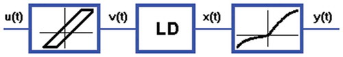
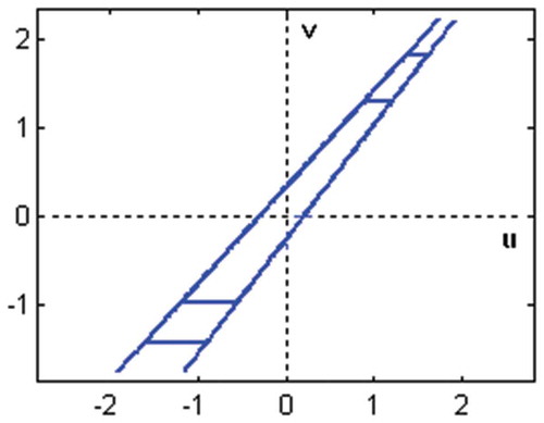
The input backlash characteristic with input u(t) and output v(t) is described by two straight lines, upward (right) and downward (left) sides of backlash, connected with horizontal line segments [31]. The backlash nonlinearity is shown in Figure 2, and the mathematical model for the discrete-time case is given by

(1) $v(t)=\left\{\begin{array}{cc}{m}_L[u(t)+c_L]& u(t)\le z_L\\ m_R[u(t)-c_R]& u(t)\ge z_R\\ v(t-1)& z_L\le u(t)\le z_R\end{array}\right.$(1)

Figure 2. Input backlash.

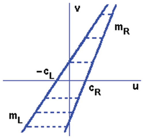
where t = 1, 2, 3, …, m_L, m_R, c_L > 0, c_R > 0 are constant parameters characterizing the backlash and

(2) $z_L=\frac{v(t-1)}{m_L}-c_L$(2)

(3) $z_R=\frac{v(t-1)}{m_R}+c_R$(3)

are the u-axis values of intersections of the two lines, with slopes m_L, m_R, with the horizontal inner segment containing v(t – 1). The slopes of straight lines m_L and m_R may be simultaneously positive or negative, while c_L and c_R must be positive. This model allows the upward and downward line slopes to be different if the intersection of the two lines is not in the region of practical interest.

The backlash model can be described by the following first-order difference equation [37]:

(4) $v(t)=m_{L}u(t)f_1(t)+m_L{c}_L{f}_1(t)+m_{R}u(t)f_2(t)-m_R{c}_R{f}_2(t)+v(t-1)[1-f_1(t)][1-f_2(t)]$(4)

where

(5) $f_1(t)=h[u(t)-z_L]=h\left\{[m_{L}u(t)+m_L{c}_L-v(t-1)]/m_L\right\}$(5)

(6) $f_2(t)=h[z_R-u(t)]=h\left\{[v(t-1)-m_{R}u(t)+m_R{c}_R]/m_R\right\}$(6)

are internal variables based on (2) and (3) using the following function:

(7) $h(\sigma )=\left\{\begin{array}{c}0,if\sigma >0\\ 1,if\sigma \le 0\end{array}\right.$(7)

switching between two sets of values, i.e. (– ∞, σ) and (σ, ∞). The input/output relation (4) is identical with that of (1).

Let the linear dynamic block of the three-block cascade model consists of a linear time-invariant dynamic system. Then the input/output relation in the time domain for the linear dynamic block can be given by the following difference equation:

(8) $x(t)=\sum _{i=1}^r{a}_{i}v(t-i)-\sum _{j=1}^p{b}_{j}x(t-j).$(8)

where v(t) and x(t) are the inputs and outputs, respectively.

The input/output relation of the output static block can be written as

(9) $y(t)=g(x(t)).$(9)

and we assume that the nonlinear map g(.) can be described by a linear combination of a known basis ξ(x(t)) = (ξ₁(x(t)), ξ₂(x(t)), …, ξ_n(x(t))) with coefficients (g₁, g₂, …, g_n) as

(10) $g(x(t))=\sum _{k=1}^n{g}_k{\xi }_k(x(t))$(10)

and the basis functions can be splines, polynomial, trigonometric, piecewise linear functions.

The description (10) can be generalized for the case when the outputs of nonlinear static block y(t) significantly depend on the sign of inputs x(t). Let the output nonlinear static block be described by two nonlinear functions [9]

(11) $y(t)=\left\{\begin{array}{c}\alpha (x(t))\mathrm{i}\mathrm{f}x(t)\ge 0\\ \beta (x(t))\mathrm{i}\mathrm{f}x(t)<0\end{array}\right.$(11)

Then the relation between the inputs and outputs of this static block can be written as follows:

(12) $y(t)=\alpha (x(t))+(\beta (x(t))-\alpha (x(t)))h(x(t)).$(12)

Assume the nonlinear maps α(.) and β(.) can be described by a linear combination of a known basis ξ(x(t)) = (ξ₁(x(t)), ξ₂(x(t)), …, ξ_n(x(t))) with coefficients (α₁, α₂, …, α_n) and (β₁, β₂, …, β_n) as follows:

(13) $\alpha (x(t))=\sum _{k=1}^n{\alpha }_k{\xi }_k(x(t))$(13)

(14) $\beta (x(t))=\sum _{k=1}^n{\beta }_k{\xi }_k(x(t))$(14)

Then the nonlinear static block with two-segment nonlinearity can be described by the following equation:

(15) $y(t)=\sum _{k=1}^n{\alpha }_k{\xi }_k(x(t))+\sum _{k=1}^n{\gamma }_k{\xi }_k(x(t))h(x(t))+e(t)$(15)

where γ_k = β_k – α_k, e(t) is the measurement noise and the basis functions can be splines, polynomial, trigonometric, piecewise linear functions.

Assume that the linear dynamic subsystem is stable, the base functions are polynomials, i.e. ξ_i(x(t)) = xⁱ(t), the degrees r, p and n are known and y(t) = 0, u(t) = 0, x(t) = 0 and v(t) = 0 for t ≤ 0. Then the three-block cascade model description can be created by consecutive substitutions of (4) into (8) and then the result of this substitution into (15). However, this will result in a very complex equation with cross-multiplications of parameters. Therefore, the so-called key-term separation principle [9,15] will be applied to transform the system described by Equations (4), (8) and (15) into a pseudo-linear representation without the products of parameters.

Note that the parameterization of the cascade connection of three blocks is not unique, as many combinations of parameters can be found. If the three-block system in Figure 1 is represented e.g. by v = g(u), x = L(q⁻¹)v and y = f(x), then, any triple ag(u), bL(q⁻¹) and cf(x), for some constants a, b, c such that abc = 1, would provide the same input–output data. Strictly speaking, no identification setting can distinguish between (g; L; f) and (ag; bL; cf). To obtain a unique parameterization, two blocks need to be normalised. For application of the key term separation principle, it is appropriate to normalize the linear block and the output nonlinearity by choosing a₁ = 1, and α₁ = 1.

To construct the input/output equation of the cascade model, we separate the first term in the description the linear dynamic block as follows:

(16) $x(t)=v(t-1)+\sum _{i=2}^r{a}_{i}v(t-i)-\sum _{j=1}^p{b}_{j}x(t-j)$(16)

and then we half-substitute (4) into (16), i.e. only for the separated term

(17) $\begin{array}{rl}& x(t)=m_{L}u(t-1)f_1(t-1)+m_L{c}_L{f}_1(t-1)+m_{R}u(t-1)f_2(t-1)-m_R{c}_R{f}_2(t-1)+\\ & +v(t-2)[1-f_1(t-1)][1-f_2(t-1)]+\sum _{i=2}^r{a}_{i}v(t-i)-\sum _{j=1}^p{b}_{j}x(t-j)\end{array}$(17)

Finally, the output equation of this cascade model can be constructed by half-substituting (17) into (15), i.e. only for the first term in the description of output block, as follows:

(18) $\begin{array}{rl}& y(t)=m_{L}u(t-1)f_1(t-1)+m_L{c}_L{f}_1(t-1)+m_{R}u(t-1)f_2(t-1)-m_R{c}_R{f}_2(t-1)+\\ & +v(t-2)[1-f_1(t-1)][1-f_2(t-1)]+\sum _{i=2}^r{a}_{i}v(t-i)-\sum _{j=1}^p{b}_{j}x(t-j)\\ & +\sum _{k=2}^n{\alpha }_k{x}^k(t)+\sum _{k=1}^n{\gamma }_k{x}^k(t)h(x(t))+e(t)\end{array}$(18)

with

(19) $m_L=m_1,c_L=c_1/m_1,m_R=m_2,c_R=c_2/m_2,$(19)

where the parameters of the input backlash, the linear dynamic block and the output nonlinearity are separated and the equation is quasi-linear as the internal variables f₁(t) and f₂(t) depend on the backlash parameters.

Parameter estimation

The input/output Equation (18) can be used for estimation of model parameters. Defining the following vector of data:

(20) $\begin{array}{rl}& \varphi (t)=[u(t-1)f_1(t-1),f_1(t-1),u(t-1)f_2(t-1),-f_2(t-1),v(t-2),\cdots ,v(t-r),\\ & -x(t-1),\cdots ,-x(t-p),x^2(t),\cdots ,x^n(t),x(t)h(x(t)),\cdots ,x^n(t)h(x(t)){]}^T\end{array}$(20)

and the parameter vector

(21) $\theta =[m_1,c_1,m_2,c_2,a_2,\cdots ,a_r,b_1,\cdots ,b_p,{\alpha }_2,\cdots ,{\alpha }_n,{\gamma }_1,\cdots ,{\gamma }_n{]}^T$(21)

the three-block cascade model can be written in the following form:

(22) $y_c(t)=y(t)-v(t-2)[1-f_1(t-1)][1-f_2(t-1)]={\varphi }^T(t)\theta +e(t)$(22)

Considering N observations of input u(t) and output y(t) and assuming that u(t) = 0 and y(t) = 0 for t ≤ 0, we can define the stacked corrected output vector Y_c(N), the stacked information matrix Φ(N) and the stacked noise vector E(N) as follows:

(23) $Y_c(N)=\left[\begin{array}{c}{y}_c(1)\\ y_c(2)\\ :\\ y_c(N)\end{array}\right]$(23)

(24) $\mathrm{\Phi }(N)=\left[\begin{array}{c}\varphi (1)\\ \varphi (2)\\ :\\ \varphi (N)\end{array}\right]$(24)

(25) $E(N)=\left[\begin{array}{c}e(1)\\ e(2)\\ :\\ e(N)\end{array}\right]$(25)

then from (22), we have

(26) $Y_c(N)=\mathrm{\Phi }(N)\theta +E(N)$(26)

Minimizing the least-squares criterion function

(27) $J(\theta )={∥Y_c(N)-\mathrm{\Phi }(N)\theta ∥}^2$(27)

with respect to θ and assuming that the information matrix Φ(N) is persistently exciting, that is, Φ^T(N)Φ(N) is an invertible matrix, we can obtain the least-squares estimate of the parameter vector as follows:

(28) $\hat{\theta }=[{\mathrm{\Phi }}^T(N)\mathrm{\Phi }(N){]}^{-1}{\mathrm{\Phi }}^T(N)Y_c(N)$(28)

However, the information matrix Φ(N) and the corrected output vector Y_c(N) contain unknown internal variables; therefore, an iterative algorithm must be applied for estimation of model parameters.

The technique presented in [36–38], which is based on the use of the preceding estimates of model parameters for the estimation of internal variables and vice-versa, can be easily extended to this three-block model. We replace the internal variables and the corrected output in sth iteration by their estimates

(29) ${ }^{s}v(t)={\hspace{0.17em}}_{\hspace{0.17em}}^s{m}_{1}u(t){\hspace{0.17em}}_{\hspace{0.17em}}^s{f}_1(t)+{\hspace{0.17em}}_{\hspace{0.17em}}^s{c}_1{\hspace{0.17em}}_{\hspace{0.17em}}^s{f}_1(t)+{\hspace{0.17em}}_{\hspace{0.17em}}^s{m}_{2}u(t){\hspace{0.17em}}_{\hspace{0.17em}}^s{f}_2(t)-{\hspace{0.17em}}_{\hspace{0.17em}}^s{c}_2{\hspace{0.17em}}_{\hspace{0.17em}}^s{f}_2(t)+{\hspace{0.17em}}_{\hspace{0.17em}}^{s}v(t-1)[1-{\hspace{0.17em}}_{\hspace{0.17em}}^s{f}_1(t)][1-{\hspace{0.17em}}_{\hspace{0.17em}}^s{f}_2(t)]$(29)

(30) ${ }^s{m}_L={\hspace{0.17em}}_{\hspace{0.17em}}^s{m}_1,{\hspace{0.17em}}_{\hspace{0.17em}}^s{c}_L={\hspace{0.17em}}_{\hspace{0.17em}}^s{c}_1/{\hspace{0.17em}}_{\hspace{0.17em}}^s{m}_1,{\hspace{0.17em}}_{\hspace{0.17em}}^s{m}_R={\hspace{0.17em}}_{\hspace{0.17em}}^s{m}_2,{\hspace{0.17em}}_{\hspace{0.17em}}^s{c}_R={\hspace{0.17em}}_{\hspace{0.17em}}^s{c}_2/{\hspace{0.17em}}_{\hspace{0.17em}}^s{m}_2,$(30)

(31) ${ }^s{f}_1(t)=h\left\{[{\hspace{0.17em}}_{\hspace{0.17em}}^s{m}_{L}u(t)+{\hspace{0.17em}}_{\hspace{0.17em}}^s{m}_L{\hspace{0.17em}}_{\hspace{0.17em}}^s{c}_L-{\hspace{0.17em}}_{\hspace{0.17em}}^{s}v(t-1)]/{\hspace{0.17em}}_{\hspace{0.17em}}^s{m}_L\right\}$(31)

(32) ${ }^s{f}_2(t)=h\left\{[{\hspace{0.17em}}_{\hspace{0.17em}}^{s}v(t-1)-{\hspace{0.17em}}_{\hspace{0.17em}}^s{m}_{R}u(t)+{\hspace{0.17em}}_{\hspace{0.17em}}^s{m}_R{\hspace{0.17em}}_{\hspace{0.17em}}^s{c}_R]/{\hspace{0.17em}}_{\hspace{0.17em}}^s{m}_R\right\}$(32)

(33) ${ }^{s}x(t)={\hspace{0.17em}}_{\hspace{0.17em}}^{s}v(t-1)+\sum _{i=2}^r{\hspace{0.17em}}_{\hspace{0.17em}}^s{a}_i{\hspace{0.17em}}_{\hspace{0.17em}}^{s}v(t-i)-\sum _{j=1}^p{\hspace{0.17em}}_{\hspace{0.17em}}^s{b}_j{\hspace{0.17em}}_{\hspace{0.17em}}^{s}x(t-j)$(33)

(34) ${ }^s{y}_c(t)=y(t)-{\hspace{0.17em}}_{\hspace{0.17em}}^{s}v(t-2)[1-{\hspace{0.17em}}_{\hspace{0.17em}}^s{f}_1(t-1)][1-{\hspace{0.17em}}_{\hspace{0.17em}}^s{f}_2(t-1)]$(34)

Then defining the estimate of the data vector

(35) $\begin{array}{rl}& { }^s\varphi (t)=[u(t-1{)}^s{f}_1(t-1),{}^s{f}_1(t-1),u(t-1{)}^s{f}_2(t-1),{-}^s{f}_2(t-1){,}^{s}v(t-2),\cdots ,\\ & {}^{s}v(t-r),{-}^{s}x(t-1),\cdots ,{-}^{s}x(t-p){,}^s{x}^2(t),\cdots {,}^s{x}^n(t){,}^{s}x(t)h{(}^{s}x(t)),\cdots ,\\ & {}^s{x}^n(t)h{(}^{s}x(t)){]}^T\end{array}$(35)

and forming the corrected output vector ^sY_c(N) and the information matrix ^sΦ(N)

(36) ${\hspace{0.17em}}_{\hspace{0.17em}}^s{Y}_c(N)=\left[\begin{array}{c}{\hspace{0.17em}}_{\hspace{0.17em}}^s{y}_c(1)\\ {\hspace{0.17em}}_{\hspace{0.17em}}^s{y}_c(2)\\ :\\ {\hspace{0.17em}}_{\hspace{0.17em}}^s{y}_c(N)\end{array}\right]$(36)

(37) ${\hspace{0.17em}}_{\hspace{0.17em}}^s\mathrm{\Phi }(N)=\left[\begin{array}{c}{\hspace{0.17em}}_{\hspace{0.17em}}^s\varphi (1)\\ {\hspace{0.17em}}_{\hspace{0.17em}}^s\varphi (2)\\ :\\ {\hspace{0.17em}}_{\hspace{0.17em}}^s\varphi (N)\end{array}\right]$(37)

we will minimize the least-squares criterion function

(38) $J({\hspace{0.17em}}^{s+1}\theta )={∥{\hspace{0.17em}}^s{Y}_c(N)-{\hspace{0.17em}}^s\mathrm{\Phi }(N){\hspace{0.17em}}^{s+1}\theta ∥}^2$(38)

with respect to ^s+1θ giving

(39) ${\hspace{0.17em}}_{\hspace{0.17em}}^{s+1}\theta =[{\hspace{0.17em}}_{\hspace{0.17em}}^s{\mathrm{\Phi }}^T(N){\hspace{0.17em}}_{\hspace{0.17em}}^s\mathrm{\Phi }(N){]}^{-1}{\hspace{0.17em}}_{\hspace{0.17em}}^s{\mathrm{\Phi }}^T(N){\hspace{0.17em}}_{\hspace{0.17em}}^s{Y}_c(N)$(39)

If the input u(t) is persistently excited with respect to the dead zone of input backlash, the steps of the iterative procedure for the given set of input/output data {u(t); y(t)}, t = 1, 2, …. N, are listed as follows:

Step 1. For s = 1, set ¹v(t) = u(t) and ¹x(t) = y(t), consider nonzero initial values of backlash parameters (e.g. ¹m_L = ¹m_R = 1 for the backlash with positive slopes or ¹m_L = ¹m_R = – 1 for the backlash with negative slopes, while ¹c_L and ¹c_R are chosen small enough).

Step 2. Compute the estimates of internal variables using (29) – (33).

Step 3. Compute the estimates of corrected outputs using (34).

Step 4. Form the corrected output vector ^sY_c(N) and the information matrix ^sΦ(N) using (36) and (37).

Step 5. Update the parameter estimates ^s+1θ using (39).

Step 6. For some pre-set small δ, if J(^s+1θ) < δ, then the iterative procedure terminates otherwise, put s = s + 1 and go to Step 2.

Note, that only the linear dynamic block and output block parameters are estimated in the first iteration, if we choose very small ¹c_L and ¹c_R, i.e. actually a Wiener model approximation is considered.

Simulation studies

The proposed identification method for the identification of systems with input backlash and two-segment polynomial output nonlinearity was implemented and tested in MATLAB. Several cases were simulated and the estimations of parameters were carried out on the basis of input and output records. The performance of the proposed methods is illustrated on the following examples.

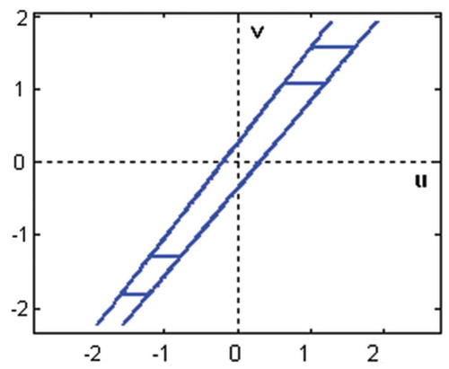
Example 1: The cascade system with an input backlash (Figure 3) characterized by the parameters m_L = 1.3, c_L = 0.3, m_R = 1.2, c_R = 0.2 and followed by the linear dynamic system described by the difference equation

$x(t)=v(t-1)+0.5v(t-2)+0.2x(t-1)-0.35x(t-2)$

Figure 3. Example 1 – input backlash.

and the following two-segment polynomial output:

$y(t)=\left\{\begin{array}{cc}x(t)-0.9x^2(t)+0.3x^3(t)& \mathrm{i}\mathrm{f}x(t)\ge 0\\ -0.1x^2(t)+0.1x^3(t)& \mathrm{i}\mathrm{f}x(t)<0\end{array}\right.$

was considered (Figure 4). The identification was performed on the basis of 4000 samples of uniformly distributed random inputs with |u(t)| < 2.0 and simulated outputs. Normally distributed random noise with zero mean and signal-to-noise ratio – SNR = 50 (the square root of the ratio of output and noise variances) was added to the outputs. The iterative estimation algorithm was applied with initial values m_L = m_R = 1 and c_L = c_R = 0.001 for the first estimate of f₁(t) and f₂(t), while the initial values of linear dynamic system and nonlinear static system parameters were chosen zero. The process of parameter estimation is shown in Figure 5 for the backlash, in Figure 6 for the linear block and in Figure 7 for the nonlinear block. The estimates meet the values of real parameters after about 15 iterations.

Figure 4. Example 1 – output nonlinearity.

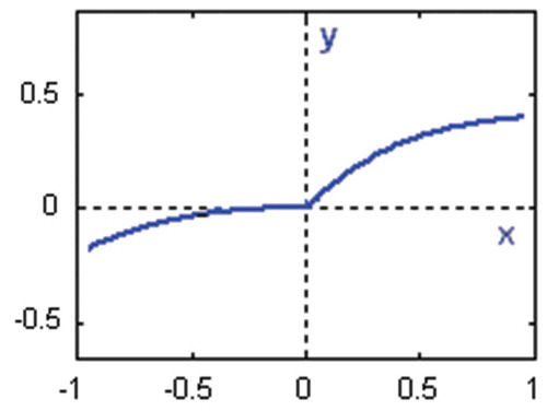
Figure 5. Example 1 – the process of parameter estimation for the backlash (the top–down order of parameters is m_L, m_R, c_L, c_R).

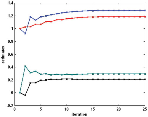
Figure 6. Example 1 – the process of parameter estimation for the linear dynamic block (the top–down order of parameters is a₂, b₂, b₁).

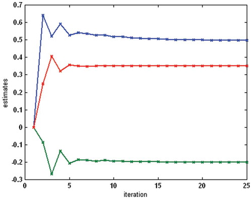
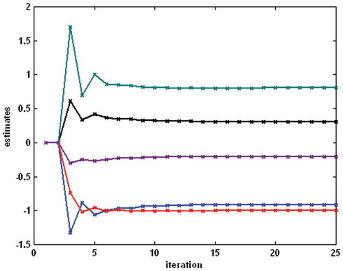
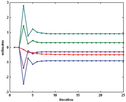
Figure 7. Example 1 – the process of parameter estimation for the nonlinear block (the top–down order of parameters is γ₂, α₃, γ₃, α₂, γ₁).

Example 2: The cascade system with an input backlash (Figure 8) characterized by the parameters m_L = 1.1, c_L = 0.3, m_R = 1.3, c_R = 0.2 and followed by the linear dynamic system described by the difference equation

$x(t)=v(t-1)+0.5v(t-2)+0.2x(t-1)-0.35x(t-2)$

Figure 8. Example 2 – input backlash.

and the following two-segment polynomial output:

$y(t)=\left\{\begin{array}{cc}x(t)-0.9x^2(t)+0.3x^3(t)& \mathrm{i}\mathrm{f}x(t)\ge 0\\ 0.5x(t)& \mathrm{i}\mathrm{f}x(t)<0\end{array}\right.$

was considered (Figure 9). The identification was performed under the same conditions as in Example 1. The process of parameter estimation is shown in Figure 10 for the backlash, in Figure 11 for the linear block and in Figure 12 for the nonlinear block. The estimates meet the values of real parameters after about 12 iterations.

Figure 9. Example 2 – output nonlinearity.

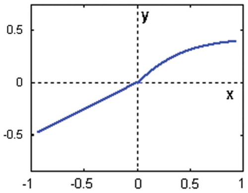
Figure 10. Example 2 – the process of parameter estimation for the backlash (the top–down order of parameters is m_R, m_L, c_L, c_R).

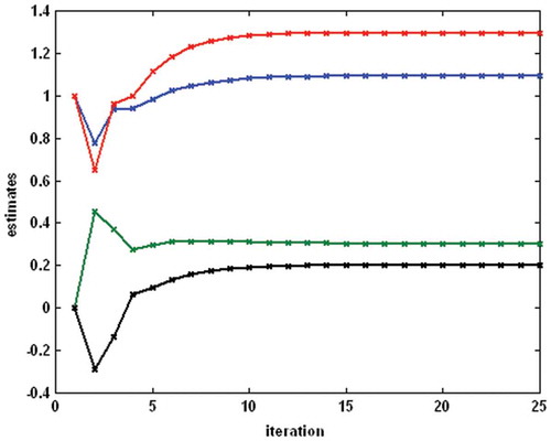
Figure 11. Example 2 – the process of parameter estimation for the linear dynamic block (the top–down order of parameters is a₂, b₂, b₁).

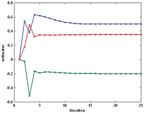
Figure 12. Example 2 – the process of parameter estimation for the nonlinear block (the top–down order of parameters is γ₂, α₃, γ₃, γ₁, α₂).

Note that although there exist proofs of convergence for iterative identification algorithms considering the cascade of nonlinear static, linear dynamic and nonlinear static blocks, unfortunately no proof of convergence exists for the presented cascade model. The main problem is with the nonlinear dynamic block with backlash, as a multivalued mapping. However, testing of the proposed algorithm and the above examples show that the convergence rate is relatively high despite the complex structure of proposed model and the additive output noise.

Conclusion

Backlash exists in a wide range of physical systems and devices and its identification is crucial for control purposes especially in the case of input backlash appearing in actuators. The presented approach to the identification of nonlinear cascade systems with backlash input and static output nonlinearities is based on the new class of nonlinear mathematical models being linear in parameters with input/output equation resulting from more consecutive decompositions of compound mapping describing this form of block-oriented systems. An iterative parameter estimation algorithm with internal variables estimations has been proposed for the cascade model with a backlash input block and a two-segment polynomial output block.

Finally, note that also other types of static nonlinearities can be considered in the output block of presented three-block cascade models, e.g. discontinuous or multisegment piecewise linear. The presented identification method can be easily extended for systems with the so-called general backlash in the input block [41–44]. Moreover, the proposed three-block cascade model can be applied in online identification of nonlinear dynamic systems with input backlash and static output nonlinearities using the known recursive least-squares algorithm [45,46].

Acknowledgements

The author gratefully acknowledges financial support from the Slovak Scientific Grant Agency (VEGA).

Disclosure statement

No potential conflict of interest was reported by the author.

References

- X. Wang and F. Ding, Modelling and multi-innovation parameter identification for Hammerstein nonlinear state space systems using the filtering technique, Math Comput. Model Dyn. Syst. 22 (2) (2016), pp. 113–140. doi:10.1080/13873954.2016.1142455.
- J. Ma, W. Xiong, F. Ding, A. Alsaedi, and T. Hayat, Data filtering based forgetting factor stochastic gradient algorithm for Hammerstein systems with saturation and preload nonlinearities, J. Franklin Inst. 353 (16) (2016), pp. 4280–4299. doi:10.1016/j.jfranklin.2016.07.025.
- X. Wang, F. Ding, T. Hayat, and A. Alsaedi, Combined state and multi-innovation parameter estimation for an input non-linear state-space system using the key term separation, IET Control Theory Appl. 10 (13) (2016), pp. 1503–1512. doi:10.1049/iet-cta.2015.1056.
- J. Li, F. Ding, and L. Hua, Maximum likelihood Newton recursive and the Newton iterative estimation algorithms for Hammerstein CARAR systems, Nonlinear Dyn. 75 (1–2) (2014), pp. 235–245. doi:10.1007/s11071-013-1061-y.
- J. Ma and F. Ding, Filtering-based multistage recursive identification algorithm for an input nonlinear output-error autoregressive system by using the key term separation technique, Circ. Syst. Signal Processing 36 (2) (2017), pp. 577–599. doi:10.1007/s00034-016-0333-4.
- D. Wang, F. Ding, and Y. Chu, Data filtering based recursive least squares algorithm for Hammerstein systems using the key-term separation principle, Inf. Sci. (Ny) 222 (2013), pp. 203–212. doi:10.1016/j.ins.2012.07.064.
- F. Ding, F. Wang, L. Xu, and M. Wu, Decomposition based least squares iterative identification algorithm for multivariate pseudo-linear ARMA systems using the data filtering, J. Franklin Inst. 354 (3) (2017), pp. 1321–1339. doi:10.1016/j.jfranklin.2016.11.030.
- Q. Shen and F. Ding, Iterative identification methods for input nonlinear multivariable systems using the key-term separation principle, J. Franklin Inst. 352 (7) (2015), pp. 2847–2865. doi:10.1016/j.jfranklin.2015.05.005.
- J. Vörös, Iterative algorithm for parameter identification of Hammerstein systems with two-segment nonlinearities, IEEE Trans. Automatic Control 44 (11) (1999), pp. 2145–2149. doi:10.1109/9.802933.
- P.S. Pal, R. Kar, D. Mandal, and S.P. Ghoshal, Identification of NARMAX Hammerstein models with performance assessment using brain storm optimization algorithm, Int. J. Adaptive Control Signal Processing 30 (7) (2016), pp. 1043–1070. doi:10.1002/acs.2674.
- X. Xu, F. Wang, G. Liu, and F. Qian, Identification of Hammerstein systems using key-term separation principle, auxiliary model and improved particle swarm optimisation algorithm, IET Signal Processing 7 (8) (2013), pp. 766–773. doi:10.1049/iet-spr.2013.0042.
- J. Chen, X. Lu, and R. Ding, Gradient-based iterative algorithm for Wiener systems with saturation and dead-zone nonlinearities, J. Vibrat. Control 20 (4) (2014), pp. 634–640. doi:10.1177/1077546312466563.
- R. Liu, T. Pan, S. Chen, and Z. Li, Identification of non-uniformly sampled Wiener systems with dead-zone non-linearities, Math. Comput. Model Dyn. Syst. 23 (6) (2017), pp. 595–612. doi:10.1080/13873954.2016.1278392.
- K. Kazlauskas and R. Pupeikis, On intelligent extraction of an internal signal in a wiener system consisting of a linear block followed by hard-nonlinearity, Informatica 24 (2013), pp. 35–58.
- J. Vörös, Parameter identification of Wiener systems with multisegment piecewise-linear nonlinearities, Syst. Control Lett. 56 (2) (2007), pp. 99–105. doi:10.1016/j.sysconle.2006.08.001.
- M. Pawlak, Z. Hasiewicz, and P. Wachel, On nonparametric identification of Wiener systems, IEEE Trans. Signal Processing 55 (2007), pp. 482–492. doi:10.1109/TSP.2006.885684.
- P. Wachel and G. Mzyk, Direct identification of the linear block in Wiener system, Int. J. Adaptive Control Signal Processing 30 (1) (2016), pp. 93–105. doi:10.1002/acs.2584.
- M. Milanese, C. Novara, and L. Pivano, Structured SM identification of vehicle vertical dynamics, Math. Comp. Model Dyn. Syst. 11 (2) (2005), pp. 195–207. doi:10.1080/13873950500068849.
- D. Aryani, L. Wang, and T. Patikirikorala, On identification of Hammerstein and Wiener model with application to virtualised software system, Int. J. Syst. Sci. 48 (6) (2017), pp. 1146–1161. doi:10.1080/00207721.2016.1244303.
- A. Janczak, Instrumental variables approach to identification of a class of MIMO Wiener systems, Nonlinear Dyn. 48 (2007), pp. 275–284. doi:10.1007/s11071-006-9088-y.
- J. Kou, W. Zhang, and M. Yin, Novel Wiener models with a time-delayed nonlinear block and their identification, Nonlinear Dyn. 85 (4) (2016), pp. 2389–2404. doi:10.1007/s11071-016-2833-y.
- A. Radouane, F. Giri, F. Ikhouane, T. Ahmed-Ali, F.-Z. Chaoui, and A. Brouri, System identification of a class of Wiener systems with hysteretic nonlinearities, Int. J. Adaptive Control Signal Processing 31 (3) (2017), pp. 332–359. doi:10.1002/acs.2700.
- E.W. Bai, A blind approach to the Hammerstein-Wiener model identification, Automatica 38 (2002), pp. 967–979. doi:10.1016/S0005-1098(01)00292-8.
- B. Ni, M. Gilson, and H. Garnier, Refined instrumental variable method for Hammerstein–Wiener continuous-time model identification, IET Control Theory Appl. 7 (9) (2013), pp. 1276–1286. doi:10.1049/iet-cta.2012.0548.
- J. Vörös, An iterative method for Hammerstein-Wiener systems parameter identification, J. Electrical Eng. 55 (2004), pp. 328–331.
- Y. Wang and F. Ding, Recursive least squares algorithm and gradient algorithm for Hammerstein–Wiener systems using the data filtering, Nonlinear Dyn. 84 (2) (2016), pp. 1045–1053. doi:10.1007/s11071-015-2548-5.
- A. Wills and B. Ninness, Generalised Hammerstein–Wiener system estimation and a benchmark application, Control Eng. Pract. 20 (11) (2012), pp. 1097–1108. doi:10.1016/j.conengprac.2012.03.011.
- F. Yu, Z. Mao, M. Jia, and P. Yuan, Recursive parameter identification of Hammerstein–Wiener systems with measurement noise, Signal Processing 105 (2014), pp. 137–147. doi:10.1016/j.sigpro.2014.05.030.
- B. Zhang, H. Hong, and Z. Mao, Adaptive control of Hammerstein–Wiener nonlinear systems, Int. J. Syst. Sci. 47 (9) (2016), pp. 2032–2047. doi:10.1080/00207721.2014.971089.
- V. Kalaš, L. Jurišica, M. Žalman, S. Almássy, P. Siviček, A. Varga, and D. Kalaš. Nonlinear and Numerical Servosystems, Alfa/SNTL, Bratislava, Slovakia, 1985. (in Slovak).
- V. Cerone and D. Regruto, Bounding the parameters of linear systems with input backlash, IEEE Trans. Automatic Control 52 (3) (2007), pp. 531–536. doi:10.1109/TAC.2007.892375.
- R.L. Dong and Y.H. Tan, On-line identification algorithm and convergence analysis for sandwich systems with backlash, Int. J. Control Automat. Syst. 9 (3) (2011), pp. 588–594. doi:10.1007/s12555-011-0320-2.
- F. Giri, Y. Rochdi, F.Z. Chaoui, and A. Brouri, Identification of Hammerstein systems in presence of hysteresis-backlash and hysteresis-relay nonlinearities, Automatica 44 (3) (2008), pp. 767–775. doi:10.1016/j.automatica.2007.07.005.
- X. Huang and J. Wang. Identification of ground vehicle steering system backlash. J. Dyn. Syst. Measur. Control Transact ASME. 135(1) (2013) art. no. 011014, pp. 1–8.
- G. Lai, Z. Liu, Y. Zhang, and C.L.P. Chen, Adaptive fuzzy tracking control of nonlinear systems with asymmetric actuator backlash based on a new smooth inverse, IEEE Trans. Cybernetics 46 (6) (2016), pp. 1250–1262. doi:10.1109/TCYB.2015.2443877.
- Z. Shi, Y. Wang, and Z. Ji, A multi-innovation recursive least squares algorithm with a forgetting factor for Hammerstein CAR systems with backlash, Circ. Syst. Signal Processing 35 (12) (2016), pp. 4271–4289. doi:10.1007/s00034-016-0271-1.
- J. Vörös, Modeling and identification of systems with backlash, Automatica 46 (2) (2010), pp. 369–374. doi:10.1016/j.automatica.2009.11.005.
- J. Vörös, Identification of nonlinear cascade systems with time-varying backlash, J. Electrical Eng. 62 (2) (2011), pp. 87–92. doi:10.2478/v10187-011-0014-2.
- Z. Zhou, Y. Tan, Y. Xie, and R. Dong, State estimation of a compound non-smooth sandwich system with backlash and dead zone, Mech. Syst. Signal Process 83 (2017), pp. 439–449. doi:10.1016/j.ymssp.2016.06.023.
- J. Vörös, Iterative identification of nonlinear dynamic systems with output backlash using three-block cascade models, Nonlinear Dyn. 79 (3) (2015), pp. 2187–2195. doi:10.1007/s11071-014-1804-4.
- F. Giri, A. Radouane, A. Brouri, and F.-Z. Chaoui, Combined frequency-prediction error identification approach for Wiener systems with backlash and backlash-inverse operators, Automatica 50 (2014), pp. 768–783. doi:10.1016/j.automatica.2013.12.030.
- J. Reyland and E.W. Bai, Generalized Wiener system identification: General backlash nonlinearity and finite impulse response linear part, Int J Adaptive Control Signal Processing 28 (2014), pp. 1174–1188. doi:10.1002/acs.2437.
- J. Vörös, Parametric identification of systems with general backlash, Informatica 23 (2012), pp. 283–298.
- J. Vörös, Modeling and identification of nonlinear cascade and sandwich systems with general backlash, J. Electrical Eng. 65 (2) (2014), pp. 104–110. doi:10.2478/jee-2014-0015.
- L. Ljung and T. Söderström, Theory and Practice of Recursive Identification, MIT Press, Massachusetts, 1983.
- M. Chidambaram, Computer Control of Processes, CRC Press, New York, 2001.