
 ?Mathematical formulae have been encoded as MathML and are displayed in this HTML version using MathJax in order to improve their display. Uncheck the box to turn MathJax off. This feature requires Javascript. Click on a formula to zoom.
ABSTRACT
This work presents a new methodology for computing parameter sensitivities of differential algebraic system of equations with higher differential index. This methodology is particularly adequate for performing sensitivity analysis of object-oriented models described by modern universal modelling languages. By employing the same concepts and tools adopted by these languages for structural analysis of systems of equations, it is shown that the computational graphs of a differential algebraic system of equations and its corresponding sensitivity equation are structurally isomorphic. As a consequence, the structural index of both systems of equations are proven to be equal. Based on this result, an efficient strategy for index reduction of sensitivity equations is designed.
1. Motivation
1.1. Object-oriented modelling and simulation
The recent decades encountered a tremendous progress in the field of multidisciplinary simulation tools for continuous time discrete variable systems. A new generation of universal tools and languages for modelling and simulation multi-physical domain applications as for example Modelica [Citation1], VHDL-AMS [Citation2] and others emerged and became widely accepted. Although this development is still in progress, commercial and academic high-quality implementations are available and broadly used, cf. www.modelica.org/tools.
Two major drivers can be named for this success story: First, from the modelling perspective, the principles of modular domain-independent acausal modelling have been fully developed and powerful modelling languages have been built upon these concepts [Citation3–Citation5]. Second, from the compiler perspective, advanced algorithms for transforming high-level object-oriented models into efficient simulation code via symbolic manipulation and automatic code generation became mature in the recent decades. These algorithms allow to generate large-scale differential algebraic systems of equations (DAEs), automatically simplify and finally transform them into highly efficient simulation code. The combination of such modelling languages and the mentioned algorithms yielded universal object-oriented software tools that are already competitive with domain-specific modelling and simulation tools.
In the context of automatic DAEs generation of object-oriented models, a well-known obstacle is the occurrence of higher index DAEs [Citation5–Citation10]. Briefly spoken, higher index DAEs suffer from a rank deficiency in the subset of algebraic equations which hinders a direct numerical integration using common ODE solvers, solvability of DAE systems is comprehensively presented in [Citation11] (see Section 2.1 for more details). Although some numerical methods for higher index DAE problems exist [Citation12–Citation14], a more general and frequently implemented approach is to perform automatic index reduction. This can be achieved via regularization [Citation15] sometimes using domain-specific knowledge of the model. A universal approach is to combine Pantelides index reduction algorithm [Citation16] with the method of dummy derivatives [Citation17,Citation18]. Using this approach, it is well understood how to reduce higher index DAEs into systems of index one (or zero) by which the well-known drift-problem is avoided. Such DAEs can then be solved by standard solvers like IDA [Citation19] and DASSL [Citation6]. Because the process of index reduction fundamentally relies on symbolically computed derivatives of equations, algorithmic differentiation (AD) techniques for program codes [Citation20,Citation21] are usually involved [Citation22].
A highly related concept to index reduction is the efficient initialization of DAE systems [Citation17,Citation23]. In object-oriented equation-based models, initial values of state variables of components are usually feed as an initial guess of the set of typically over-determined equations composed of
The hidden algebraic equations implied by the DAE index
The further algebraic equations resulting by index reduction
A typical approach is to view consistent initialization as an optimization problem attempting to find solution(s) minimizing the residual of the above equations, for example as in [Citation24].
1.2. Index reduction and parameter sensitivity analysis
For the first time, the present contribution links the computational task of DAE index reduction and DAE sensitivity analysis. While sensitivity analysis of DAEs of index one and even index two have been intensively investigated in literature [Citation25,Citation26], the more general case regarding DAEs of arbitrary index has not been considered yet. This work is restricted to DAE systems explicitly given in symbolic form, namely those which has been automatically generated from equation-based object-oriented models. Formally, for a DAE system with an arbitrary index
together with a set of consistent initial conditions
where ,
are state variables,
are model parameters and
, Parameter Sensitivities (PS)
are required. These are described by the sensitivity equation composed of the system (1) augmented with the sensitivity subsystem
together with the initial conditions
where stands for the partial derivative of
w.r.t.
. General properties of sensitivity equations can be found in [Citation27]. Equation (2) can be automatically derived with the help of AD techniques as done in [Citation28,Citation29]. This sensitivity equation like the original DAE can suffer from a higher differential index. Two strategies can now be imagined for computing PS [Citation28]
IR-AD strategy: Index reduction of the original DAE (1) is done first. Then, the resulting index one (or index zero) DAE is algorithmically differentiated w.r.t. its parameters
AD-IR strategy: Vice versa, the original DAE is first algorithmically differentiated w.r.t. its parameters. Afterwards, index reduction is applied to the resulting sensitivity Equations (1) and (2).
An example following the IR-AD strategy is the Modelica-based optimization prototyping environment JModelica [Citation30] (www.jmodelica.org). DAEs possibly represented in object-oriented form and combined with an objective optimization function is prototyped with JModelica. The JModelica compiler employs AD techniques to compute the required partial derivatives [Citation31] for index reduction and derivative-based optimization. On the other hand, an example following the AD-IR strategy is the Modelica library ADGenKinetics [Citation32] (www.modelica.org/libraries/adgenkinetics). The library is composed of two subpackages:
a subpackage containing all components for equation-based modelling of biochemical reaction networks [Citation33] and
another extended package of identical structure implementing sensitivity equations using equation-based AD technique [Citation28]
Using a Modelica simulation environment, the modelled sensitivity equation is subject to index reduction and numerical integration.
Despite the apparent simplicity and practicability of the IR-AD approach, we show in this contribution that the AD-IR strategy is straightforward and results in a new reliable algorithm for computing PS. In fact, the proper applications of both strategies to a DAE give identical results. The reasons are given by the following facts that will be proven
There is a structural isomorphism between the original system (1) and the sensitivity subsystem (2)
This isomorphism can be exploited to utilize the Pantelides algorithm [Citation16] in such a way that the index of sensitivity equation can be reduced without having to analyse its structure
The structural indices of a DAE and its associated sensitivity equations are always the same even in the case of a higher index
The proposed strategy can be exploited for enabling direct applications of AD techniques to descriptive DAE-based object-oriented models [Citation28,Citation29,Citation34].
The rest of the work is structured as follows. The fundamental tools for dealing with DAEs on a structural level – computational graphs, structural index and Pantelides algorithm – are revised in Section 2. Having these tools available, the previously given statements are exactly proven in Section 3. The presented concepts as well as the AD-IR strategy will be illustrated by demonstrative examples in Section 4. Section 5 ends with a discussion of practical consequences.
2. The structural index
2.1. The index notion
Typically, a given (first-order) ordinary differential system of equations (ODE) is solved by integrating the continuous-time state variables from their derivatives (e.g. using Euler formula). On the other side, due to the potential presence of hidden algebraic constraints among state variables within a given first-order DAE, applying integration alone on the structurally singular DAE generally leads to numerical errors except for special cases, for example [Citation35–Citation38]. A theoretical though inaccurate way (cf. Subsection 2.4) for simulating a DAE system is to transform it to an ODE and then to apply an ODE solver.
For instance and w.l.o.g., given a DAE system of the form:
with state variables , model parameters
,
, consistent initial conditions
. By differentiating (3) w.r.t. time, one obtains:
An ODE could be reformulated if is non-singular. Otherwise, the transformation to an ODE system is done by an iterative combination of differentiations and algebraic substitutions for selected subsets of equations. The minimum possible number of the required differentiation steps to selected equation subsets with which the DAE system can be solved is referred to as the differential index cf. [Citation6,Citation11] for variants of informal definitions. The higher the differential index of a given DAE is, the more difficulties its solution is supposed to impose, although it is not always the case [Citation39]. ODEs as special forms of DAEs correspond to a differential index of zero.
A variant of a definition of differential index is given as follows [Citation6]:
Definition 2.1.
(The Differential Index of a DAE): For a general DAE (3), the differential index along a solution is the minimum number of differentiations of the system which would be required together with the help of algebraic substitutions to derive
uniquely as a continuous function in terms of
and
. Thus, the index is defined in terms of the over-determined system
to be the smallest so that
can be solved in terms of
and
.
The phrase ‘can be solved’ in the last definition does not precisely specify how exactly to derive a solvable system of equations. According to the specific meaning given to this phrase, different index concepts arise as, for example structural index [Citation40], perturbation index [Citation39], tractability index [Citation41], strangeness index [Citation42] and many others [Citation43,Citation44]. ODEs as special forms of DAEs usually correspond to index zero. The higher an index of a given DAE is, the more difficulties its’ solution imposes classified according to the used index. The different indices are in general not equal, although comparative relationship studies have been done as in [Citation43–Citation46]. By targeting the reduction of an index for a given DAE, it is hoped that the resulting system of equations can be solved by common ODE solvers [Citation47].
In the context of automatically generated DAEs from object-oriented models [Citation17], there is no reliable algorithm that correctly calculates the differential index and performs index reduction upon. A computationally efficient variant of the differential index is the structural index practically adequate for performing index reduction. This index attempts to estimate the differential index via maximum matchings of computational graph representation of DAEs (cf. Subsection 2.2 for more details). Nevertheless, while this index purely relies on the topological graph representation of DAEs, the differential index imposes numerical aspects that cannot be captured by the topology alone, e.g. Jacobian singularities. Consequently, there are cases where the structural index does not correctly estimate the differential index [Citation46]. Nevertheless, the structural index concept is a fundamentally established concept to most computational tools. Except for singular cases, it can successfully estimate the differential index in most of the cases for which the statements made in this work are valid.
2.2. Definition of the structural index
The structural index definition is based on computational bipartite graph representations of DAEs defined as follows [Citation3,Citation48]
Definition 2.2.
(Computational graph of a DAE: The computational bipartite Graph representation of a DAE of the form (1) consists of a set of vertices
where and
correspond to the
-th equation and the
-th variable in the given DAE, respectively. The set of edges
is defined as follows
combined with a weight function
In the previous definition is clearly a bipartite graph and
for well-determined systems of equations. The structural index is based on maximum matchings [Citation49] of the corresponding computational bipartite graph defined as follows
Definition 2.3.
(Matching, perfect matching, weight of a matching, maximum matching): Given a graph , where
and
are sets of vertices and edges, respectively, and given
as a weight function, a matching
is a set of
edges
s.t. for any and
and
, i.e. no two edges are incident in a vertex. A perfect matching is a matching where all vertices
are covered. The weight of a matching
is given by
A maximum matching of size
is a matching where
.
A maximum perfect matching of the computational graph from Definition 2.2 is necessarily of size and can be identified with polynomial-runtime algorithms [Citation50–Citation52]. The structural index is now defined as follows [Citation40]
Definition 2.4
(Structural Index of a DAE-System): Given the DAE (1) with and let
be the corresponding computational bipartite graph according to Definition 2.2. The structural index is given by
2.3. The pantelides algorithm
Based on the structural index, index reduction can be performed via a derivation of Pantelides algorithm [Citation16] originally motivated by the problem of consistent initialization of higher index DAEs. Algorithm 1, verbally reproduced from [Citation53] (cf. Section 18.2.4), shows a simplified version of Pantelides algorithm for selecting the equations subject to differentiation targeted at reducing the structural index. It accepts a DAE system of arbitrary order as a set of input equations, and it returns a corresponding DAE system of structural index one. If the structural index of the input DAE system is equal to one or zero, nothing needs to be done.
Algorithm 1 Pantelides algorithm for index reduction
1: function Pantelides(
)
2: SetUpComputationalGraph(
) ▹Def. 2.2
3: StructuralIndex(
)
4: whiledo
5: the unique
with a
but no
s.t.
6:
▹replace Equation e with the derivative of e w.r.t. t
7:
8: StructuralIndex(
)
…
12: end while
13:return
14: end function
15:
16: function= StructuralIndex
17:
18:
19:
20:
21: Return
22: end function
Based on two maximum matchings of size and
, i.e.
and
, of the computational graph
of a given DAE, the only equation
not present in
is selected for differentiation towards index reduction. This process is repeated until the structural index becomes equal to one. An illustrative example is given in section 4.
2.4. The method of dummy derivatives
Applying numerical solvers on the reduced resulting systems alone via Pantelides algorithm may not lead to accurate numerical results. Numerical results tend to drift away from the original algebraic constraints that have been differentiated by the process of index reduction [Citation53]. The numerical integration of systems of differential equations at each time step resolves to problem of nonlinear system equation where hidden constraints are not explicitly included. In practice, the Pantelides algorithm is combined with the method of dummy derivatives [Citation18]. This method rather augments a higher-index DAE with the differentiated equations selected by the Pantalides algorithm. However for each new generated equation, a new dependent algebraic variable is introduced replacing the derivative of a selected variable (i.e. a dummy derivative). In this way, the generated reduced system of equations is well-determined in terms of the number of unknowns. Overall, the index gets reduced while the original algebraic constraints are kept in the system of equations and hence they are still subject to satisfaction by the numerical solvers. Algorithm 2 lists a modification of Algorithm 1 that combines the method of dummy derivatives with Pantelides algorithm. Here, line 6 from Algorithm 1 is modified and lines 9–11 from Algorithm 2 are inserted in Algorithm 1. Section 4 provides two examples demonstrating the index reduction process.
Algorithm 2 Pantelides algorithm combined with the method of dummy derivatives
1: function = Pantelides(
)
…
4: while do
…
6:
▹augment with the derivative of
…
9: select one element from
10:
11:
▹replace occurrences of with a new variable
12: end while
13: return
14: end function
3. Structural characteristics of a sensitivity equation
3.1. Isomorphism of computational graphs
In this section, it is shown that the structural index of sensitivity Equations (1) and (2) is equal to that of the original system (1). This is done by utilizing common structural characteristics between the systems of Equations (1) and (2). Namely, their corresponding computational graphs are shown to be isomorphic [Citation54]. The following definition is needed to prove the stated arguments.
Definition 3.1
(The induced subgraph): Given a graph where
is a set of vertices,
is a set of edges and
is a weight function and suppose that
, then the induced subgraph of
with the vertex set
is defined as
where and
s.t.
.
Theorem 3.2:
Let be the computational bipartite graph representation (cf. Definition 2.2) of the DAE (1) and let
be the bipartite graph representation of the corresponding sensitivity Equation (1) and (2), where
where (
) is the derivative of equation
(variable
) w.r.t.
combining
equations (variables) in one vertex. The weight function
is defined as follows:
Consider the graph
then , that is
and
are isomorphic.
Proof. Clearly, and similarly,
for
. Additionally,
. Hence, the graph
by definition of isomorphism □
3.2. The structural index of sensitivity equation
The previous theorem is in general a way to conclude that the structural characteristics remain preserved in the derived sensitivity Equation (2). Since the definition of the structural index is based on maximum matchings in the bipartite graph representation, it can be concluded that the image of a maximum matching in
is also a maximum matching. Consequently, it can be shown that the structural index of the DAE (1) is equal to the structural index of the sensitivity subsystem (2) as shown in the followings using the same notations in Theorem 3.2. Note that a perfect matching in
is necessarily of size
.
Corollary 3.3:
(1) is a matching
(3) The weight of a maximal matching of is equal to the weight of a maximum matching of
, i.e.
Proof. Straightforward from Theorem 3.2 □
Corollary 3.4:
A maximum perfect matching of is composed of a maximum perfect matching in
and a maximum matching in
, i.e.
First case: Either or
.
In this case, the proof is straightforward using Corollary 3.3 and Theorem 3.2.
Second case: and
.
Then the variable representing a
is present in an equation
in Equation (2)
Third case: and
.
Since is a perfect matching,
and any
must be present exactly in one edge
s.t.
, where
□
Similarly, a matching of size in
necessarily contains one maximum perfect matching either in
or
.
Corollary 3.5:
A maximum match of size in
is either composed of:
• a maximum perfect matching in and a maximum matching of size
in
or
• a maximum matching of size in
and a maximum perfect matching in
i.e. either
or
is true.
Proof. Suppose that is the only element in
s.t. there is no
with
. Then there are two cases
First case: Suppose that , then since
and
s.t.
. Moreover, since
s.t.
.
Second case: analogous to first case using Theorem 3.2
□
Using the presented corollaries, the following corollary is introduced.
Corollary 3.6:
(1) The weight of a maximal perfect matching in is twice the weight of a maximum perfect matching in
, i.e.
(2) Similarly, the weight of a matching of size in
is equal to the sum of the weight of a maximum perfect matching and a matching of size
in
, i.e.
Proof. Straightforward using Theorem 3.2 and corollaries 3.3 3.4 3.5. □
Now, the main result of this work can be shown: .
Theorem 3.7:
The structural index of is equal to the structural index of
, i.e.
Proof. (Definition 2.4)
(Corollary 3.6)
□
3.3. Index reduction of sensitivity equation
With this theorem, it can be concluded that when applying AD-IR strategy for computing PS of a DAE of the form (1), there is no need to apply Pantelides algorithm on the large sensitivity subsystem (2). For index reduction of sensitivity equation, the lines 5, 6, 10 and 11 in Algorithm 2 are modified to the corresponding statements in Algorithm 3. Algorithm 3 expects both of the DAE system (1) (Equations) and its corresponding sensitivity subsystem (2) (Equations’) as inputs and returns the reduced systems of equations of both systems of equations as outputs. Comprehensive algorithms for computing the sensitivity equation subsystems (Equations’) are given in [Citation28]. When an equation in (1) is selected for index reduction, it is enough to consider the equation
in (2) for the index reduction as well. Similarly, when a variable
is selected as a dummy derivative, the corresponding variable
is also selected as a dummy derivative as well.
Algorithm 3 Extended version of Pantelides algorithm for index reduction of sensitivity equation
1: function = Pantelides(
)
…
4: while do
5:
the corresponding equation to
in
6:
▹augment with the derivative of
…
9: select one element from
the derivative of
w.r.t.
10:
11:
…
▹replace occurrences of with a new variable
12: end while
13: return []
14: end function
4. Illustrative examples
4.1. The electrical circuit model example
) shows an electrical circuit model (cf [Citation53]. Section 18.2.3.2). The model can be assembled to the following equation system:
Figure 1. An electrical circuit model and its computational graphs representations before and after one iteration of Algorithm 2.
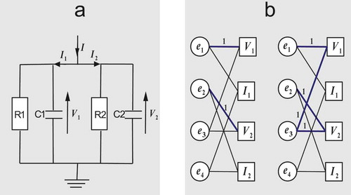
To simplify the illustration, the parameter values of capacitances, i.e. and
, and resistances, i.e.
and
, are fixed to the value one. The only parameter remaining is the input current
. The voltage and the current through an electrical circuit with
as a fixed input current is described through the following DAE
where s are equation labels. Additionally, its computational graphs before and after applying Algorithm 2 are shown in ). It can be shown that the electrical circuit DAE turns out to have a differential index of two.
4.1.1. Index reduction with the structural index
To accurately solve this system of equations using, say, a DAE solver, it needs to get transformed into a DAE of index one including the algebraic constraints. shows the computational graphs of the system of equations before and after one iteration of Algorithm 2. Using Definition 2.4 and denoting the computational graph , the structural index of the system of equations of the electrical circuit is computed as follows
By applying Algorithm 1 on the system of equations one obtains
The above system of equations is overdetermined if the algebraic constraint is included (i.e. five equations in four unknowns). By rather applying Algorithm 2, a consistent system of equations is constructed via the replacement of the time derivative
with an algebraic variable
Note that the new generated equation is not included in the underlying computational graph. The algorithm influences the computational graph only by incrementing the weight of edges incident to the selected equation. Now it can be shown that the structural index of the underlying computational graph is equal to one
The previous system of equations has structural index one and it can be solved via a DAE solver.
4.1.2. Structural index of sensitivity equation
Using Algorithm 3, the structural index of sensitivity equation
with can be reduced in a straightforward way as follows
It is easy to see that the AD-IR strategy results in the same system of equations as the IR-AD strategy. There is no need to apply Pantelides algorithm on the whole computational graph of the sensitivity equation.
4.2. The pendulum model example
) demonstrates the motion of a free pendulum in the Cartesian space (cf [Citation53]. Section 12.7.2). This is described by a second-order system of equations
Figure 2. The pendulum model and its computational graphs representation for two iterations of Algorithm 2.
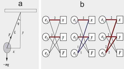
Additionally, its computational graphs after applying Algorithm 2 for two iterations are shown in ).
4.2.1. The structural index of the pendulum system of equations
It can be shown that the Pendulum system of equations is of differential index three (i.e. it requires three differentiation steps to get transformed into an explicit ODE system). The structural index can be shown to be equal to three as follows
4.2.2. Structural index of sensitivity equation
The sensitivity equation of the pendulum system of equations w.r.t. the parameters is as follows
where . The structural index of the sensitivity equation is reduced to one by applying Algorithm 3. Two iterations are performed in which equations
and
are differentiated two times. After one iteration, the sensitivity equation becomes
In the previous system of equations and
were replaced by
and
, respectively, according to the method of dummy derivatives. Alternatively, a dummy variable
and its derivatives
could have been introduced mainly satisfying line 5 in Algorithm 1 and line 9 in Algorithm 2. This will result in a rather different equation system, however, similarly leading to a reduced-index system after executing the main loop in Algorithm 3. After the second iteration, the sensitivity equation becomes as follows
Similarly, and
were replaced by
and
, respectively. The resulting system can be solved by a DAE solver if it is transformed into a first-order system (by introducing a dummy variable
).
5. Conclusion
In this work, a novel result concerning the structural index of sensitivity equation is presented. The relationship between the differential index of a DAE and that of the corresponding sensitivity equation is emphasized. It is concluded that both DAEs have an identical structural index. This implies that the differential index of both systems of equations is equal for a considerable class of systems, namely those DAEs with structural index identical to the differential index.
Due to the common structural characteristics of a DAE (1) and its corresponding sensitivity Equations (1) and (2), the index reduction process is computationally equal in terms of efforts in the context of sensitivity equation. As concluded by Theorem (3.2), if an equation is selected for differentiation towards structural index reduction, the corresponding equations
, obtained by differentiating
w.r.t.
, should be also chosen for index reduction of the whole sensitivity subsystem of Equation (2) (cf. Theorem 3.2 for the used notions).
As Definition 2.2 does not exclude DAEs of higher time derivatives, regardless of the fact that they can be rewritten as DAEs of order one, the conclusions made in this work are also applicable to DAEs of higher orders. This can be observed from the second-order system of equations in the presented example. The same statements also apply to sensitivity equation w.r.t. some model start values by which derivatives can be also present.
These theoretical results encourage the usage of the AD-IR strategy for performing sensitivity analysis of high-index differential algebraic equations. From one side, the IR-AD strategy is typically employed as the case with JModelica [Citation30]. The compiler capabilities of JModelica enhanced with AD techniques [Citation31] are exploited for linking generated index-reduced DAEs with highly specialized solvers within the SUNDIALS suite [Citation19]. The underlying state-of-the-art solver is based on a modern method for performing sensitivity analysis of DAEs. It exploits the structure of the sensitivity equation and the linearity of its extended Jacobian for efficient numerical integration. Moreover, specialized interfaces are provided for automatically differentiated routines (i.e. computer programs that have been automatically generated by AD tools, cf. www.autodiff.org) computing the required partial derivatives in Equation (2).
On the other side, the non-conventional AD-IR is an attractive choice for sensitivity analysis of high-level abstraction models. An example is given by the Modelica library ADGenKinetics [Citation32], which includes algorithmically differentiated components for modelling biochemical reaction networks. By simulating base models additionally embedding sensitivity equation, PSs are evaluated using arbitrary DAE solvers provided by the chosen Modelica simulation environment. From one side, direct numerical integration of large-scale systems becomes inefficient. From the other side, the advantages of employing modern DAE solvers for sensitivity analysis vanish with increasing nonlinearity of large-scale sensitivity systems [Citation55]. Nevertheless, an easily applicable modification of the parallelizable method from Dickinson and Gelinas [Citation56] can be used for retaining the efficiency of the AD-IR strategy. In this method, several smaller copies of sensitivity equation w.r.t. few parameters are simulated in parallel as shown in [Citation57] Section 16.3. Based on this work, similar tools and libraries based on the AD-IR strategy for AD of object-oriented models can be designed in future, for example the ADMSL library [Citation58].
A significant practical contribution of this work is to assess a potential enhancement to the Modelica language w.r.t. to the operator der, expressing time derivatives of state variables, e.g. der(x) . A way to express PS at Modelica language level is to allow a second parameter argument for the operator der to take place, i.e. der(x,p)
. This work shows that such an enhancement would not increase the compilation algorithmic complexity at least w.r.t. the process of index reduction. Another interesting point that needs to be investigated is whether the structure of sensitivity equations can be exploited to handle its robust initialization efficiently.
Acknowledgments
The first author acknowledges Austrian Institute of Technology as this article has been partially written during my employment there.
Disclosure statement
No potential conflict of interest was reported by the authors.
References
- H. Elmqvist and S.E. Mattsson, Modelica - The next generation modeling language: An international design effort, ESS97: The 9th European Simulation Symposium, October, Passau, Germany, 1997.
- P.J. Ashenden, G.D. Peterson, and D.A. Teegarden, The System Designers Guide to VHDL-AMS, Morgan Kaufmann, 2003.
- F.E. Cellier, Continuous System Modeling, Springer Verlag, 1991.
- H. Elmqvist, A structured model language for large continuous systems, Ph.D. thesis, Lund Institute of Technology, Lund, Sweden, 1978.
- S.E. Mattsson, Simulation of object-oriented continuous time models, Math Comput Simul 39 (1995), pp. 513–518.
- K.E. Brenan, S.L. Campbell, and L.R. Petzold, Numerical Solution of Initial-Value Problems in Differential-Algebraic Equations, North-Holland, New York, NY, 1989.
- F. Casella, F. Donida, and M. Lovera, Beyond simulation: Computer-aided control system design using equation-based object-oriented modelling for the next decade, Simul. News Europe 19 (2009), pp. 29–41.
- M. Günther and U. Feldmann, The DAE-index in electric circuit simulation, Math Comput Simul 39 (1995), pp. 573–582.
- P.C. Müller, Descriptor systems: Pro and cons of system modelling by differential-algebraic equations, Math Comput Simul 53 (2000), pp. 273–279.
- P. Schwarz, Simulation of systems with dynamically varying model structure, Math Comput Simul 79 (2008), pp. 850–863.
- C.W. Gear and L.R. Petzold, ODE methods for the solution of differential/algebraic systems, Siam J. Numer. Anal. 21 (1984), pp. 716–728.
- S.L. Campbell, A computational method for general higher index nonlinear singular systems of differential equations, IMACS Trans. Scientific Comput. 1 (1989), pp. 555–560.
- S.L. Campbell and E. Moore, Constraint preserving integrators for general nonlinear higher index daes, Numerische Mathematik 69 (1995), pp. 383–399.
- J.D. Pryce, Solving high-index DAEs by Taylor series, Numer. Algorithms 19 (1998), pp. 195–211.
- C. Tischendorf, Regularization of electrical circuits, IFAC-PapersOnLine 48 (2015), pp. 312–313. Available at. Available at http://www.sciencedirect.com/science/article/pii/S2405896315002177.
- C.C. Pantelides, The consistent initialization of differential-algebraic systems, SIAM J. Sci. Stat. Comput. 9 (1988), pp. 213–231.
- B. Bachmann, P. Aronsson, and P. Fritzson, Robust initialization of differential algebraic equations, Modelica’2006: The 5th International Modelica Conference, Vienna, Austria, 2006.
- S.E. Mattsson and G. Söderlind, Index reduction in differential-algebraic equations using dummy derivatives, SIAM J. Sci. Comput. 14 (1993), pp. 677–692.
- A.C. Hindmarsh, P.N. Brown, K.E. Grant, S.L. Lee, R. Serban, D.E. Shumaker, and C.S. Woodward, SUNDIALS: Suite of nonlinear and differential/algebraic equation solvers, ACM Trans. Math. Software, 31 (2005), pp. 363–396. Available at http://doi.acm.org/10.1145/1089014.1089020
- A. Griewank and A. Walther, Evaluating Derivatives: Principles and Techniques of Algorithmic Differentiation, 2nd ed., no. 105 in Other titles in Applied Mathematics, SIAM, Philadelphia, PA, 2008.
- U. Naumann, The Art of Differentiating Computer Programs, an Introduction to Algorithmic Differentiation, SIAM, 2012.
- W. Braun, L. Ochel, and B. Bachmann, Symbolically derived Jacobians using automatic differentiation - Enhancement of the openmodelica compiler, Modelica’2011: The 8th International Modelica Conference, March, Dresden, Germany, 2011.
- F. Casella, F. Donida, B. Bachmann, and P. Aronsson, Overdetermined steady-state initialization problems in object-oriented fluid system models, Modelica’2008: The 6th International Modelica Conference, March, Bielefeld, Germany, 2008.
- D.E. Schwarz and R. Lamour, A new approach for computing consistent initial values and Taylor coefficients for DAEs using projector-based constrained optimization, Numer. Algorithms 78 (2017), pp. 355–377.
- S. Li, L. Petzold, and W. Zhu, Sensitivity analysis of differential-algebraic equations: A comparison of methods on a special problem, Appl. Numer. Math. Trans. IMACS 32 (2000), pp. 161–174.
- M. Caracotsios and W.E. Stewart, Sensitivity analysis of initial value problems with mixed ODEs and algebraic equations, Comput. Chem. Eng. 9 (1985), pp. 359–365.
- R. Tomović and M. Vukobratovíc, General Sensitivity Theory, Modern Analytic and Computational Methods in Science and Mathematics, American Elsevier Pub. Co., 1972.
- A. Elsheikh, An equation-based algorithmic differentiation technique for differential algebraic equations, J. Comput. Appl. Math. 281 (2015), pp. 135–151.
- A. Elsheikh and W. Wiechert, Automatic sensitivity analysis of DAE-systems generated from equation-based modeling languages, in Advances in Automatic Differentiation, C.H. Bischof, H.M. Bücker, P.D. Hovland, U. Naumann, and J. Utke, eds., Springer, 2008, pp. 235–246.
- J. Åkesson, K.E. Årzén, M. Gäfvert, T. Bergdahl, and H. Tummescheit, Modeling and optimization with Optimica and JModelica.org–Languages and tools for solving large-scale dynamic optimization problem, Comput. Chem. Eng. 34 (2010), pp. 1737–1749.
- J. Andersson, J. Åkesson, F. Casella, and M. Diehl, Integration of CasADi and JModelica.org, Modelica’2011: The 8th International Modelica Conference, March, Dresden, Germany, 2011.
- A. Elsheikh, ADGenKinetics: An algorithmically differentiated library for biochemical networks modeling via simplified kinetics formats, Modelica’2012: The 9th International Modelica Conference No. 076 Linköping Electronic Conference Proceedings, September, Munich, Germany, 2012, pp. 915–926.
- W. Wiechert, S. Noack, and A. Elsheikh, Modeling languages for biochemical network simulation: Reaction vs equation based approaches, Adv. Biochem. Eng. Biotechnol. 121 (2010), pp. 109–138.
- A.K. Gupta and S.A. Forth, An AD-enabled optimization toolxbox in LabVIEWTM, in Recent Advances in Algorithmic Differentiation, S. Forth, P. Hovland, E. Phipps, J. Utke, and A. Walther, eds., Lecture Notes in Computational Science and Engineering, Vol. 87, Springer-Verlag Berlin Heidelberg, 2012, pp. 285–295.
- U.M. Ascher and L.R. Petzold, Computer Methods for Ordinary Differential Equations and Differential-Algebraic Equations, SIAM, 1998.
- E. Hairer and G. Wanner, Solving Ordinary Differential Equations II Stiff and Differential-Algebraic Problems, Vol. 14, Springer Series in Computational Mathematics, 2004.
- J.B. Keiper and C.W. Gear, The analysis of generalized backward difference formula methods applied to hessenberg for differential-algebraic equations, SIAM J. Numer. Anal. 28 (1990), pp. 833–858.
- P. Lötstedt and L. Petzold, Numerical solution of nonlinear differential equations with algebraic constraints. ii: Practical implications, SIAM J. Sci. Stat. Comput. 7 (1986), pp. 720–733.
- E. Hairer, C. Lubich, and M. Roche, The Numerical Solution of Differential-Algebraic Systems by Runge-Kutta Methods, Lecture Notes in Mathematics, Vol. 1409, Springer, 1989.
- A. Leitold and K.M. Hangos, Structural solvability analysis of dynamic process models, Comput. Chem. Eng. 25 (2001), pp. 1633–1646.
- E. Griepentrog and R. März, Differential-Algebraic Equations and Their Numerical Treatment, Teubner-Texte zur Mathematik [Teubner Texts in Mathematics], Teubner Verlagsgesellschaft, Leipzig, 1986.
- P. Kunkel and V. Mehrmann, Differential-Algebraic Equations: Analysis and Numerical Solution, EMS Textbooks in Mathematics, European Mathematical Society, 2006.
- W. Seiler, Indices and solvability for general systems of differential equations, CASC’99, the 2nd Workshop on Computer Algebra in Scientific Computing, Munich, Germany, 1999, pp. 365–385.
- S.L. Campbell and C.W. Gear, The index of general nonlinear DAEs, Numerische Mathematik 72 (1995), pp. 173–196.
- C.W. Gear, Differential algebraic equations, indices, and integral algebraic equations, SIAM J. Numer. Anal. 27 (1990), pp. 1527–1534.
- G. Reissig, W.S. Martinson, and P.I. Barton, Differential–Algebraic equations of index 1 may have an arbitrarily high structural index, SIAM J. Sci. Comput. 21 (1999), pp. 1987–1990.
- P. Bujakiewicz and P. van den Bosch, Determination of perturbation index of a DAE with maximum weighted matching algorithm, Proceeding of IEEE/IFAC Joint Symposium on Computer-Aided Control System Design, March, 1994, pp. 129–136.
- K. Murota, Systems Analysis by Graphs and Matroids, Springer, Berlin, 1987.
- J.A. Bondy, Graph Theory with Applications, Elsevier Science Ltd, Oxford, UK, 1976.
- J. Frenkel, G. Kunze, and P. Fritzson, Survey of appropriate matching algorithms for large scale systems of differential algebraic equations, Modelica’2012: The 9th International Modelica Conference, September, Munich, Germany, 2012.
- J.E. Hopcroft and R.M. Krap, An n5/2 algorithm for maximum matchings in bipartite graphs, Siam J. Comput. 2 (1973), pp. 225–231.
- T. Uno, A fast algorithm for enumerating bipartite perfect matchings, in ISAAC 2001: The 12th Annual International Symposium on Algorithms and Computation, LNCS 2223, Springer-Verlag, 2001, pp. 367–379.
- P. Fritzson, Principles of Object-Oriented Modeling and Simulation with Modelica, Wiley-IEEE Computer Society Press, 2003.
- R.J. Trudeau, Introduction to Graph Theory, Dover Publications, New York, 1993.
- S. Li and L. Petzold, Software and algorithms for sensitivity analysis of large-scale differential algebraic systems, J. Comput. Appl. Math. 125 (2000), pp. 131–145.
- R. Dickinson and R. Gelinas, Sensitivity analysis of ordinary differential equation systems - a direct method, J. Comput. Phys. 21 (1976), pp. 123–143.
- A. Elsheikh, Modelica-based computational tools for sensitivity analysis via automatic differentiation, Dissertation, RWTH Aachen university, Aachen, Germany, 2013. Available at http://darwin.bth.rwth-aachen.de/opus3/volltexte/2014/4767/.
- A. Elsheikh, Modeling parameter sensitivities using equation-based algorithmic differentiation techniques: The ADMSL, Electrical Analog library Modelica’2014: The 10th International Modelica Conference, March, Lund, Sweden, 2014.