Modelling health impacts of hepatitis – model selection and treatment plans

ABSTRACT

Hepatitis B and C are viruses causing liver infections and resulting in grave secondary diseases. While there are different treatments for chronic liver infections, the process of evolving chronic diseases is still not fully understood. This paper presents an economic-inspired model for the overall health of an infected organism. The health model is based on the results of a reaction diffusion model for describing the space-dependent dynamics of virus and T cells during a liver infection. The different treatments affect the parameters of the reaction diffusion model and influence therefore the well-being of the infected person during an infection. The health model is selected in a detailed process out of a class of possible models. The presented work provides a foundation for an optimal control problem for finding the best treatment strategy.

KEYWORDS:

• Reaction diffusion model
• treatment plans
• health modelling

1. Introduction

Hepatitis B and C are globally spread viruses causing liver infections and affecting billions of people. Apart from acute infection courses, both diseases can also chronify leading to a long-term negative impact on patients’ health. The mechanisms that differentiate acute and chronic courses are still largely unknown [1]. While there are several suitable treatments for treating hepatitis B, hepatitis C cannot always be completely cured. In order to reduce the harm inflicted by a hepatitis virus and to reduce negative drug side effects personalized treatment plans are desired. In addition to the necessary clinical studies to evaluate treatment strategies, mathematical modelling provides the possibility for in-silico development and testing of treatment plans. However, in order to obtain helpful results, suitable mathematical models are required.

Building a mathematical model is challenging: A good model summarizes all important phenomenological effects for its application using a compact and abstract mathematical representation. Suitable mathematical models provide a foundation for simulative studies that reduce the need for biological experiments. Apart from biological experiments being expensive and time-consuming, there are open ethical questions concerning studies of hepatitis in humans and animals. Consequently, mathematical models provide a cheaper, quicker and ethically unproblematic opportunity for investigations.

From a model-theoretic point of view, a mathematical model should fulfil basic mathematical properties such as the existence of solutions and the dependency on parameters in a way that the model’s properties can be interpreted in the application domain. In the case of modelling hepatitis, the proposed model should have solutions interpretable as chronic and healing infection courses.

While several models have been previously published, these models only take into account the total virus load in the liver and do not describe a space-dependent distribution of the virus. However, in parts of the liver with a higher amount of virus the probability for damage of the tissue leading to cirrhosis is higher [2]. Therefore, the spatial distribution of virus is highly relevant, indicating that reaction diffusion equations are to be preferred over ordinary differential equations for modelling. Based on the models describing the dynamics of the virus during a liver infection, previously published papers propose models for optimizing the doses of medication during a treatment, i.e., for modelling treatment plans. The objective functions in these cases depend on the medication doses and also describe the drug side effects. Most of these published treatment models do not take the damage caused by the immune response into account. This damage leads to inflammation and causes cirrhosis as described above.

In summary, this leads to two research questions regarding spatial modelling of hepatitis infections via partial differential equations and arguing the model properties with respect to destructive secondary effects of the immune response. Hence, this paper proposes a new model for describing the health of an infected person during a liver infection. The dynamics of virus and cells of the immune system, namely T cells, are modelled with a reaction diffusion system including an integral term. Based on this model, the health is modelled by an economics inspired approach. Both virus and T cells influence the health of the infected person. Using this new model, treatments with different doses and different drugs are compared. This provides a basis for the design of treatment plans using optimal control methods.

1.1. Review of literature

There are some approaches for modelling different treatments for hepatitis B and C in the literature. In [3], a model consisting of three ordinary differential equations for the amount of free virus, uninfected and infected liver cells is presented. Based on this model, the effect of interferon-$\alpha$ on the viral load is studied and compared with medical data. As a result, the main effect of interferon-$\alpha$ is to block the release of free virus from infected cells. The model presented in [3] is a standard model for hepatitis B and C.

A comparable model was studied in [4]. The authors analyse the viral dynamics of hepatitis B under the influence of lamivudine. The model has as well as in [3] three ordinary differential equations and only considers the infection of healthy liver cells by free virus and do not consider cell-to-cell transmission. As a result of the optimization, a therapy with lamivudine only leads to a lower level of free virus but not directly of infected cells. Therefore, the authors in [4] recommend a mixed therapy.

Based on the model in [3], in [5] an adaptive control strategy for interferon-$\alpha$ therapy during hepatitis C infection is presented. As a new mechanism, the effectiveness of interferon-$\alpha$ is limited. The objective of the therapy is the number of infected cells, which should decrease to a lower limit.

On a different scale but with a comparable approach, in [6] an epidemic model for analysing the influence of treatment and vaccination on the transmission in the population is presented. The objective functional contains the infected compartments linearly and the regulation mechanisms like treatment and vaccination in quadratic terms. A combination of vaccination and treatment of infected is the optimal way for controlling the spread of hepatitis B in this setting.

Two approaches for optimal control of treatments are presented in [7] and [8]. Based on a model of three ordinary differential equations, which is comparable to the model in [3], the authors in [8] study the influence of interferon-$\alpha$ and ribavirin on the infection course. The objective functional depends linearly on the number of infected liver cells and quadratic on the amount of interferon-$\alpha$ and ribavirin. As a result, a high and constant amount of both medications is recommended for a rather long time.

In contrast to the objective in [8], the objective functional in [7] depends quadratically on the virus and the amount of infected liver cells. The model consists of four differential equations, where the virus is divided into intracellular capsids and free virus. Again, the objective depends quadratically on the amount of medication, here pegylated interferon-$\alpha$ and lamivudine. The optimal therapy derived from this approach are high and constant doses of both medicaments.

1.2. Focus of this work

The recent approaches present either models on the scale of a whole liver or on the size of a population. In this paper, we focus on a smaller scale, which still abstracts from the cell scale of the liver structure but regards the spread of virus in a part of the liver. We extend the ideas from [9] for the reaction diffusion model of [10]. The reaction diffusion model in [10] does not only describe the total amount of virus in the liver, like the models in [3–5,8] do, but it shows a space-dependent spread of virus in parts of the liver. In [9], the harm of virus and the programmed cell death caused by T cells during a liver infection was analysed. The investigations in [9] start with an ordinary differential equation for modelling the dynamics of virus and T cells in the liver. The model is a simplification of the model in [10]. Based on the ordinary differential equation system, the health during different infection courses was analysed. Due to the large damage of the programmed cell death and the inflammation, in some scenarios, a chronic liver infection with a rather weak immune reaction can lead to a higher health than a very strong immune reaction in the active phase.

In this paper, we focus on the full reaction diffusion system from [10] and define a new functional describing the overall health of an infected person with an economic-inspired approach as a value between zero and one. Both virus and T cells affect the health. The underlying model for virus and T cells is presented in Section 2.1. Some important mathematical properties of the systems solutions are given. Besides, solutions are interpreted as chronic and healing infection courses. In Section 2.2 a model for the health, based on homoeostasis, is chosen from a variety of possible models. The presented and analysed models differ in the mechanisms describing the harm of virus and T cells on the organism.

In Section 3, the health during acute and chronic liver infections is compared. Different medical treatments and their impact are presented in Section 4. The paper closes with conclusions and an outlook to optimal control strategies of infection courses.

2. Modelling liver infections and their impact on the organism

In this paper, liver infections are regarded on a length scale between the cell scale and a scale on the size of a whole liver. On this medium length scale, single cells are not displayed and the cell structure inside the liver tissue is, except for one feature, not regarded. The one modelled feature, which is part of the structure of the hepatic lobules, are portal fields. Blood and immune cells enter a lobule through a portal field. This structure feature is preserved during the modelling process of abstracting from the cell structure.

In the model, all cells of the immune response are combined as (general) T cells. In Section 2.1, a reaction diffusion model for the interplay between virus and T cells is presented, compare [10–12]. The model reproduces the two main infection courses of a liver infection, healing infections and chronic infections [2]. Healing infection courses have an active phase of inflammation in the beginning. Afterwards the virus vanishes and the immune reaction fades out. During a chronic infection course, the virus persists in some regions of the liver and the immune reaction remains on a medium level. Both, virus and immune reaction harm the liver tissue. Oftentimes, people with a chronic liver infection survive for many years or even decades [2]. However, a chronic infection course is often followed by secondary diseases like cirrhosis or liver cancer [2],, due to the permanent damage of the tissue.

An infection course usually has different phases, compare [2]. After the infection with a hepatitis virus, the replication of the virus is high and the secondary immune reaction is still weak. Usually, an active phase follows. During this time, the virus replication is still high but the immune reaction and consequently the inflammation is high as well. The active phase is followed either by a healing process or by a chronic phase.

Both virus and T cells affect the liver and decrease the functionality of the liver. The negative impact of the virus and the T cells on the overall health of an organism is modelled in Section 2.2. Due to the unknown mechanisms of the impact of an infection on the health function, different modelling approaches are presented and compared. The aim of the paper is to decide well founded for a health model and use this for studying the influence of treatment on the health.

2.1. Interaction between virus and immune system

Modelling liver infections on a length scale between the cell scale and the scale of a whole liver requires a choice of a suitable domain. As the liver is a three-dimensional organ, a three-dimensional domain, regarded as a cut out of some parts of the liver, would be an intuitive choice. [13, p. 32, 37] includes pathological images of the spread of T cells during an acute and a chronic infection in two dimensions. These qualitative observations are used for model validation. Therefore, the dynamics of the infection are modelled on a two-dimensional slice out of a small part of the liver, $\mathrm{\Omega }\subset {\mathbb{R}}^2$. In light of the application, the two-dimensional slice can be seen as a projection of a three-dimensional domain on two dimensions. The behaviour of the system does not change using a three-dimensional domain but the visualization improves on two dimensions. With the same argument, the domain $\mathrm{\Omega }$ will be chosen as a two-dimensional rectangle for simulation purposes. This visualization fits again the pathological images from [13]. As $\mathrm{\Omega }$ is a slice out of the liver, the boundary $\mathrm{\partial }\mathrm{\Omega }$ does not have biological meaning. We regard the cut off $\mathrm{\Omega }$ as a random cut and state therefore that the amount of virus and immune cells does not change between places right inside and right outside of $\mathrm{\Omega }$. This results in a zero flux boundary condition on $\mathrm{\partial }\mathrm{\Omega }$.

The subset $\mathrm{\Theta }\subset \mathrm{\Omega }$ describes a portal field through which T cells as sum of all cells of the immune systems enter the regarded part $\mathrm{\Omega }$ of the liver.

The authors in [11] present and analyse the following reaction diffusion system for the interplay and spreading of the virus $u$ and the T cells $v$. The dynamics during a liver infection are described by

(1) $\begin{array}{cccc}{u}_{,t}& =ug(u)-\gamma uv+\alpha \mathrm{\Delta }u& \hspace{0.17em}& \mathrm{f}\mathrm{o}\mathrm{r}\mathbf{x}\in \mathrm{\Omega },t>0,\\ v_{,t}& =j[u]-\eta (1-u)v+\beta \mathrm{\Delta }v& \hspace{0.17em}& \mathrm{f}\mathrm{o}\mathrm{r}\mathbf{x}\in \mathrm{\Omega },t>0,\\ u(0,\mathbf{x})& =u_0(\mathbf{x}),v(0,\mathbf{x})=v_0(\mathbf{x})& \hspace{0.17em}& \mathrm{f}\mathrm{o}\mathrm{r}\mathbf{x}\in \mathrm{\Omega },\\ 0& =\mathrm{\nabla }u\cdot \mathbf{n}=\mathrm{\nabla }v\cdot \mathbf{n}& \hspace{0.17em}& \mathrm{f}\mathrm{o}\mathrm{r}\mathbf{x}\in \mathrm{\partial }\mathrm{\Omega },t>0.\end{array}$(1)

The dynamics of the virus $u$ include a growth term $ug(u)$ with the growth function

(2) $g(u)=(1-u)\frac{u-u_{\mathrm{m}\mathrm{i}\mathrm{n}}}{u+\kappa },$(2)

describing a logistic growth with an Allee effect for small population, see [14]. The virus is normalized to a maximal capacity of $1$. If the population $u$ is smaller than $u_{\mathrm{m}\mathrm{i}\mathrm{n}}$, the growth term becomes negative. This describes the Allee effect of a small vanishing population [14].

The second reaction term of the virus dynamics is a predator-prey-reaction describing a decrease of virus in dependency on the T cells by $-\gamma uv$. In this sense, the virus can be seen as a prey for the T cells, acting as predators. This comparison motivates the naming of the virus as $u$ and of the T cells as $v$ referring to the classical Lotka-Volterra model.

The third mechanism in the dynamics of the virus is a diffusive spreading of the virus. This mechanism abstracts from the different approaches of viral spread either by cell-to-cell transmission or via free virus, compare [4].

The dynamics of the T cells consist of three reaction terms and a diffusive spreading. The first reaction term $j[u]$ describes the inflow of T cells through the portal field $\mathrm{\Theta }$. The brackets highlight the fact that $j$ is a functional depending, for example, on the integral of $u$ over $\mathrm{\Omega }$. The increase of T cells depends on the total amount of virus in $\mathrm{\Omega }$. With a function ${\chi }_{\mathrm{\Theta }}(\mathbf{x})\ge 0$ on $\mathrm{\Theta }\subset \mathrm{\Omega }$ and ${\chi }_{\mathrm{\Theta }}(\mathbf{x})=0$ on $\mathrm{\Omega }\mathrm{\setminus }\mathrm{\Theta }$ fulfiling

(3) ${\int }_{\mathrm{\Theta }}{\chi }_{\mathrm{\Theta }}(\mathbf{x})\mathrm{d}\mathbf{x}=1,$(3)

the inflow is described by

(4) $j[u](\mathbf{x})=\delta {\chi }_{\mathrm{\Theta }}(\mathbf{x}){\int }_{\mathrm{\Omega }}u(t,\mathbf{x})\mathrm{d}\mathbf{x},$(4)

where $\delta \in {\mathbb{R}}_{+}$ is a parameter for the inflow strength.

The term $-\eta (1-u)v$ splits up into a decay term $-\eta v$ and a predator-prey growth term $\eta uv$ for the predator $v$. Combined, an interpretation for the term uses the maximal capacity of the virus $u$ as 1. The combined term is non-positive for all $u$ and $v$ and describes the decay of T cells in the absence of virus. In this interpretation, the T cells decay less if virus is present.

System (1) uses homogeneous Neumann boundary conditions or zero flux conditions. This description is a simplification and can be interpreted either as a model for the boundedness of different regions by impermeable tissue in the liver [2], or as a random choice of $\mathrm{\Omega }$ out of the liver with the assumption of a constant amount of immune cells or virus on either side of the boundary.

The starting point of the model is set as a time right after the incubation time, which is the time the specific immune reaction needs to evolve. For hepatitis B, the incubation time ranges between one and six month, [2, p.587]. Specific cytotoxic T cells for hepatitis C show up between 5 and 9 weeks after infection [2, p. 639]. In the model, the time $t=0$ marks the time at which the specific immune reaction starts reacting. Right after $t=0$, the immune reaction starts and $v$ is larger than zero. As the incubation time is rather long, the virus spreads out in the tissue for a long time and results in a realistic assumption of a large viral load. The initial conditions in (1) are a maximal virus concentration $u_0(\mathbf{x})\equiv 1$ and a zero T cell population $v_0(\mathbf{x})\equiv 0$. These initial conditions can be seen as natural initial conditions due to the incubation time of viral infections.

Remark 1. The natural initial conditions of system (1) are $u_0(\mathbf{x})\equiv 1$ and $v_0(\mathbf{x})\equiv 0$ for all $\mathbf{x}\in \mathrm{\Omega }$.

In [11], different initial conditions were studied as well and the systems behaviour does not change for initial conditions with small but positive $v_0$ and values $u_0$ smaller than 1 [15]. gives a proof for the global existence and boundedness of a solution of (1).

Remark 2. Solutions of (1) are non-negative and bounded for all time, i.e. $u(t,\cdot ),v(t,\cdot )\in L_{\mathrm{\infty }}(\mathrm{\Omega })$.

The solutions $u(t,\mathbf{x})$ and $v(t,\mathbf{x})$ of (1) are space and time dependent. Therefore, we define the $L_1(\mathrm{\Omega })$-norms of $u$ and $v$, which are due to the non-negativity of $u$ and $v$, see Remark 2, identical to the space integrals over $u$ and $v$.

Definition 2.1. The total amount of virus, respectively, T cells, in $\mathrm{\Omega }$ is given by the $L_1(\mathrm{\Omega })$-norms

(5) $\begin{array}{c}U(t)={\int }_{\mathrm{\Omega }}u(t,\mathbf{x})\mathrm{d}\mathbf{x}\mathrm{a}\mathrm{n}\mathrm{d}V(t)={\int }_{\mathrm{\Omega }}v(t,\mathbf{x})\mathrm{d}\mathbf{x}.\end{array}$(5)

Depending on the parameters, system (1) shows two characteristic solutions that are interpreted as healing and chronic infection courses. In the simulations, the domain $\mathrm{\Omega }$ is a two-dimensional square with length $1$. This domain is comparable to the pathological images in [13, p. 32, 37] showing the spread of T cells during an acute and a chronic infection. The portal field $\mathrm{\Theta }$ is modelled as a rectangular with the size of $0.14\times 0.14$ in the corner around $(x_1,x_2)=(1,1)$. With the homogeneous Neumann boundary conditions as a model for equal values inside and outside the boundary, the modelled domain can be regarded as a quarter of a larger cut out of the liver where the portal field is in the middle. The choice of this simulation domain allows a qualitative comparison between the simulation results and the pathological image.

In the simulations, the function ${\chi }_{\mathrm{\Theta }}(\mathbf{x})$ is the usual characteristic function, which has a fixed value $1/|\mathrm{\Theta }|$ for $\mathbf{x}\in \mathrm{\Theta }$ and zero for all $\mathbf{x}\in \mathrm{\Omega }\mathrm{\setminus }\mathrm{\Theta }$. The positive value $|\mathrm{\Theta }|$ gives the size of the domain $\mathrm{\Theta }$.

Example 2.2 (Healing infection courses). The solution of (1) with the parameters $u_{\mathrm{m}\mathrm{i}\mathrm{n}}=0.05$, $\kappa =0.01$, $\gamma =0.4$, $\alpha =0.6$, $\delta =1$, $\eta =0.2$, $\beta =3$ and the initial conditions $u_0(\mathbf{x})\equiv 1$ and $v_0(\mathbf{x})\equiv 0$, tends to zero. It fulfils

(6) $\underset{t\to \mathrm{\infty }}{lim}u(t,\mathbf{x})=\underset{t\to \mathrm{\infty }}{lim}v(t,\mathbf{x})=0$(6)

and is interpreted as a solution connected to a healing infection course.

Figure 1 shows the space-dependent solution for a fixed time $t$ and the phase diagram of the $L_1(\mathrm{\Omega })$-norms $U,V$.

Figure 1. Dynamics of a solution of system (1) interpreted as a healing infection course. (a) and (b) show the virus and T cell population at $t=1.5$. Around $(x_1,x_2)=(1,1)$, the T cell population is higher due to the inflow area $\mathrm{\Theta }$. Starting with initial conditions $u_0(\mathbf{x})\equiv 1$ and $v_0(\mathbf{x})\equiv 0$, the T cell population increases and the virus vanishes first. Afterwards, the T cells decrease to zero as well, compare the $L_1(\mathrm{\Omega })$-phase diagram in (c).

The space-dependent solution in Figure 1 shows the infection in an acute phase. This phase lasts weeks too few months for hepatitis B and C [2, p. 587, 640]. As the convergence to a close to zero value takes a time span of 30, a suitable time unit is month, so Figure 1(a,b) shows the spread after $t=1.5$ month. During the active phase, the amount of T cells may reach very large values [2, p. 614].

The spread of T cells in the whole domain $\mathrm{\Omega }$ is comparable to the pathological image in [13, p. 32] and the description in [2, p. 588] saying that the inflammation involves the whole liver. As $\mathrm{\Omega }$ is projection of a random part of the liver, the spreading over whole $\mathrm{\Omega }$ is comparable to a spread in the whole liver.

Example 2.3 (Chronic infection courses). The solution of (1) with the parameters $u_{\mathrm{m}\mathrm{i}\mathrm{n}}=0.05$, $\kappa =0.01$, $\gamma =0.4$, $\alpha =0.6$, $\delta =0.8$, $\eta =0.2$, $\beta =0.65$ and the initial conditions $u_0(\mathbf{x})\equiv 1$ and $v_0(\mathbf{x})\equiv 0$ tends to a spatially inhomogeneous stationary state. It is interpreted as a chronic infection course.

Figure 2 shows the space-dependent solution for a fixed time $t$ during the chronic phase of the infection in (a) and (b) and the phase diagram of the $L_1(\mathrm{\Omega })$-norms $U,V$ in (c).

Figure 2. Dynamics of a solution of system (1) interpreted as a chronic infection course. (a) and (b) show the virus and T cell population at $t=25.5$, which is a time during the stationary phase. Around $(x_1,x_2)=(1,1)$, the T cell population is higher due to the inflow area $\mathrm{\Theta }$. Starting with initial conditions $u_0(\mathbf{x})\equiv 1$ and $v_0(\mathbf{x})\equiv 0$, both populations tend in the phase diagram of the $L_1(\mathrm{\Omega })$-norms to a stationary distribution, compare (c).

A chronic infection course may have an acute phase like in the healing infection course but oftentimes there is no active phase with a strong immune reaction [2]. The chronic infection course lasts for month or even years. Therefore, the time unit is again month, just like in Figure 1.

The space-dependent solution shows a higher amount of T cells around the portal field $\mathrm{\Theta }$. This is in accordance with the pathological images in [13, p. 37] and the description therein. Additionally, the inflammation, caused by cytotoxic T cells, varies between different small parts of the liver.

The two types of solutions in Example 2.2 and 2.3 are used as reference configurations for testing the models of the health function in Section 3. Even if the examples give exact parameters, a wide range of parameters provide similar solutions, see [11]. The chosen parameter values are not adapted to real data but can be interpreted in light of application. The minimal value $u_{\mathrm{m}\mathrm{i}\mathrm{n}}$ is a value under which the virus vanishes. This can be interpreted as a local immune reaction. In both examples, this value remains constant, as well as the scaling parameter $\kappa$, which scales the virus reproduction, and the two other parameters influencing the virus dynamics. The parameter $\gamma =0.4$ is constant and describes the effectiveness of the cytotoxic T cells in attacking the virus or, on a smaller scale, the probability that a cytotoxic T cell recognizes an infected liver cell and causes the programmed cell death that kills the virus in the liver cell. The diffusion of the virus is scaled by $\alpha =0.6$, describing the spreading from parts with higher virus concentration to parts with lower concentration.

The two solution types are, in these examples, influenced by the parameters regulating the T cell dynamics. The parameter $\delta$ varies the inflow of T cells through the portal field. In Example 2.2, this value is higher than in Example 2.3. This means that the same viral load results in more T cells in the example with a healing infection course. Additionally, in the example with a healing infection course, the spreading parameter $\beta$ is larger. The third parameter $\eta$ influencing the T cells describes the reduction of T cells in absence of virus and is constant for the two examples.

Altogether, a higher amount of T cells and a higher agility of the T cells lead to a healing infection course instead of a chronic course.

2.2. Overall health of an infected organism

In [9], a model for the burden on the organism caused by a liver infection is presented. The model was developed for an ordinary differential equation system describing the dynamics of a liver infection. There, the variable $w$ describes the wealth or well-being of an infected person and is given as a solution of the differential equation

(7) $\dot{w}=z(1-\zeta u)-\mu v$(7)

with an initial condition $w(0)=w_0$, $z,\zeta ,\mu >0$. The burden $B$ of an organism during an infection is defined as

(8) $B={\int }_0^{\mathrm{\infty }}{\left[\frac{1}{4}(zt+w_0)-w(t)\right]}^{+}\mathrm{d}t,$(8)

which can be interpreted as the area between the curve of a quarter of the wealth of a healthy person and an infected person. Only the positive difference between the reference wealth and the wealth of an infected is integrated, see [9].

The model in (7) describes the reduced increase of the overall wealth of an organism and is based on an economic approach for describing the output of the metabolism. In this mindset, the organism increases its wealth in every time step with a higher metabolic output than necessary for surviving. Both the virus $u$ and the T cells $v$ decrease the wealth. While the influence of the virus $u$ reduces the increase of wealth as a result of the higher metabolic output, the T cells $v$ affect the wealth more directly.

In the present paper, we change the point of view from this economic approach of describing the increase of well-being over time to a description of the total health as a number between zero and one. The change of health describes the general impact of an infection on the body.

We regard a healthy organism without further restrictions to the health. Therefore, an organism that is not affected by a virus increases its health until it is fully healthy. This assumption is comparable to the increase in health due to a higher metabolic output than necessary in (7). The organism can be regarded as a system tending towards a perfect health, compare the homoeostasis of a living organism. The underlying processes of the homoeostasis are not part of this model.

If an organism is infected by a virus, for example a hepatitis virus, the functionality of the organisms and some organs, like the liver, are decreased. The health is not increasing towards one as fast as a healthy organism does or the health is even decreasing. If the immune system is active, the health is decreasing as well. Both virus and T cells harm the organism and decrease the health. In sense of the homoeostasis, the infection is an external influence on the balanced process.

The way of harming the organism differs between the virus and the cells of the immune system. The virus replicates in liver cells and therefore the liver function is decreased. T cells search for infected liver cells and trigger the programmed cell death of an infected liver cell. In this way, the virus inside the liver cell is killed together with the liver cell. The programmed cell death causes inflammation [2,16]. Therefore, the T cells harm the organism by causing inflammation.

Starting with the balancing process towards perfect health, we present different mechanisms for describing the influence of virus and T cells on the health. Combining the mechanisms creates a model family for describing the external influenced homoeostasis. This model family is analysed analytically and numerically.

The first mechanism describes the increase of the health for a healthy person. In the absence of any infection, even a reduced health increases until it is maximal, compare the economic approach. We describe this increase of health by a non-negative function $q(w)$ with $q(1)=0$. This property ensures that $w$ is bounded by $1$, which is interpreted as perfect health.

In the absence of an infection, the health $w$ is modelled by the equation

(9) $\dot{w}=q(w)$(9)

with an initial health $w(0)=w_0\in [0,1]$. This is the underlying homoeostasis of the organism. A simple and well-motivated choice for the growth function of the health is a logistic growth

(10) $q(w)=w(1-w),$(10)

which is non-negative for $w\in [0,1]$ and fulfils $q(1)=0$.

The first assumption for modelling the influence of virus and T cells on the health is that the total amount of virus and the total amount of T cells in $\mathrm{\Omega }$ influences the health, compare Def. 2.1. Figure 1(c) and Figure 2(c) show the total virus and T cell populations for different infection courses.

Two general functions are added in the dynamics for describing the influence of the total amount of virus $U$ and T cells $V$ on the health.

Definition 2.4. The dynamic of $w$ influenced by the total amount of virus $U$ and the total amount of T cells $V$ is described by

(11) $\dot{w}=q(w)+F(U,w)+G(V,w)\mathrm{f}\mathrm{o}\mathrm{r}t>0,w(0)=w_0,$(11)

where $q(w)$ is a non-negative growth function with $q(1)=0$, and $F,G$ are non-positive smooth functions depending on the health $w$ and the total virus $U$ or the total T cells $V$. The functions $F$ and $G$ fulfil $F(0,w)=0$, $G(0,w)=0$ and are monotonously decreasing in $U$ respectively $V$.

Now, we present different approaches for $F$ and $G$ with positive parameters $a_i,b_i\in \mathbb{R}$.

A simple approach for modelling the decrease of health caused by the virus or the T cells is linear functions

(12) $F_1(U,w)=F_1(U)=-a_{1}U,G_1(V,w)=G_1(V)=-b_{1}V,$(12)

depending only on the virus or on the T cells but not on the health itself. These mechanisms describe the direct impact of T cells or virus on the change of health. Larger values of $U$ and $V$ lead to a larger decrease of the increase of health, which may result in a decrease of health. There is no influence of the actual health on the impact of virus $U$ or T cells $V$ on the change of health $\dot{w}$.

The second type of mechanisms includes a dependency of the actual health on the impact of virus $U$ or T cells $V$ on the change of health $\dot{w}$. Here, the idea starts with describing the balancing tendency of health towards a perfect health, $w=1$. The presence of virus and T cells reduces the ability of balancing towards $1$. The functions $F$ and $G$ of this mechanism type are

(13) $F_2(U,w)=-a_{2}wU,G_2(V,w)=-b_{2}wV.$(13)

A model consisting of mechanisms with this type reads

$\dot{w}=w(1-w-a_{2}U-b_{2}V).$

A lower health $w$ reduces the ability of both, an increase of health due to the balancing process and a decrease of health due to a high number of virus $U$ or T cells $V$. This behaviour can be interpreted as a lower ability of adaptation.

From a different point of view, the tendency to increase the health and the fight against the virus can be regarded as a competition for resources like metabolic energy. Analogously, sharing the resource of energy between the immune reaction and the tendency to increase health results in a competition model. The increase of health in the balancing process requires energy as well as living with a high amount of virus or with the effects of the T cells. The competition on energy takes place between the actions ‘increasing health’, ‘living with virus’ and ‘repairing damaged tissue’. (13) shows the competition terms as known from models for population dynamics with competition. A further discussion of models using this mechanism follows in Section 3.

Related to this approach, the competition can be regarded as a competition for resources regulating the increase of health. The maximal capacity in (9) is decreased through a competition term between the health and the virus or the T cells, in formula

(14) $F_3(U,w)=-a_3{w}^{2}U,G_3(V,w)=-b_3{w}^{2}V.$(14)

A model using these mechanisms can be written as

$\dot{w}=w(1-w-a_{3}wU-b_{3}wV),$

where the competition can be found in the brackets acting on the increase of health.

All three presented mechanisms for $F$ and $G$ are polynomials of the form $F(U,w)=P(w)U$ resp. $G(V,w)=P(w)V$, where $P=P(w)$ are polynomials up to an order of two. Of course, there are many more complex functions possible instead of polynomials. We will see in Section 3 that already the quadratic influence of $P(w)$ does not show the expected behaviour. All mechanisms are linearly in $U$ resp. $V$. This is in accordance with the approach in [8].

Some analytical results are summarized for the models. Section 3 compares the dynamics of the models during healing and chronic infection courses.

Remark 3 (Existence). The total amount of T cells $V$ is bounded by $V_{\mathrm{u}\mathrm{p}}=\frac{1}{\gamma }\left(1+\eta +\frac{\gamma \delta }{\eta }\right)|\mathrm{\Omega }|$, see [15]. The expression $|\mathrm{\Omega }|$ gives the size of $\mathrm{\Omega }$, $|\mathrm{\Omega }|={\int }_{\mathrm{\Omega }}1\mathrm{d}a$. The virus concentration is bounded by $1$ and therefore, the total virus population is bounded by $U_{\mathrm{u}\mathrm{p}}=|\mathrm{\Omega }|$. Consequently, the reaction functions in (1) and (11) are bounded in the positive domain and the solutions $u$, $v$ and $w$ exists for all time.

For a proof of this existence result see [15].

Remark 4 (Non-negativity). Models using the mechanisms $F_1$ or $G_1$ do not preserve the non-negativity of the solutions $w(t)$ of (11). The solutions of models using these mechanisms may become negative. In contrast, the solutions of models using only mechanisms $F_2$, $F_3$, $G_2$ and $G_3$ stay positive for any $U$, $V$ and all time $t$.

Remark 5 (Tendency towards perfect health). For all models combining the presented mechanisms, the state of perfect health, $w=1$ is a stable stationary point of (11) if $U,V\to 0$, that means if both, the virus and the T cells vanish.

In the next section, models using the presented mechanisms are compared for solutions interpreted as a healing and as a chronic infection course. The remarks in this section and the model results provide the possibility to select suitable models for further investigations. We discuss the model selection process and determine appropriate models out of a class of feasible models.

The evaluation of suitable models takes the real-world application, hepatitis, into account. Before combining different mechanisms to full models, the mechanisms itself are discussed here in light of hepatitis infections. The presented mechanisms are decreasing in dependency on the total virus $U$ and the total T cell amount $V$. Stronger infection and stronger inflammation lead to a smaller increase or even decrease of health. While the linear mechanisms $F_1$ and $G_1$ are independent of the health itself, the mechanisms $F_2$, $G_2$, $F_3$ and $G_3$ depend on the health. Regarding the balancing process towards a perfect health, the presence of virus and T cells leads to a competition for resources like metabolic energy. Therefore, the processes of increasing health and living with the infection and inflammation compete for energy. Modelling the competition results in the presented mechanisms $F_2$ and $F_3$, respectively, $G_2$ and $G_3$.

From a different point of view, mechanisms are thinkable describing that a lower health leads to a stronger decrease of health caused by infection or inflammation. As described in Section 2.1, there are people suffering from chronic hepatitis for years or even decades [2]. During this time, the health is reduced but many people live with the disease. Therefore, the assumption of a lower health leading to a stronger decrease of health is not suitable in this context.

3. Comparison of different health models

By using these three mechanisms for the influence of the virus and the T cell, nine different models are built for the dynamics of the growth in dependency on the solutions of (1), see Table 1. In this section, we evaluate the nine models in Table 1 by analysing the health during a healing and a chronic infection course.

Table 1. Overview of the model family for describing the health of an infected organism.

	$G_1$	$G_2$	$G_3$
$F_1$	model 1	model 2	model 3
$F_3$	model 4	model 5	model 6
$F_3$	model 7	model 8	model 9

As a preliminary consideration, we compare the three mechanisms for modelling a decrease of the health by just one component.

3.1. Building a model family

Figure 3 shows the decrease of health by just the virus $U$ and just by the T cells $V$ for the healing infection course in Figure 1 and the chronic infection course in Figure 2.

Figure 3. Comparison of the mechanisms in (12), (13) and (14) for a healing (solid) and a chronic (dashed) infection course. (a) Mechanism $F_1$ with $a_1=0.5$ in grey and ${\tilde{a}}_1=0.2\cdot a_1=0.1$ in black. (b) Mechanism $F_2$ with $a_2=0.5$. (c) Mechanism $F_3$ with $a_3=0.5$. The health is lower in the active phase. In both cases, healing and chronic infection courses, the health increases after the active phase. For healing infection courses, $w$ tends to one. (d) Mechanism $G_1$ with $b_1=0.5$ in grey and ${\tilde{b}}_1=0.2\cdot b_1=0.1$ in black. (e) Mechanism $G_2$ with $b_2=0.5$. (f) Mechanism $G_3$ with $b_3=0.5$. In the case of $G_1$ with $b_1=0.5$, the health falls below zero. In all other cases, the health is lowest during the active phase. In comparison to (a), (b) and (c) the health during a chronic infection remains lower.

Figure 3(a,d) show the linear decrease of health by (12) in black with a decreased decay constant and in grey with the same decay constant as in the two competition mechanisms. As one feature, the health in the shown examples only becomes negative in Figure 3(d) for the non-decreased parameter, compare Remark 4.

In general, the positivity of the health depends on the parameter and the maximal amount $U$ resp. $V$. Due to Remark 3, $U$ is bounded by $U_{\mathrm{u}\mathrm{p}}=|\mathrm{\Omega }|$ and $V$ is bounded by $V_{\mathrm{u}\mathrm{p}}$.

In case of a dependency of the health just on the virus, the change of health $\dot{w}=w(1-w)-a_{1}U$ becomes only negative, if at least the logistic growth is smaller than a threshold, which is here $w(1-w)<0.1$ due to the chosen parameters. This is the case for $w>0.89$ and $w<0.11$, see Figure 4. Consequently, the health in 3(a) with ${\tilde{a}}_1=0.1$ cannot fall below $0.89$, compare Figure 3(a). A more general result follows in Lemma 3.1.

Figure 4. Logistic growth (solid) compared to a fixed value $a_1{U}_{\mathrm{u}\mathrm{p}}=0.1$ and to the maximal decay from the competition mechanism $F_2$ in (13).

Additionally, Figure 4 shows the interplay between the competition mechanism in (13) and the logistic growth. For $U=1$, the competition mechanism in (13) reduces to $-a_{2}w$. For a large health, the logistic growth is smaller than the negative competition. Therefore, the health decreases. Even if the virus population remains maximal, the health cannot decrease lower than $w=0.5$.

Lemma 3.1. Let $U$ be the $L^1(\mathrm{\Omega })$-norm of the solution $u$ of (1) on a domain $\mathrm{\Omega }$ with $|\mathrm{\Omega }|=1$. In the system

(15) $\dot{w}=w(1-w)-a_{1}U$(15)

with an initial value $w(0)=w_0>0$ and $0<a_1<1/4$, the health $w$ cannot decrease below a minimal value $w_{\mathrm{m}\mathrm{i}\mathrm{n}}>0$.

Proof. The total virus amount $U$ is bounded by $|\mathrm{\Omega }|$, see Remark 3. Due to the requirements in the Lemma, $|\mathrm{\Omega }|=1$ and therefore $U\le 1$. Consequently, $f(w,U)=w(1-w)-a_{1}U\ge w(1-w)-a_1=\tilde{f}(w)$. For $a_1<1/4$, $\tilde{f}(w)$ got two positive zeros $w_{01}<w_{02}$ and $0<\tilde{f}(w)\le f(w,U)$ for $w\in (w_{01},w_{02})$. If the initial value $w(0)$ is larger than $w_{\mathrm{m}\mathrm{i}\mathrm{n}}=w_{02}$, then the logistic growth is larger than the virus depending on decay, compare Figure 4. Consequently, for all solutions $w$ with $w(0)>w_{\mathrm{m}\mathrm{i}\mathrm{n}}$, the health does not decrease below the value $w_{\mathrm{m}\mathrm{i}\mathrm{n}}$.□

Remark 6. The boundedness of the health $w$ from below in (15) reflects the observation, that many people live years suffering from chronic liver infectionswith comparable small viral loads [2].

The maximal total T cell amount $V_{\mathrm{u}\mathrm{p}}$ is in both parameter sets much larger. Consequently, the decay of the health is much stronger and possible for all health values $w$, even for the linear mechanism. In the following, we use the linear mechanism just with the reduced parameters ${\tilde{a}}_1$ and ${\tilde{b}}_1$. This reduces the tendency to decrease below zero in a short-time interval.

In the next step, the decay mechanisms in dependency on $U$ and on $V$ are combined like in (11).

Figure 5 shows the nine combinations of decay mechanisms in Table 1. The chosen parameters are, as in Figure 3, all identical with a scaling factor for the linear mechanisms. This scaling factor was already used in Figure 3 such that the health remains positive. The scaling factor $k$ allows a comparison ${\tilde{a}}_1=k{a}_j$ between the parameter for the linear mechanisms and the parameter for the other mechanisms. It enlarges the time interval of a non-negative solution for models using the mechanisms $F_1$ or $G_1$.

Figure 5. Health during an acute (solid) and chronic (dashed) infection course, compared for all nine models in Table 1. In model 2 and 3, the health decreases below 0 for chronic infection courses. Model 5 shows the largest decrease with non-negative $w$. Further explanations in the text.

As already seen in the visualization of the linear mechanisms in Figure 3 for the corrected parameter, the decay of health is in model 1 rather small. Models 2 and 3 show the decay of health below zero, due to the influence of the linear mechanism in dependency of the total virus $U$ additional to the reduction of health from the competition mechanism of the T cells $V$. Lemma 3.1 gives a minimal health if we only consider the linear influence of the total virus $U$ on the health. Now, the combination of a competition mechanism for the T cells and a linear mechanism for the virus shows a decay of the health below $0$.

This is a result of the decay by the competition mechanism, which leads to a decay of $w$ below a lower value $w_{\mathrm{l}\mathrm{o}\mathrm{w}}$. Figure 4 shows, that the logistic growth falls below a fixed value for small values of $w$. Consequently, it is possible that the decay of health caused by the competition mechanism of $V$ leads to such a low value $w_{\mathrm{l}\mathrm{o}\mathrm{w}}$ that the linear mechanism in dependency of $U$ is negative as well. This effect is visible in Figure 5 for model 2 and 3 for chronic infection courses, where the total virus $U$ and the total T cells $V$ tend to a positive stationary state.

The outcomes of model 1, model 4 and model 7 are comparable. The health falls in all three models during the active phase of both, the healing and the chronic infection course. After the active phase, the health increases during the healing course towards 1. In the chronic infection course, the health tends towards a stationary value depending on the used model.

The dynamics of the health in models 5 and 8 is similar as well. In comparison to model 4 and 7, the health decreases to a lower value during the active phase and stays lower during the chronic infection course. This result of the stronger decrease of health caused by the competition mechanism in dependency on the T cells, compare Figure 3.

Again, model 6 and model 9 provide quite similar results for the health. Models using the same mechanism depending on $V$ but different competition mechanisms for the decay in dependency of $U$ provide in all three cases similar results. Consequently, the influence of the competition mechanism in dependency of the total virus $U$ is rather small.

3.2. Evaluation and model selection

The combination of different mechanisms for the decay in dependency on the total virus $U$ and the total T cells $V$ leads to nine different models describing the change of health during liver infections. After presenting the modelling results, we evaluate the models with respect to the mathematical and biological observations. Following, we choose one model as best reflecting model out of the hierarchical model family. By regarding some models of all thinkable models, we preselected the mechanisms already in Section 2.2.

From a mathematical point of view, Remark 4 states that only models using competition mechanisms preserve the non-negativity of the health $w$. A zero value for the health could be interpreted as risk of death, but in this setting, we prefer to stick with a non-negative health $w>0$.

Remark 7. As a consequence of the choice of the health as a non-negative value, the models 1, 2, 3, 4, 7 using linear mechanisms are rated as not suitable for the modelling purpose. Therefore, the models 1, 2, 3, 4 and 7 are rejected.

The difference between model 5 and 8 is as well as the difference between model 6 and 9 small for the chosen parameters. With the aim to choose a model using as simple mechanisms as possible, compare Occams razor [17], model 5 and model 6 are favoured over model 8 and model 9.

From the nine models proposed in Table 1, the models 5 and 6 are so far appropriate for modelling the health during a liver infection. In model 5, the health is lower during the active phase than in model 6. This reflects the influence of a strong immune reaction on the organism and therefore fits the biological observations better.

On the other hand, the longterm health during a chronic infection course is higher in model 6. In model 5, the longterm health is quite low during the chronic infection course. This contradicts the biological observation that many infected people live with a chronic infection for years.

Models 5 and 6 are both suitable and have individual advantages and disadvantages. As a further investigation, we study the influence of the parameters $a_i,b_i$ on the health. So far, the parameters were chosen equally and with a random value, allowing to concentrate on the effects of the different mechanisms. Having chosen two suitable models, the investigations go further into detail. The aim of this investigation is to decide for one model combining the decreased health during the active phase and a rather high health during the chronic phase of the infection.

The parameters $a_i$ and $b_i$ describe the influence of virus, respectively, T cells on the health. A higher value represents a strong (negative) influence on health while a lower value stands for a smaller influence on health. The parameter choice is led by the question which parameters adapt the model best to the described medical observations, compare Section 2.1.

Figure 6 shows the health in model 5 and 6 for different parameter choices. A large impact of the virus, which is a result of a larger value $b_i$, has a large impact on model 5. The health decreases during both infection courses to a very low value, see Figure 6 in the upper right and upper left corner. The change of parameters on the health in model 6 is rather low. Model 6 shows in all parameter sets a rather high minimal health value.

Remark 8. The different parameter sets in Figure 6 show, that the health remains moderately high in model 6. This is in contrast to the biological observation of a life risk during an active inflammation.

Figure 6. Health during an acute (solid) and chronic (dashed) infection course, compared for model 5 and 6 and different parameter choices. The parameter $a_2$ gives the strength of the influence of the total virus $U$ on the health, $b_i$ the influence of the total T cells $V$.

Model 5 with the parameters $a_2=0.7$ and $b_2=0.3$ in the middle of the upper row in Figure 6 shows a decrease of health during the active phases of both, the healing and the chronic infection course. The health tends towards 1 during the healing course and to a value $w_{\mathrm{s}\mathrm{t}\mathrm{a}\mathrm{t}}=1-a_2{U}^{\star }-b_2{V}^{\star }$ with the stationary points $(U^{\star },V^{\star })$ of Figure 2. Model 5 reflects the lower health in the active phase. In the chronic phase, the health is higher. The health remains positive, compare Remark 4.

As a consequence of Occams razzor, more simple models are preferred over more complicated ones if both models provide the same information. Therefore, model 5 is preferred over model 6, which uses quadratic polynomials in $w$.

This section includes the comparison of the single mechanisms in the differential equation for the health. All nine combined models were tested for healing and chronic infection courses. After a further parameter choice for two models, which were chosen as the best of all nine models, a single model according to the biological observations was selected. The process of model selection shows the variability in modelling and highlights that the model was chosen in accordance with the observations and the principle of the simplest possible explanation. This provides an argument for only regarding the first polynomials $P(w)$ and not polynomials of order three and higher or different functions.

Concluding the evaluation of the nine models, we choose for further investigations model 5 with the parameters $a_2=0.7$, $b_2=0.3$, namely

(16) $\dot{w}=w(1-1)-0.7wU-0.3wV.$(16)

The results of this model are in common with most of the biological observations.

In the light of application, the parameter value $a_2=0.7$ reflects in comparison to $b_2=0.3$ a stronger influence of the viral load on health than the influence of the immune reaction on health. Remembering the fact that several infected people live with chronic infections and low immune response for many years, this parameter choice is questionable. On the other hand, the model quantities are a scaled virus amount and a non-scaled amount of T cells. Consequently, the amount of T cells $V$ may reach much larger values than the viral amount $U$, which is scaled to $|\mathrm{\Omega }|$. Therefore, a larger parameter $a_2$ in combination with a scaled $U$ does not lead automatically to a larger influence of the viral load on health compared to the immune reaction. The detailed study of different parameter sets in Figure 6 allowed a comparison with the medical observations.

4. Impact of treatment

Using the selected model with the mentioned parameters, we now analyse different medical treatments. After presenting current and older treatments, we compare different doses of medication. Therefore, some general conclusions about treatment and doses are given in Section 4.1.

There are various treatments for different hepatitis infections. First treatments of hepatitis C used interferon-$\alpha$, which activates the immune system and leads to a higher amount of T cells [5,18]. Starting in 1998 [18], a modified interferon-$\alpha$, called pegylated interferon-$\alpha$ was combined with ribavirin [5]. Additional to the effect on the immune system, ribavirin reduced the reproduction of the virus [18]. An important and significant improvement in the therapy of chronic hepatitis C infection was the development of direct acting antivirals (DAA). Instead of boosting the immune reaction, the DAA decreases the virus and its reproduction [18]. The amount of DAA and the frequency of doses depends on the specific type of hepatitis C virus. Therefore, every single patient needs an individual therapy. Additionally, the resistance of certain virus types on DAA increases [18].

For chronic hepatitis B infections, the common treatments still use interferon-$\alpha$ and pegylated interferon-$\alpha$. Using pegylated interferon-$\alpha$ reduces the frequency of doses from three doses per week to one dose per week. The combination of pegylated interferon-$\alpha$ with lamivudin, which reduces the replication of virus, is even more effective [7].

In all cases, the treatment and the dose of the medication depend, among others, on the viral load and on the inflammation values.

We classify three treatments according to the three mentioned therapy approaches. The first treatment reflects the treatment only with interferon-$\alpha$, which mainly influences the activity of the immune system.

Treatment 1. The interferon-$\alpha$ therapy affects only the T cells inflow, modelled in (1) by enlarging the inflow parameter $\delta$ in $j[u]$.

The combined treatment of pegylated interferon-$\alpha$ and ribavirin in the case of hepatitis C or pegylated interferon-$\alpha$ with lamivudin in the case of hepatitis B is the second treatment.

Treatment 2. The combined therapy of modified interferon-$\alpha$ in combination with an inhibitor like ribavirin or lamivudin, affects both, the T cells and the virus. In (1), the treatment 2 enlarges the T cell inflow via $\delta$ and decreases the replication of virus by reducing the growth of the virus. For modelling this influence, we add another parameter for the growth of the virus in (2) by setting $\tilde{g}(u)=\vartheta g(u)$. Without any treatment, the parameter $\vartheta$ is equal to 1. During treatment 2, the parameter $\vartheta$ is smaller than 1.

The third treatment is only available for hepatitis C infections. The direct acting antivirals reduce the replication of the virus much more effective than treatment 2 does.

Treatment 3. The direct acting antivirals reduce the reproduction of the virus significantly. In the setting of (1), this therapy results in a significant reduction of the new parameter $\vartheta$ scaling the growth and the maximal capacity of the virus.

Before testing the three treatments for chronic infection courses, we introduce an example showing the influence of medication in a simplified setting.

4.1. Influence of treatment on exponential growth

In simple models, there is an interesting influence of a treatment on the total growth observable. This example is also remarkable in competition models for the development of resistances, see [19].

Regard a model for a virus with an exponential, unbounded growth and without spatial distribution. The system

$u^{\mathrm{\prime }}=u\mathrm{w}\mathrm{i}\mathrm{t}\mathrm{h}u(0)=u_0$

has the solution $u(t)=u_0{\mathrm{e}}^t$. Now, a mechanism $\vartheta (t)$ with $\vartheta :[0,\mathrm{\infty })\to [0,1]$ is introduced, which regulates the exponential growth of $u$, so

(17) ${\tilde{u}}^{\mathrm{\prime }}=\vartheta (t)\tilde{u}\mathrm{w}\mathrm{i}\mathrm{t}\mathrm{h}\tilde{u}(0)=u_0.$(17)

The mechanism $\vartheta (t)$ can be written as well as $\vartheta (t)=1-\mathrm{\Theta }(t)$, where $\mathrm{\Theta }(t)$ models only the reduction.

The system in (17) has the solution

$\tilde{u}(t)=u_0{\mathrm{e}}^t{\mathrm{e}}^{-{\int }_0^t\mathrm{\Theta }(\tau )\mathrm{d}\tau }.$

The solution $\tilde{u}(t)$ depends on the influence $\mathrm{\Theta }(t)$, especially if $\mathrm{\Theta }(t)$ is not constant. If $\mathrm{\Theta }(t)$ models the influence of medication, $\mathrm{\Theta }$ is positive during the treatment and zero before and after the treatment. So, after a medication timespan $[0,T_{\mathrm{f}\mathrm{i}\mathrm{n}}]$, $\mathrm{\Theta }(t)$ is zero. Consequently, the reduction of growth does not depend on the exact treatment plan of $\mathrm{\Theta }(t)$ but on the total reduction ${\int }_0^{T_{\mathrm{f}\mathrm{i}\mathrm{n}}}\mathrm{\Theta }(\tau )\mathrm{d}\tau$ in the medication time interval.

By changing the variable $\tilde{u}$ to $z(t)=u(t){\mathrm{e}}^{-t}$, we find solutions $z$ being constant for $\mathrm{\Theta }=0$. The solution of (17) transforms into

$z(t)=u_0{\mathrm{e}}^{{\int }_0^t\mathrm{\Theta }(\tau )\mathrm{d}\tau ,}$

where the integral term describes the influence of any treatment $\mathrm{\Theta }(t)$. Any treatment $\mathrm{\Theta }$ leads to a change of the solution $z$, which can be regarded as percentile curves of $u$.

Figure 7 shows two different treatments $\mathrm{\Theta }$ in (a), which have the same integral term

(18) $d_{\mathrm{t}\mathrm{o}\mathrm{t}\mathrm{a}\mathrm{l}}={\int }_0^{T_{\mathrm{f}\mathrm{i}\mathrm{n}}}\mathrm{\Theta }(t)\mathrm{d}t.$(18)

Figure 7. Influence of treatment on the virus in (17). Solid lines belongs to one medication, dashed lines to two medication. (a) Doses of medication $\mathrm{\Theta }(t)$. (b) Solution $u(t)$, the dotted line shows the solution without treatment. (c) Transformed solution $z(t)$, the dotted line shows percentiles.

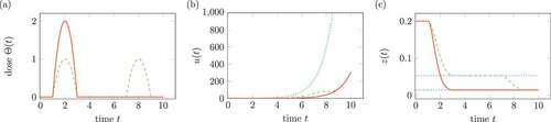
The integral $d_{\mathrm{t}\mathrm{o}\mathrm{t}\mathrm{a}\mathrm{l}}$ is interpreted as total dose of the medication. Figure 7(b) shows the comparison of solution $u(t)$ without medication and $\tilde{u}(t)$ for two different medications. In Figure 7(c), the percentiles of the transform $z$ are shown for both medications.

Regarding a logistic growth of virus instead of unbounded exponential growth, the solution depends on the time-dependent medication $\mathrm{\Theta }(t)$. Figure 8 shows the according results for the ordinary differential equation

(19) $u^{prime}=\vartheta (t)(1-u)u=(1-\mathrm{\Theta }(t))(1-u)u\mathrm{w}\mathrm{i}\mathrm{t}\mathrm{h}u(0)=u_0.$(19)

Figure 8. Influence of treatment on the system in (19). Solid lines belongs to one medication, dashed lines to two medication. (a) Doses of medication $\mathrm{\Theta }(t)$. (b) Solution $u(t)$, the dotted line shows the solution without treatment. (c) Transformed solution $z(t)$, the dotted line shows percentiles.

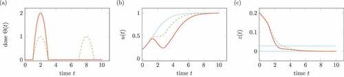
In contrast to Figure 7, the two medications do not lead to the same growth after medication. Consequently, we cannot expect that the mentioned treatments for the model in (1) are independent of the exact medication plan.

Remark 9. This result for the simplest growth model is surprising and does not reflect all medical treatment plans. In the following, we will test whether similar observations are possible for the model of T cells and virus in (1) and the treatments 1, 2 and 3.

In the following, the influence of the three introduced treatments on the virus and the T cells is studied. According to the type of treatment, the medication effects either the inflow of T cells, the reproduction of virus or both. The regulation of virus replication is an extension of the ideas of this section.

Influencing the virus reproduction or the inflow of T cells effects the health by the dynamics in (16). In this paper, a direct influence of medication on the health is not described. This limitation is addressed in Section ?

4.2. Testing treatment 1

For testing the influence of the hypothetical treatment 1, based on a pure interferon-$\alpha$ therapy, we regard the parameter set for chronic hepatitis infection from Ex. 2.3. The first assumption is that the treatment 1 changes the constant parameter $\delta$ into a time-dependent parameter $\delta =\delta (t)={\delta }_0+\tilde{\delta }(t)$, where ${\delta }_0$ is the constant parameter from Ex. 2.3 and $\tilde{\delta }(t)\ge 0$ for all time $t$ is the influence of interferon-$\alpha$.

We use a simple approach for modelling the influence of the medication on $\delta$. The time of medication be $t_{\mathrm{m}\mathrm{e}\mathrm{d}}$. For a time span of $t=2$, the value $\tilde{t}$ is larger than zero, in the sense, that

$\tilde{\delta }(t)=\left(\begin{array}{cc}d\cdot {(t-(t_{\mathrm{m}\mathrm{e}\mathrm{d}}+1))}^2,& \mathrm{f}\mathrm{o}\mathrm{r}{t}_{\mathrm{m}\mathrm{e}\mathrm{d}}<t<t_{\mathrm{m}\mathrm{e}\mathrm{d}}+2,\\ 0,& \mathrm{e}\mathrm{l}\mathrm{s}\mathrm{e}.\end{array}\right.$

Now, we vary between three medication plans. First, as treatment T1a, we only use one medication at time $t_{\mathrm{m}\mathrm{e}\mathrm{d}}$ with a dose $d$. Secondly, the treatment T1b consists of the doses with $\frac{d}{3}$ at times $t_{\mathrm{m}\mathrm{e}\mathrm{d}1},t_{\mathrm{m}\mathrm{e}\mathrm{d}2}$ and $t_{\mathrm{m}\mathrm{e}\mathrm{d}3}$, where $t_{\mathrm{m}\mathrm{e}\mathrm{d},i}-t_{\mathrm{m}\mathrm{e}\mathrm{d},j}=3$ for $i>j$, $i,j\in \{1,2,3\}$. As treatment T1c, we regard the effect of three medication times each with a dose $d$.

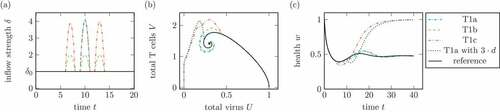
Figure 9(a) shows the time-dependent medications for treatment 1.

Figure 9. (a) Medication plan during treatment 1. T1a: One dose with $d$ at $t_{\mathrm{m}\mathrm{e}\mathrm{d}}=9$. T1b: Three doses with $d/3$ at $t_{\mathrm{m}\mathrm{e}\mathrm{d}1}=6,t_{\mathrm{m}\mathrm{e}\mathrm{d}2}=9$ and $t_{\mathrm{m}\mathrm{e}\mathrm{d}3}=12$. T1c: Three doses with $d$ at $t_{\mathrm{m}\mathrm{e}\mathrm{d}1}=6,t_{\mathrm{m}\mathrm{e}\mathrm{d}2}=9$ and $t_{\mathrm{m}\mathrm{e}\mathrm{d}3}=12$. (b) Phase plot of summed virus $U$ and summed T cells $V$ and (c) health during different treatments 1 and a reference infection course (solid). For comparison, T1a with $3\cdot d$ shows a single medication at $t_{\mathrm{m}\mathrm{e}\mathrm{d}}=9$ with a dose $\tilde{d}=3$. The treatments T1c and T1a with $3d$ show the transfer from a chronic to a healing infection course.

The model for medication is simple by using a polynomial of second order. It reflects that the body reacts not immediately on the medication and that the decay is not instantaneous, too.

Figure 9(b,c) show the dynamics of the total virus and the total T cells during the treatments in Figure 9(a). Only the treatments with a total dose of $4$, compare (18), namely treatment T1c and T1a with $3\cdot d$ lead to a healing infection course. The other treatments with a total dose of $\frac{4}{3}$ do not change the qualitative behaviour of the infection.

This example shows that the system (1) with treatment 1 inherits the simple property of (17) of the total dose being more important than the division into different doses.

Figure 9 shows that a treatment with a higher total dose leads to a lower health. All treatments start at around the time $t=10$, where the total health is around its minimum during the reference infection course without any treatment. Compared to the reference health, all treatments decrease the health for some time during the treatment. Nonetheless, every treatment leads to an increase in health during a time after the treatment, even if the treatments with a low total dose do not improve the health for a long time.

4.3. Testing treatment 2

The treatment 2 is comparable to the medication with pegylated interferon-$\alpha$ and ribavirin or lamivudin. This treatment effects both, the inflow of T cells via $\delta$ and the replication of the virus.

For modelling the influence on the virus replication, we specify the growth function in (2) by introducing a new parameter $\vartheta$. This parameter is in accordance with the growth reduction in (17). The growth of the virus is

(20) $ug(u)=\vartheta u(1-u)\frac{u-u_{\mathrm{m}\mathrm{i}\mathrm{n}}}{u+\kappa },$(20)

where the parameter $\vartheta$ is equal to 1 in the case of normal replication.

Analogously to treatment 1, we regard the effect of the medication during short-time intervals. In treatment 2, the virus replication parameter $\vartheta$ is reduced to a fixed value for the same time interval in which the inflow parameter $\delta$ in enlarged like in Figure 9(a).

Figures 10 and 11 show the virus and T cell dynamics and the health during different medication plans for treatment 2. The treatments T2a, T2b and T2c are defined according to the treatments T1a, T1b and T1c.

Figure 10. Comparison of different doses in treatment 2. (a) Phase plot of summed virus $U$ and summed T cells $V$ and (b) health during different treatments 2 and a reference infection course (solid). T2a is a one time treatment at time $t_{\mathrm{m}\mathrm{e}\mathrm{d}}=9$ with a dose $d=1$ and $\vartheta$ as given. T2b divides the dose $d$ into three doses with $\tilde{d}=1/3$ at three times $t_{\mathrm{m}\mathrm{e}\mathrm{d}}\in \{6,9,12\}$. T2c is a treatment with three doses $d=1$ at times $t_{\mathrm{m}\mathrm{e}\mathrm{d}}\in \{6,9,12\}$ and $\vartheta =0.8$.

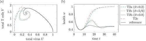
In Figure 10, two treatments lead to a healing infection course. On the one hand, T2a with a very low $\vartheta =0.2$ and maximal doses of $d=1$ leads to a healing course. In contrast, a higher replication factor $\vartheta$, for example $\vartheta =0.5$, leads to a chronic course. Secondly, treatments T2c with three high doses of medication leads to a healing course as well. The replication factor $\vartheta$ is comparable high with $\vartheta =0.8$.

The treatment T2c is the only shown treatment, where the health falls below the minimal health in the reference system. This is a consequence of not taken into account the side effects of medication.

As already seen in treatment 1, three doses of medication lead to a healing course independent of a reduced replication factor $a$.

Figure 11. Effect of the medication time. (a) Phase plot of summed virus $U$ and summed T cells $V$ and (b) health during two treatments 2 and a reference infection course (solid). The medication doses and parameters are identical in both medications, only the medication times change. The treatment with $t_{\mathrm{m}\mathrm{e}\mathrm{d}}\in \{6,9,12\}$ leads to a healing infections course, whereas the infection with medication times $t_{\mathrm{m}\mathrm{e}\mathrm{d}}\in \{16,19,22\}$ remains chronic.

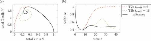
Figure 11 highlights the importance of the medication time. Both treatments use the same parameters, only the medication time changes. Whereas an early medication around $t=10$ leads to a healing infection course, the later medication does not affect the longtime infection course.

By reflecting treatment 2 as an interpretation of therapies using pegylated interferon-$\alpha$ and ribavirin or lamivudin, a very low replication factor $a$ seems unrealistic. A strongly reduced replication factor is more natural for direct acting antivirals, which are used in treatment 3.

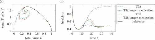
4.4. Testing treatment 3

Treatment 3 effects, according to the direct acting antivirals medicaments, only the reproduction of virus $\vartheta$. Remember, this treatment is only available for hepatitis C infections. For testing this treatment, we reduce the replication factor $\vartheta$ for some times. This effect was studied in a simplified setting in Section 4.1. Now, we regard the full system for virus, T cells and their influence on health.

Figure 12. Comparison of different treatments 3. (a) Phase plot of summed virus $U$ and summed T cells $V$ and (b) health during three treatments 3 and a reference infection course (solid). The treatment T3a uses $\vartheta =0.2$ and $t_{\mathrm{m}\mathrm{e}\mathrm{d}}=9$. For T3b, the parameter is reduced to a third of the effectiveness, $\vartheta =11/15$, and $t_{\mathrm{m}\mathrm{e}\mathrm{d}}\in \{6,9,12\}$. Treatment T3c with $\vartheta =0.5$ and $t_{\mathrm{m}\mathrm{e}\mathrm{d}}\in \{6,9,12\}$ leads to a healing infection course.

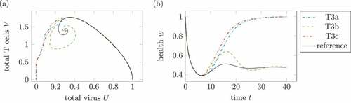
Figure 12 shows treatments according to the three mentioned treatment plans. The treatment T3a with only one dose reducing the reproduction rate $\vartheta$ to $\vartheta =0.2$ shows a healing infection course. In treatment T3b, the effective reduction is split up on three doses with $\vartheta =\frac{11}{15}$. The infection course remains chronic. Treatment T3c as a treatment with three high medication resulting in $\vartheta =0.5$ leads to a healing infection course. Of course, three doses with $\vartheta =0.2$ lead to healing infection courses, too.

Again, the infection course with treatment does not only depend on the total dose of medication but as well on the treatment plan itself.

Figure 13. Effect of longer medication times. (a) Phase plot of summed virus $U$ and summed T cells $V$ and (b) health during two treatments T3a and T3b and a reference infection course (solid). The maximal medication doses and parameters are identical in both medications, only the medication times change. In the longer treatments, the (third) treatments last double the time the other treatments does. The parameters are $\vartheta =0.5$ for T3a and $\vartheta =11/15$ for T3b. In the one dose treatment T3a, the longer medication time leads to a healing infection course.

Figure 13 compares two treatments of T3a and of T3b with different medication durations with each other. The treatment T3a uses $\vartheta =0.5$, which results for the standard medication duration $9<t<11$ in a chronic infection. By extending the medication time to $9<t<13$, the same maximal medication leads to a healing infection. The same method does not result in a healing infection course for treatment T3b with $\vartheta =\frac{11}{15}$.

In all three treatments, the health of infection courses which remains chronic show similarities. The medication leads to an increase of health during the treatment but after the medication fades out, the health sinks below the reference health of a chronic infection without treatment.

5. Conclusions and outlook to optimal control

Starting with a space-dependent model for the dynamics of virus and T cells during a liver infection, different mechanisms for modelling the influence of virus and T cells on the health of a healthy organism were presented. The mechanisms were linearly depending on the total virus or T cells amount in the regarded part of the liver. The different mechanisms were combined to nine different models. All models were tested with the numerical data of one chronic and one healing infection course. Based on the biological observations, two best fitting models for the health were chosen. By testing different parameter sets, one model was selected as the best describing model under the presented models for health.

This model was used for studying different treatments, which were connected to treatments with interferon-$\alpha$, lamivudine and directly acting antivirals. The medications had influence on the reaction diffusion model for the virus and T cells. For all three medications, different treatment plans with different doses were tested. In contrast to the simplest model for growth, the exact treatment was important and not only the total dose of medication.

The presented model for health is a good starting point for optimal control investigations. So far, the model does not contain a decrease of health due to side effects of medication. Therefore, the model provides first insights in the effectiveness of different treatments.

As a further investigations, costs for side effects of the medication can be added to the model for the health. In this case, a medication effects directly health by regarding side effects and indirectly via the change of virus and T cells

Besides, the reaction diffusion model for the dynamics of virus and T cells and the model for health can be treated under the aspects of optimal control. The main task is to find the best medication strategy and to compare the best strategies for all the medications.

Acknowledgement

We acknowledge support by the Open Access Publication Funds of Technische Universität Braunschweig.

Disclosure statement

No potential conflict of interest was reported by the author.

References

- E. Thomas and T.J. Liang, Experimental models of hepatitis B and C - New insights and progress, Nat Rev Gastroenterol. Hepatol. 136 (2016), pp. 362–374. doi:10.1038/nrgastro.2016.37
- E.R. Schiff, W.C. Maddrey, and M.K. Rajender, Schiff’s Diseases of the Liver, 12th ed., Wiley-Blackwell, Oxford, GB, 2018.
- A.U. Neumann, N.P. Lam, H. Dahari, D.R. Gretch, T.E. Wiley, T.J. Layden, and A.S. Perelson, Perelson Hepatitis C viral dynamics in vivo and the antiviral efficacy of interferon-αtherapy, Science. 2825386 (1998), pp. 103–107. doi:10.1126/science.282.5386.103
- M.A. Nowak, S. Bonhoeffer, A.M. Hill, R. Boehme, H.C. Thomas, and H. McDade, Viral dynamics in hepatitis B virus infection, PNAS. 939 (1996), pp. 4398–4402. doi:10.1073/pnas.93.9.4398
- S. Zeinali and M. Shahrokhi, Adaptive control strategy for treatment of hepatitis C infection, Ing. Eng. Chem. Res. 58 (2019), pp. 15262–15270. doi:10.1021/acs.iecr.9b02988
- A.V. Kamyad, R. Akbari, A.A. Heydari, and A. Heydary, Mathematical modeling of transmission dynamics and optimal control of vaccination and treatment for hepatitis B virus, Comput. Math Methods Med. 2014 (2014), pp. 475451. doi:10.1155/2014/475451
- K. Manna and S.P. Chakrabarty, Combination therapy of pegylated interferon and lamivudin and optimal controls for chronic hepatitis B infection, Int. J. Dynam. Control. 6 (2017), pp. 354–368. doi:10.1007/s40435-017-0306-x
- A. Mojaver and H. Kheiri, Dynamical analysis of a class of hepatitis C virus infection models with application of optimal control, Int. J. Biomath. 93 (2016), pp. 1650038. doi:10.1142/S1793524516500388
- C. Reisch and D. Langemann, Modeling the chronification tendency of liver infections as evolutionary advantage, Bull. Math. Biol. 81 (2019), pp. 4743–4760. doi:10.1007/s11538-019-00596-y
- H.-J. Kerl, D. Langemann, and A. Vollrath, Reaction-diffusion equations and the chronification of liver infections, Math Comput. Simulat. 82 (2012), pp. 2145–2156. doi:10.1016/j.matcom.2012.04.011
- C. Reisch, Reaktions-Diffusions-Gleichungen und Modellfamilien zur Analyse von Entzündungsprozessen, Dissertation, TU Braunschweig, Cuvillier, 2020.
- C. Reisch and D. Langemann, Chemotactic effects in reaction-diffusion equations for inflammation, J. Biol. Phys. 45 (2019), pp. 253–273. doi:10.1007/s10867-019-09527-3
- G.C. Kanel, Pathology of Liver Diseases, Wiley, Hoboken, 2017.
- W.C. Allee, Principles of Animal Ecology, Saunders Co, Philadelphia, PA, 1949.
- C. Reisch and D. Langemann, Longterm existence of solutions of a reaction diffusion system with non-local terms modeling an immune response, submitted for publication. Available at http://arxiv.org/abs/2008.01435
- B. Rehermann and M. Nascimbeni, Immunology of hepatitis B virus and hepatitis C virus infection, Nat. Rev. Immunol. 5 (2005), pp. 215–229. doi:10.1038/nri1573
- D.D. Mooney and R.J. Swift, A Course in Mathematical Modeling, Mathematical Association of America, Washington, 1999.
- M. Bhatia and E. Gupta, Emerging resistance to directly-acting antiviral therapy in treatment of chronic hepatitis C infection - A brief review of literature, J. Family Med. Prim. Care. 9 (2020), pp. 531–538. doi:10.4103/jfmpc.jfmpc_943_19
- O. Richter, D. Langemann, and R. Beffa, Genetics of metabolic resistance, Math Biosci. 279 (2016), pp. 71–82. doi:10.1016/j.mbs.2016.07.005