An experimentally-verified approach for enhancing fluid drag force simulation in vertical oilwell drill strings

ABSTRACT

The oilwell drilling fluid flows cause viscous and hydrodynamic forces on drill strings. This effect is ignored or treated as a constant in most drill string models. The present study introduces mathematical models for lateral vibration damping and axial drag forces that are employable in lumped segment drill string models. First, the variables to which drilling fluid-generated forces are most sensitive were identified and the Response Surface Method was applied to design the experiment matrix. The lateral vibration-damping experiments, which were validated using a scaled-down physical model, and the axial drag experiments were done using Fluid-Structure Interaction simulations. The results were statistically analysed to acquire the models and were implemented in a 3D lumped segment bond graph developed using the Newton-Euler formulation and body-fixed coordinates. The results indicate a considerable effect of the extended treatment of damping and axial drag on bending moment fluctuation, wellbore interactions, and weight on bit.

KEYWORDS:

• Drill string damping
• bond graph
• fluid-structure interaction

1. Introduction

Vibrating slender structures such as fluid conveying pipes are not rare in engineering applications. Therefore, many researchers have investigated the vibration and stability of a tubular beam system subjected to internal and external axial flows [1–5]. Oil well drill strings are special among them as they transmit fluids and highly complex loads. Therefore, pure mathematical modelling of a drill string to the near realistic level is quite cumbersome. Numerous attempts have been made to model this problem using both mathematical and simulation-based approaches [6]. Although most studies have adequately modelled the drill-string dynamics, the bulk of the literature makes simplifying assumptions about fluid damping and axial drag effects. For example, some models use Stokes friction [1,4,7] while others use viscoelastic mechanical models such as Maxwell, Rayleigh, or Kelvin–Voigt [8–10]. Most of the simulation models either do not consider the damping effect or treat it as a constant or a linear viscous damper [11–14].

This study specifically targets the development of a lateral vibration damping model that can be implemented in drill string lumped segment simulation models. A series of Fluid-Structure Interaction (FSI) simulations and the Design of Experiments (DoE) approach are used to develop the statistical model. Being a simulation-based statistical model, it has the privilege of assessing most of the contributing variables within their respective ranges. Therefore, it has the potential to capture the effects of fluid rheological properties as well as the geometry and position of the drill string. In addition, a separate statistical model is presented to estimate the viscous and hydrodynamic forces using the same approach.

Along with estimating the buoyant force acting on the structure, this study provides a complete solution to estimate the overall effect of drilling fluid on lateral vibration damping and the weight on bit (WoB). The FSI simulations are partially validated for lateral vibration damping using an experimental apparatus for a non-Newtonian fluid. Finally, the developed statistical models are implemented in a 3D lumped segment bond graph to assess the importance of having such a model in a lumped segment model.

A Background Study is provided in Section 1 to explore a variety of analytical and numerical drill string models. This provides a thorough insight into the variables to consider in developing the damping and drag models. Further, it describes the tools and techniques that can be used in developing them. Section 2 provides the methodology followed in developing both lateral damping and axial drag force models. The screening process to identify the most contributing variables, assumptions, simulation approach, analysis of results, and the experimental validation are presented in this section. In Section 3, a case study is presented to evaluate the significance of the two mathematical models when employed in a lumped segment model, followed by a Discussion, Conclusion, and Further Work.

1.1. Background study

Analytical, experimental, and numerical approaches have been used to understand drill string vibrations and damping. This section highlights previous attempts to model drill string dynamics and the damping effect. Further, it provides background information on FSI simulations, statistical model development, and 3D lumped segment bond graph simulations.

1.1.1. Analytical modelling of fluid conveying pipe dynamics and damping

As mentioned by Païdoussis [2], the first-ever studies regarding the dynamics of fluid conveying pipes, supported at both ends, were done by Feodos’ev [15], Housner [16], and Niordson [17] in 1951, 1952, and 1953 respectively. They have developed linear equations and drawn conclusions on stability.

Drill string vibrations are primarily damped by the viscous drilling fluid passing through the drill string as well as the annular space between the drill string and the wellbore. As mentioned in [18], the drilling fluid generates a reaction force on the vibrating structure. This reaction force can be interpreted as an added mass and a damping contribution to the dynamic response of the component. Based on that concept, they have presented a closed-form solution for a cylindrical rod vibrating in a viscous fluid that was validated using experimental results. They have concluded that both added mass factor and the damping coefficient depend on the kinematic viscosity. As further mentioned in [18], this behaviour has also been mentioned in [19] which motivates to consider the rheological properties and the density of the drilling fluid in modelling the damping ratio of the vibrating structure.

Further to that [5], explains that the fluid flow-related forces acting on cylindrical rods may switch from damping to destabilization. Also [5], describes the effect of the eccentricity of the inner cylindrical rod on the added mass factor ($C_M$) and the viscous damping coefficient ($C_V$). This study has been done using the Finite Element Method (FEM) and indicates that both ($C_M$) and ($C_V$) increase with the eccentricity. This motivates us to consider that the eccentricity of the drill string in the wellbore is an important variable in modelling the damping effect.

The behaviour of added mass and damping of cylindrical structures in confined fluids is presented in [20]. A finite element analysis approach has been taken and used continuously deforming space-time finite elements to capture the effect of moving cylinders and changing shapes of the fluid domain. It is further reported that the fluid damping coefficients tend to rise with increasing vibration amplitude. This indicates that the wall effect has a considerable influence on the damping ratio and should be included. On the other hand, the added mass coefficient can either increase or decrease with increasing vibration amplitude.

A flow-velocity-dependent damping, in addition to the damping associated with fluid friction, is presented by [5]. The overall damping is considered as the summation of the two variants. This suggests that the velocity through the pipe and the annulus has an effect on the damping ratio of the drill string. According to [9], the dynamics are mainly governed by the inner pipe flow when the annulus is wider. The damping effect increases with increasing inner pipe flow velocities. Narrow annuli flows can overcome the effect of the inner pipe flow and destabilize the system. The model presented in [9] is limited to laminar flow, while the drill pipe is considered a simple hollow cylindrical structure.

Based on the linearized equation of motion introduced by [3], Kjolsing and Todd [21] presented a modified version of the equation, introducing the annulus fluid effects. The analytical developments were limited to small vibration amplitude and steady plug-flow conditions. The damping ratio increased with increasing conveyed fluid velocity through the pipe. This is yet to be further studied for different velocity ranges with both Newtonian and non-Newtonian fluids.

A Coriolis force gets established when the fluid conveying pipe is under vibration [5,22]. This force becomes a damping mechanism if the tube is movable at the ends, causing energy dissipation due to work done. Conversely, if the two ends are non-movable, there will be no effect from the Coriolis force, especially at lower speeds [23]. Therefore, disregarding the effect of the Coriolis force will still give a reasonable approximation in modelling a drill string in operation.

In summary, the analysis of the above-mentioned analytical modelling approaches shows that the damping ratio of a drill string depends on the drilling fluid rheology, density, velocity, and position of the drill string in the wellbore.

1.1.2. Drill string numerical simulation models

In addition to the above-mentioned analytical approaches, several numerical model developments to study the vibration behaviour of drill strings are also available in the literature.

Nonlinear three-dimensional lumped segment shaft models are presented in [10,24], which resemble a vertical drill string. They have used the bond graph-based approach to simulate axial, torsional, and lateral vibrations with wellbore contact. The damping effect is modelled as a resistive element with a constant damping ratio which requires further improvements in order to capture the nonlinearities. The developed model is used to investigate the use of an active lateral vibration control with a closed-loop control system targeting drilling performance optimization.

Based on the bond graph simulation infrastructure presented by [10], the longitudinal motion, torsional motion, and combinations thereof in a horizontal oilwell drill string were developed by [13]. The model contains the dynamic wellbore friction in the built and horizontal sections. The effects from the drilling fluid are incorporated with Newtonian flow formulations.

Several finite element method (FEM) based models are also available in the literature. The model presented in [25] studies the combined axial-torsional vibration of a drill string under combined deterministic and random excitations. The damping matrix is considered a linear combination of mass and stiffness matrices. Also, drill string vibrations in 3D space were analysed by [26] with finite shaft elements consisting of 12 degrees of freedom. As further investigations [27], proposed a coupled lateral-torsional elastodynamic model with consideration of string–borehole interaction. It was later experimentally validated by their study presented in [28]. As mentioned in [10], although those finite element models can be easily reconfigured, they are not time-efficient to be used in closed-loop dynamic response simulations.

In summary, in the area of drill string simulation, analytical models need simplifying assumptions; hence the ability to capture the effect of all the variables is restricted to some extent. The FEM approaches contribute generously, but the available computation power limits their usage in simulating dynamic responses. On the other hand, a lumped segment Newtonian approach can be a good compromise. Accurate results can be obtained with fewer degrees of freedom than a finite element model and less formulation difficulty than an analytical elastodynamic model. As such, it has numerous strengths over the former two as it requires comparatively less computation power, making it suitable to be used in applications where rapid results are required. Also, it is convenient to use the bond graph approach in modelling and integrating different domains such as fluid, structural, and external contacts. The effect of the drilling fluid is not yet modelled such that it can be employed in a computationally efficient model such as a lumped segment bond graph model. This will be addressed in this paper.

1.1.3. Fluid structure interaction (FSI) simulation

Drill string vibrations are subjected to damping due to the flow through the annular space and the pipe. A Fluid-Structure Interaction (FSI) simulation can be used to investigate this phenomenon as it allows a large number of virtual experiments to be conducted with low cost and high repeatability to quantify the effect of multiple variables on fluid-related damping [2,29].

ANSYS® Workbench provides the necessary tools for these kinds of simulations. The Transient Structural (TS) software in Workbench facilitates the simulation of the structural component in the domain of FEM, while the Fluid Flow (Fluent) package is equipped with the necessary tools for the fluid flow simulation [29].

In TS, a fluid-solid interface on surfaces is defined, identifying surfaces in the structural model that will accept fluid forces from the CFD code (i.e. Fluent). On the other side, Fluent defines a system coupling dynamic mesh zone, which identifies surfaces in the CFD model that will accept the motion from the calculated structural deformations. The coordination of the data transfer between TS and Fluent is done by the System Coupling software. It provides one-way and two-way force-displacement coupling between ANSYS® Fluent and ANSYS® Mechanical software for FSI simulations. Further, system coupling synchronizes the individual solvers, manages data transfers between solvers, and monitors the overall convergence of the FSI solution [29]. The FSI simulation can be used to determine the vibration amplitude decay for a given impulse.

1.1.4. Damping ratio determination

As described in [30], if a system can be modelled as a spring-mass-damper system, the damping ratio ($\zeta$) can be calculated from time response using logarithmic decrement. Equations 1(1) $\delta =\frac{1}{n}log\left(\frac{x(t_0)}{x(t_{n+1})}\right)$(1) and 2(2) $\zeta =\frac{\delta }{\sqrt{4{\pi }^2+{\delta }^2}}$(2) can be used to determine the damping ratio. The damping ratios determined through this approach can be used in the Design of Experiments (DoE) process to develop a mathematical model with variables such as pipe eccentricity, fluid velocity, and fluid rheology.

(1) $\delta =\frac{1}{n}log\left(\frac{x(t_0)}{x(t_{n+1})}\right)$(1)

(2) $\zeta =\frac{\delta }{\sqrt{4{\pi }^2+{\delta }^2}}$(2)

where $\delta$ is the logarithmic decrement, $t_0$ is the time corresponding to the first peak, $n$ is the number of peaks considered after $t_0$, $x$ is the displacement, and $\zeta$ is the damping ratio.

1.1.5. Design Of Experiments (DoE)

The best-guess (with engineering judgement) is a commonly used approach in engineering, while the one-factor-at-a-time (OFAT) approach is considered the standard and systematic strategy for experimentation. Nevertheless, according to [31], both of these approaches are identified as less efficient for a higher number of variables. More efficient methods such as factorial design and response surface method (RSM) were introduced in the early 1920s, based on statistics theories. Currently, they are called the design of experiment (DoE) methods in general [32].

DoE, in essence, is a way of using statistics for experimentation in a methodical manner. It enables researchers to build mathematical models that predict how input factors interact to produce output variables of a system or a process. Moreover, this approach can be used to: understand the process, filter out important parameters, understand the interactions of each parameter, and optimize the response variable. Hence, DoE is recognized as the most suitable and efficient method in experimentation [32].

The Response surface method provides experimental designs for fitting models of arbitrary order [33]. The second-order design facilitates the approximation of a response surface relationship with a fitted second-order regression model to include nonlinearities [32]. The procedure presented in Figure 1 must be followed in order to accurately use the RSM method [34]. Problem identification is crucial at the beginning of the process, where all the variables involved are identified. Next, those variables should be sorted into two categories: independent variables (factors) and dependant variables (responses). Then the most important variables are to be selected through a screening process. After that, the appropriate design should be selected which suits the problem. Box-Behnken Designs (BBD), Central Composite Design (CCD), Central Composite Rotatable Design (CCRD), and Face Central Composite Design (FCCD) are some of the available options. Once the proper design is selected, the experiments can be performed accordingly to get the responses.

Figure 1. Procedure for RSM [34].

1.1.6. Drilling fluid generated forces

There are mainly four types of forces acting on a drill pipe in operation due to the presence of the drilling fluid. The tangential viscous forces acting on the drill string surfaces generate an axial load. By intuition, it can be roughly estimated that the drag force acting on the inner surface is less than that of the outer surface because the outer surface has a comparatively higher surface area. In addition to that, the outer surface has an upset construction at the threaded joint that creates a higher resistance to flow hence a higher thrust. If the drilling fluid is sent down through the pipe and rises through the annular space, the drill string will experience this upward hydrodynamic force. Thirdly, a Coriolis force acts in the system if the drill string vibrates off the ground.

The Coriolis effect can be neglected when the drill bit is connected with the rock [5] as explained in section 1.1.1. Finally, the upthrust or the buoyant force due to the immersion in the drilling fluid also plays a role. One should consider these forces carefully when determining the weight on bit (WoB). The density ratio between the drilling fluid and the drill string material, which is usually steel, determines the buoyancy factor that relates the weight of the drill string in the air to the weight when suspended in the drilling fluid [35].

2. Materials and methods

This section presents the methodologies followed to develop the lateral vibration damping and axial drag models. An FSI simulation was employed in developing each model with different boundary conditions and excitations. After identifying the governing variables, a screening process was carried out using the FSI simulation following ‘one factor at a time’ approach. After identifying the most contributing variables, the design of experiments (DoE) approach was used to reduce the required number of FSI simulations. Based on the simulation results, the mathematical models were developed through statistical analysis which can be employed in lumped segment drill string models.

The detailed methodology followed in developing the lateral damping model is presented in section 2.1. The methodology for drag-model development is presented in Section 2.2. Further, the experimental validations of the FSI simulation used for both Newtonian and non-Newtonian fluids are presented in Section 2.3.

2.1. Lateral vibration damping model

In finding a mathematical model of the lateral damping ratio ($\zeta$), as a function of the most contributing variables, the initial step was to determine all the variables that considerably influence the damping constant. The variables identified are presented in Table 1 and Equation 3(3) $\zeta =f(\kappa ,n,\tau ,v,{\dot{\gamma }}_c,d_{min},\rho )$(3) .

(3) $\zeta =f(\kappa ,n,\tau ,v,{\dot{\gamma }}_c,d_{min},\rho )$(3)

Table 1. Variables that affect the damping ratio.

Variable of control	Minimum	Maximum	Symbol	Units
Consistency index	0	2	$\kappa$	kg/m s
Power law (Flow behaviour) index	NA	NA	$n$	–
Yield stress	0	10	$\tau$	Pa
Velocity through pipe	0.1	1.5	$v$	m/s
Critical shear rate	NA	NA	${\dot{\gamma }}_c$	1/s
Minimum distance between wellbore and pipe	6.46	36.46	$d_{min}$	mm
Density of drilling fluid	1000	2000	$\rho$	kg/m3

The individual effect on the damping ratio of each variable is illustrated in Figure 2. They were evaluated through FSI simulations for non-Newtonian fluids and by following ‘one factor at a time’ approach. The logarithmic decrement of the vibration amplitude was used to determine the damping ratio. Further details on the approach are presented in subsections 2.1.1 and 2.1.2. The power-law index ($n$) and the critical shear rate (${\dot{\gamma }}_c$) were identified as variables that have a negligible impact on the damping ratio through FSI simulations. Hence, the problem can be reduced to Equation 4(4) $\zeta =f(\kappa ,\tau ,v,d_{min},\rho )$(4) . Velocity through the pipe has an inertial effect that changes the drill pipe’s apparent stiffness. It was observed through FSI simulations that the natural frequency (${\omega }_n$) and the damping ratio vary with changing flow rate. Further, the drilling fluid density is widely used in the industry to control the downhole pressure to maintain the well’s stability. Although it does not rapidly change over time, the density was taken into the equation considering its wider range.

Figure 2. Damping ratio ($\zeta$) vs. individual variables.

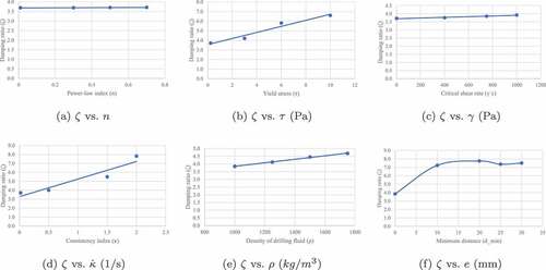
Through further simulations, it was identified that the damping ratio also depends on the combined effect of eccentricity (e) and the wellbore diameter ($r_{well}$). The minimum distance between the drill pipe and the wellbore ($d_{min}$), which is a derived variable of (e) and ($r_{well}$), was considered important. It is presented in Equation 5(5) $d_{min}=r_{well}-r_{pipe}-e$(5) . The individual effect on the damping ratio of each variable is illustrated in Figure 2. They were evaluated through FSI simulations for non-Newtonian fluids.

(4) $\zeta =f(\kappa ,\tau ,v,d_{min},\rho )$(4)

(5) $d_{min}=r_{well}-r_{pipe}-e$(5)

In summary, the simulations were performed according to Table 2, and the results for $\zeta$ and ${\omega }_n$ were determined using the method described in Section 1.1.4. The FSI simulations were done using ANSYS® Workbench, while the Response Surface Method (RSM) was used to analyse the data statistically. Design-Expert^TM 13 software was used to design the experiment grid and analyse the results. All the FSI simulations were done using the high-performance computing resources provided by ACENET Canada. The results are presented in the last two columns of Table 2. A similar approach was taken in developing the axial drag model. Therefore, only the results of axial drag, and not the detailed steps, are presented in the interest of brevity.

Table 2. Experiments and the respective results.

$Sim$	$d_{min}$	$\tau$	$\kappa$	$\rho$	$v$	$e$	$\zeta$	$F$
1	36.46	10	0	1750	1.5	0	14.02	12.91
2	21.46	5	1	1000	0.8	15	11.54	9.34
3	36.46	0	0	1000	0.1	0	4.45	0.00
4	6.46	10	2	1750	1.5	30	23.49	65.19
5	6.46	0	2	1750	0.1	30	17.30	11.50
6	6.46	10	0	1750	0.1	30	16.96	8.51
7	21.46	5	1	1750	0.8	15	11.86	9.03
8	21.46	5	1	1375	0.8	15	11.83	9.15
9	36.46	0	2	1000	1.5	0	7.93	162.14
10	6.46	10	2	1750	0.1	30	22.14	20.08
11	21.46	5	0	1375	0.8	15	9.34	2.76
12	6.46	0	2	1750	1.5	30	19.47	81.20
13	21.46	10	1	1375	0.8	15	13.90	5.14
14	36.46	10	2	1750	0.1	0	14.02	29.59
15	36.46	10	0	1000	0.1	0	8.95	12.82
16	36.46	10	0	1000	1.5	0	12.69	17.25
17	6.46	0	2	1000	0.1	30	17.34	11.52
18	36.46	0	0	1750	1.5	0	8.37	2.97
19	21.46	5	1	1375	0.8	15	11.83	9.22
20	6.46	10	2	1000	1.5	30	15.58	62.52
21	6.46	0	0	1750	1.5	30	8.37	2.97
22	21.46	5	1	1375	0.8	15	11.83	9.23
23	6.46	10	2	1000	0.1	30	23.20	20.08
24	6.46	0	2	1000	1.5	30	14.47	67.26
25	21.46	5	1	1375	0.8	15	11.83	9.23
26	36.46	0	2	1000	0.1	0	17.34	11.52
27	36.46	0	0	1750	0.1	0	8.33	0.02
28	36.46	5	1	1375	0.8	0	14.45	20.91
29	21.46	5	1	1375	0.1	15	14.07	7.65
30	21.46	5	1	1375	0.8	15	11.83	9.23
31	6.46	5	1	1375	0.8	30	14.45	20.93
32	36.46	0	2	1750	0.1	0	17.30	11.51
33	6.46	0	0	1000	1.5	30	7.26	1.70
34	6.46	10	0	1000	1.5	30	12.69	17.27
35	36.46	10	0	1750	0.1	0	16.96	8.52
36	21.46	5	1	1375	0.8	15	11.83	9.23
37	6.46	0	0	1750	0.1	30	8.33	0.02
38	36.46	10	2	1750	1.5	0	11.91	178.88
39	36.46	0	2	1750	1.5	0	9.51	175.48
40	21.46	5	1	1375	0.8	15	11.83	9.23
41	36.46	10	2	1000	1.5	0	7.59	165.65
42	21.46	5	2	1375	0.8	15	14.28	23.30
43	36.46	10	2	1000	0.1	0	13.57	28.84
44	21.46	5	1	1375	0.8	15	11.83	9.23
45	6.46	0	0	1000	0.1	30	7.25	0.01
46	6.46	10	0	1750	1.5	30	12.94	26.18
47	6.46	10	0	1000	0.1	30	17.74	8.53
48	36.46	0	0	1000	1.5	0	4.21	0.71
49	21.46	0	1	1375	0.8	15	11.54	9.37
50	21.46	5	1	1375	1.5	15	11.00	9.23

2.1.1. Approximation of the continuous FSI simulation element to a lumped segment system element

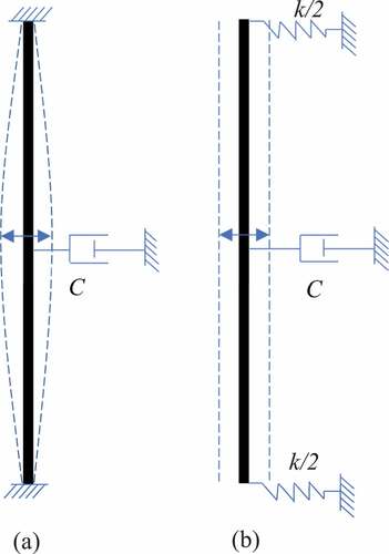
The FSI simulation and the lumped segment model, illustrated in Figure 3. $a$ and $b$ respectively, can be considered as approximately equivalent for lateral vibration damping. Figure 3. $a$ represents a flexible body while Figure 3. $b$ represents a rigid body. Both the bodies oscillate with small amplitudes in comparison with their lengths. For example, the length of the beam is approximately $10m$ while the maximum amplitude is around $10mm$. Therefore, the movement of the two ends can be neglected and hence can be approximated to a fixed-fixed case.

Figure 3. The approximation to a spring-mass-damper system.

2.1.2. The FSI simulation

Moreover, the maximum angular oscillation is approximately 1 degree for a given drill pipe in operation. This is applicable for most of the drill pipe-wellbore radii combinations. Therefore, the angular orientation effect on lateral damping can be neglected. Hence, this small vibration amplitude assumption allows the flexible body oscillation to be approximated to a translational lumped segment spring-mass-damper system. Based on this approximation, the damper with damping constant $C$ is employed to represent the damping experienced by the flexible body, while the effective stiffness of the springs ($k$) represents the bending stiffness of the flexible body. This approximation is further justified in Section 4.

The bending stiffness is defined as the force required to laterally displace the midpoint of the flexible beam by a unit displacement. One can argue that the fixed-fixed boundary condition may be too rigid to simulate the actual dynamics of the drill pipe, and instead, a flexible boundary condition is more appropriate. Nevertheless, the fixed-fixed boundary conditions were introduced to establish the computational stability of the FSI simulation as there are still some limitations that exist in commercial software, in the domain of FSI simulations, at the time of these experiments.

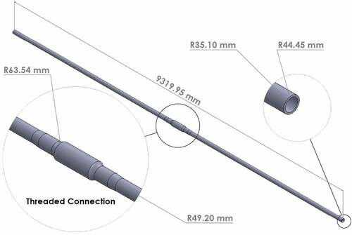
The structural part of the FSI simulation consists of a threaded connection of two drill pipes and two half lengths of the respective pipe as shown in Figure 4. This is taken as the repeating unit of the BG lumped segment simulation presented in Section 3. The fixed-fixed boundary condition provides a sufficient approximation to actual scenarios where the clearance between the wellbore and the drill string is small in comparison with the length of the structure as described in 4. The material assigned is Structural Steel with Young’s Modulus of 2 $\times$ 10¹¹ Pa. The time step for the simulation was 0.03 s. Grid dependency tests were done for the structural and fluid simulation meshes separately. The number of elements was doubled and was checked the consistency of the damping ratio ($\zeta$). Hex dominant method was used for both the domains while keeping the element quality above 0.5. As excitation, an impulse was given at the mid-span of the beam with a maximum amplitude of 100 N.

Figure 4. Repeating unit of the lumped segment model.

On the other hand, there are two separate fluid bodies in the fluid flow simulation: the pipe flow and the annular flow. The two flows are concurrent, resembling the fluid flow in an actual drilling process. In Fluent®, the k-omega viscous model was used, and a new fluid was defined to meet the rheology of the drilling fluid. The density ($\rho$), Consistency Index ($\kappa$), and Yield Stress Threshold ($\tau$) were defined according to the respective experiment listed in Table 2. The Power-low Index ($n$) was kept at 0.7, while the Critical Shear Stress (${\dot{\gamma }}_c$) was kept at 10 due to the lack of contribution to the damping effect in the range considered. The Herschel Bulkley model was used to simulate the drilling fluid by activating the turbulent non-Newtonian feature of ANSYS® Fluent (i.e. turb-non-Newtonian) [36].

In defining the boundary conditions of the fluid domains, the inlets of both the pipe and the annulus were given velocity inlet conditions while the outlets were set as pressure outlets. Also, the structural body’s inner and outer surfaces were set as stationary walls with no-slip shear conditions. The surfaces that touch the structural body’s inner and outer surfaces were defined as dynamic mesh zones.

After setting up the structural and fluid simulations, System Coupling is used to communicate between the two domains. Setting up the data transfer between the domains is the key step of this section. Here a two-way data transfer should be implemented: between the annular flow and the outer surface of the structural body, and between the pipe flow and the inner surface of the structural body. Further, the time step must be consistent between the structural and fluid simulations.

Finally, the setup applications of TS and Fluent are connected to the setup of System Coupling to synchronize the individual solvers, manage data transfers between solvers, and monitor the overall convergence of the FSI solution.

In summary, a fluid-solid interface on surfaces is defined in ANSYS® Structural, and it identifies surfaces in the structural model that accept fluid forces from the CFD analysis. Meanwhile, in ANSYS® Fluent, a dynamic mesh zone is defined while it identifies surfaces in the CFD model that accept the motion from the calculated structural deformations. The System Coupling also plays a major role by synchronizing the individual solvers while managing data transfers between solvers and monitoring the FSI solution’s overall convergence.

2.1.3. Analysis of data

The secondary and the most important application of Design Expert software is the statistical analysis of the experimental results. The quality of the model is evaluated based on the analysis of variance (ANOVA) including $R^2$ and lack of fit. These results are presented in Table 3. Figure 5 illustrates the scatter plot of the predicted values versus the actual values. According to the analysis results, $R^2$ was 0.97 while the Predicted $R^2$ is 0.80. The latter is in reasonable agreement with the Adjusted $R^2$ of 0.94 as their difference is less than 0.2. The Adequate Precision Ratio measures the signal-to-noise ratio. It was estimated as 20.5, where a ratio greater than 4 is desirable. In other words, it indicates an adequate signal. The backward elimination method was used in refining the model terms to get a better approximation. Equation 6(6) $\begin{array}{cc}\hspace{0.17em}& \zeta =+12.54627-0.693954d_{min}-0.084\tau \\ \hspace{0.17em}& +4.24983\kappa -0.001892\rho -2.20353v\\ \hspace{0.17em}& +0.042799d_{min}\tau +0.184160d_{min}\kappa \\ \hspace{0.17em}& +0.000276d_{min}\rho +0.157667d_{min}v\\ \hspace{0.17em}& -0.115017\tau \kappa -0.357980\tau v\\ \hspace{0.17em}& +0.000089\kappa \rho -3.34267\kappa v\\ \hspace{0.17em}& +0.001447\rho v+0.006495d_{min}^2\\ \hspace{0.17em}& +0.109795{\tau }^2-0.007902d_{min}\tau \kappa \\ \hspace{0.17em}& +0.014765d_{min}\tau v-0.000118d_{min}\kappa \rho \\ \hspace{0.17em}& -0.083163d_{min}\kappa v-0.000127d_{min}\rho v\\ \hspace{0.17em}& +0.002956\kappa \rho v-0.005616d_{min}{\tau }^2\end{array}$(6) and Figure 6 represent the mathematical model generated through the statistical analysis using Design-Expert^TM.

Figure 5. $\zeta$- Predicted vs. actual.

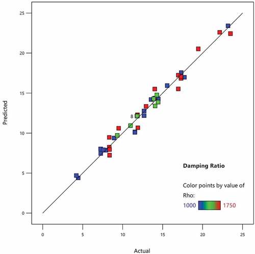
Figure 6. Damping ratio model.

(6) $\begin{array}{cc}\hspace{0.17em}& \zeta =+12.54627-0.693954d_{min}-0.084\tau \\ \hspace{0.17em}& +4.24983\kappa -0.001892\rho -2.20353v\\ \hspace{0.17em}& +0.042799d_{min}\tau +0.184160d_{min}\kappa \\ \hspace{0.17em}& +0.000276d_{min}\rho +0.157667d_{min}v\\ \hspace{0.17em}& -0.115017\tau \kappa -0.357980\tau v\\ \hspace{0.17em}& +0.000089\kappa \rho -3.34267\kappa v\\ \hspace{0.17em}& +0.001447\rho v+0.006495d_{min}^2\\ \hspace{0.17em}& +0.109795{\tau }^2-0.007902d_{min}\tau \kappa \\ \hspace{0.17em}& +0.014765d_{min}\tau v-0.000118d_{min}\kappa \rho \\ \hspace{0.17em}& -0.083163d_{min}\kappa v-0.000127d_{min}\rho v\\ \hspace{0.17em}& +0.002956\kappa \rho v-0.005616d_{min}{\tau }^2\end{array}$(6)

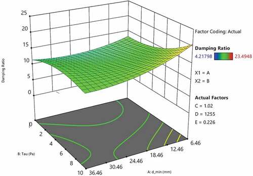
Table 3. ANOVA for reduced cubic model.

Source	Sum of Squares	df	Mean Square	F-value	p-value
Model	882.42	23	38.37	39.83	< 0.0001
A-d_min	1.137E-13	1	1.137E-13	1.180E-13	1.0000
B-Tau	142.48	1	142.48	147.92	< 0.0001
C-K	225.37	1	225.37	233.98	< 0.0001
D-Rho	41.36	1	41.36	42.94	< 0.0001
E-v	56.25	1	56.25	58.40	< 0.0001
AB	16.07	1	16.07	16.69	0.0004
AC	50.65	1	50.65	52.59	< 0.0001
AD	3.28	1	3.28	3.41	0.0764
AE	2.36	1	2.36	2.45	0.1294
BC	64.79	1	64.79	67.27	< 0.0001
BE	0.6626	1	0.6626	0.6880	0.4144
CD	0.0250	1	0.0250	0.0260	0.8732
CE	17.73	1	17.73	18.41	0.0002
DE	6.25	1	6.25	6.49	0.0171
A^2	7.76	1	7.76	8.05	0.0087
B^2	0.2610	1	0.2610	0.2709	0.6071
ABC	11.24	1	11.24	11.67	0.0021
ABE	19.23	1	19.23	19.96	0.0001
ACD	14.05	1	14.05	14.59	0.0007
ACE	24.40	1	24.40	25.33	< 0.0001
ADE	7.96	1	7.96	8.27	0.0079
CDE	19.26	1	19.26	20.00	0.0001
AB^2	8.35	1	8.35	8.67	0.0067
Residual	25.04	26	0.9632
Lack of Fit	25.04	19	1.32
Pure Error	0.0000	7	0.0000
Cor Total	907.46	49

2.2. Axial drag model

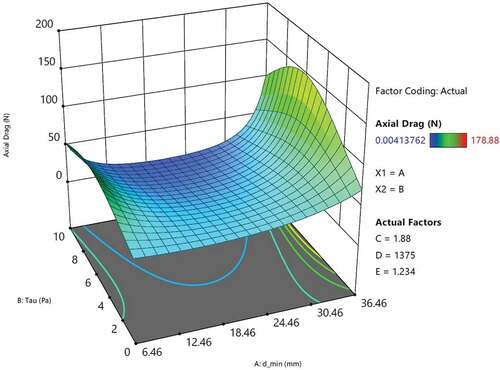
The DoE with statistical analysis approach used to develop the lateral damping model was utilized to establish the axial drag force model. The same set of FSI simulations was utilized to extract the axial drag force using a Probe tool in ANSYS® Transient Structural. Figure 7 illustrates the scatter plot of the predicted values versus the actual values. The mathematical model generated through the statistical analysis using Design-Expert^TM is presented as Equation 7(7) $\begin{array}{cc}\hspace{0.17em}& \sqrt{\frac{1}{F_{axial}+6}}=0.458515-0.008247d_{min}\\ \hspace{0.17em}& -0.038522\tau -0.082539\kappa +1.1\times {10}^{-6}\rho \\ \hspace{0.17em}& -0.091565+0.002308d_{min}\tau \\ \hspace{0.17em}& -0.000031d_{min}\kappa -2.1\times {10}^{-7}{d}_{min}\rho \\ \hspace{0.17em}& +0.009765d_{min}v+0.006870\tau \kappa \\ \hspace{0.17em}& +1.01\times {10}^{-6}\tau \rho -0.000888\tau v\\ \hspace{0.17em}& +1.4\times {10}^{-6}\kappa \rho -0.035233\kappa v\\ \hspace{0.17em}& -0.000028\rho v+0.000201d_{min}^2\\ \hspace{0.17em}& +0.000949{\tau }^2+{0.020037}^2\\ \hspace{0.17em}& +{1.1342110}^{-7}{d}_{min}\tau \rho \\ \hspace{0.17em}& +0.000058d_{min}\tau v-0.000650d_{min}\kappa v\\ \hspace{0.17em}& -1.6\times {10}^{-6}\tau \kappa \rho +0.001970\tau \kappa v\\ \hspace{0.17em}& +0.000012\kappa \rho v-0.000059d_{min}^2\tau \\ \hspace{0.17em}& -0.000219d_{min}^{2}v\end{array}$(7) and Figure 8. As depicted in Figure 8, the increasing $\tau$ has a considerably high effect on the axial drag.

Figure 7. Drag force: predicted vs. actual.

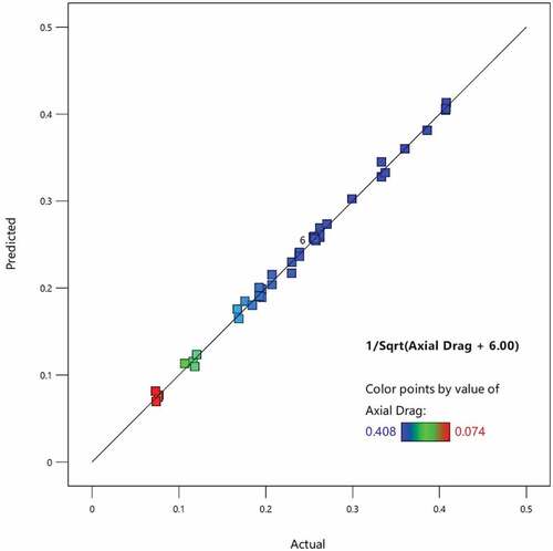
Figure 8. Axial drag model.

In refining the model terms, the Backward Elimination Method was followed to get the best-fit statistics. The $R^2$ was 0.99 while the Predicted $R^2$ of 0.97 was in reasonable agreement with the Adjusted $R^2$ of 0.99. The Adequate Precision Ratio was estimated as 67 which indicates an adequate signal. Equation 7(7) $\begin{array}{cc}\hspace{0.17em}& \sqrt{\frac{1}{F_{axial}+6}}=0.458515-0.008247d_{min}\\ \hspace{0.17em}& -0.038522\tau -0.082539\kappa +1.1\times {10}^{-6}\rho \\ \hspace{0.17em}& -0.091565+0.002308d_{min}\tau \\ \hspace{0.17em}& -0.000031d_{min}\kappa -2.1\times {10}^{-7}{d}_{min}\rho \\ \hspace{0.17em}& +0.009765d_{min}v+0.006870\tau \kappa \\ \hspace{0.17em}& +1.01\times {10}^{-6}\tau \rho -0.000888\tau v\\ \hspace{0.17em}& +1.4\times {10}^{-6}\kappa \rho -0.035233\kappa v\\ \hspace{0.17em}& -0.000028\rho v+0.000201d_{min}^2\\ \hspace{0.17em}& +0.000949{\tau }^2+{0.020037}^2\\ \hspace{0.17em}& +{1.1342110}^{-7}{d}_{min}\tau \rho \\ \hspace{0.17em}& +0.000058d_{min}\tau v-0.000650d_{min}\kappa v\\ \hspace{0.17em}& -1.6\times {10}^{-6}\tau \kappa \rho +0.001970\tau \kappa v\\ \hspace{0.17em}& +0.000012\kappa \rho v-0.000059d_{min}^2\tau \\ \hspace{0.17em}& -0.000219d_{min}^{2}v\end{array}$(7) and Figure 8 represent the axial drag model.

(7) $\begin{array}{cc}\hspace{0.17em}& \sqrt{\frac{1}{F_{axial}+6}}=0.458515-0.008247d_{min}\\ \hspace{0.17em}& -0.038522\tau -0.082539\kappa +1.1\times {10}^{-6}\rho \\ \hspace{0.17em}& -0.091565+0.002308d_{min}\tau \\ \hspace{0.17em}& -0.000031d_{min}\kappa -2.1\times {10}^{-7}{d}_{min}\rho \\ \hspace{0.17em}& +0.009765d_{min}v+0.006870\tau \kappa \\ \hspace{0.17em}& +1.01\times {10}^{-6}\tau \rho -0.000888\tau v\\ \hspace{0.17em}& +1.4\times {10}^{-6}\kappa \rho -0.035233\kappa v\\ \hspace{0.17em}& -0.000028\rho v+0.000201d_{min}^2\\ \hspace{0.17em}& +0.000949{\tau }^2+{0.020037}^2\\ \hspace{0.17em}& +{1.1342110}^{-7}{d}_{min}\tau \rho \\ \hspace{0.17em}& +0.000058d_{min}\tau v-0.000650d_{min}\kappa v\\ \hspace{0.17em}& -1.6\times {10}^{-6}\tau \kappa \rho +0.001970\tau \kappa v\\ \hspace{0.17em}& +0.000012\kappa \rho v-0.000059d_{min}^2\tau \\ \hspace{0.17em}& -0.000219d_{min}^{2}v\end{array}$(7)

2.3. Validation of the FSI simulation

The main goal of this experiment is to improve the confidence of the FSI simulation, which is used to develop the lateral damping and axial drag models. The simulation was scaled down to match the laboratory scale model, and the experimental results were compared with the simulation results.

2.3.1. Laboratory apparatus and experiment procedure

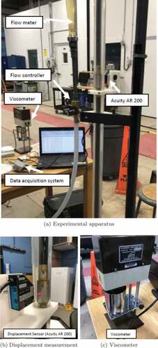
The apparatus used in the experimental work was first designed in SolidWorks as shown in Figure 9 while the fabricated model is shown in Figure 10. Fluid driven by a centrifugal pump enters the inner vertical pipe through the inlet ($A$) at the top, fills the chamber at the bottom ($C$) and rises through the annulus. The inner pipe can be excited using a permanent magnet placed at the steel fitting ($F$), which resembles the drill string threaded connection. The oscillation is captured using a laser displacement sensor (i.e. Acuity AR 200) and the data acquisition system.

Figure 9. The 3D CAD model of the apparatus.

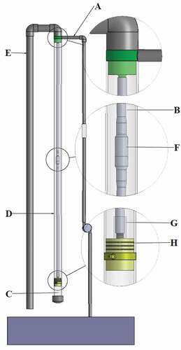
Figure 10. Experimental apparatus and equipment used.

The experiment was performed for Newtonian and non-Newtonian fluids separately. For the Newtonian fluid case, the apparatus was directly connected to the laboratory water supply, which can drive water with a maximum rate of $3.7\times {10}^{-4}{m}^3/s$. The method presented in 1.1.4 was used to estimate the damping ratios while the respective steady flow velocities were determined using the flow metre reading. A sample reading taken using Acuity AR 200 is shown in Figure 11. The results are illustrated in Figure 12 along with the simulation results.

Figure 11. Sample experimental data.

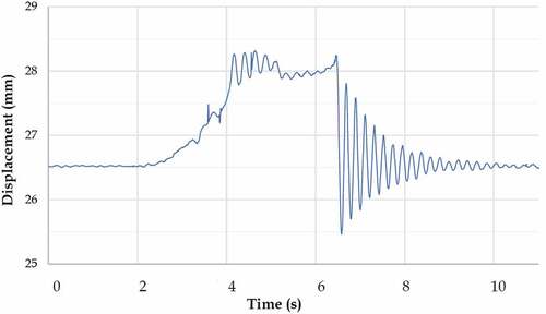
Figure 12. Damping ratio change in Newtonian fluid.

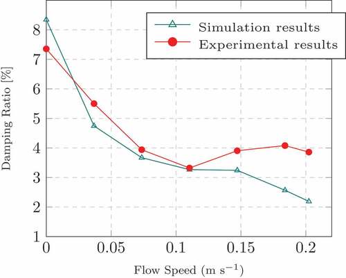
The non-Newtonian fluid was made using 30 $g$ of Xanthan Gum dissolved in 100 litres of water. The rheological properties of the fluid were determined using the OFITE model 800 viscometer shown in Figure 10c. The shear stress versus shear rate curve determined using the viscometer is illustrated in Figure 13. A centrifugal pump of 372 $W$ was used to drive the fluid through the apparatus. Damping measurements were taken following the same procedure used in the Newtonian fluid case. The experimental and simulation results are presented in Figure 14.

Figure 13. Viscometer test results of the non-Newtonian fluid.

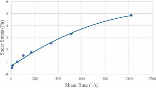
Figure 14. Damping ratio change in non-Newtonian fluid.

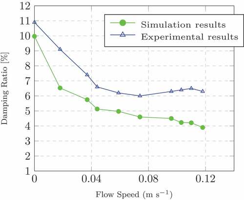
The experimental and the simulation results are in reasonable agreement for both Newtonian and non-Newtonian fluids as shown in Figures 12 and 14. The experimental curves in both cases at lower speeds show a reduction of the damping ratio with increasing flow speed which is also reflected in the simulation result. However, the experimental results corresponding to the second half of the speed range indicate an increase of the damping ratio, which is not evident in the simulation results. Nevertheless, the simulation can capture the overall reduction of the damping ratio with increasing fluid speed. The technical difficulties faced in FSI simulations and techniques used to overcome them are discussed in Section 4.

3. Case study and results

The damping and drag models were implemented in a 3D multi-segment bond graph. The damping ratio ($\zeta$) changes continuously depending on the respective values of $\kappa$, $\tau$, $v$, $d_{min}$, and $\rho$. The lateral damping model presented in Equation 6(6) $\begin{array}{cc}\hspace{0.17em}& \zeta =+12.54627-0.693954d_{min}-0.084\tau \\ \hspace{0.17em}& +4.24983\kappa -0.001892\rho -2.20353v\\ \hspace{0.17em}& +0.042799d_{min}\tau +0.184160d_{min}\kappa \\ \hspace{0.17em}& +0.000276d_{min}\rho +0.157667d_{min}v\\ \hspace{0.17em}& -0.115017\tau \kappa -0.357980\tau v\\ \hspace{0.17em}& +0.000089\kappa \rho -3.34267\kappa v\\ \hspace{0.17em}& +0.001447\rho v+0.006495d_{min}^2\\ \hspace{0.17em}& +0.109795{\tau }^2-0.007902d_{min}\tau \kappa \\ \hspace{0.17em}& +0.014765d_{min}\tau v-0.000118d_{min}\kappa \rho \\ \hspace{0.17em}& -0.083163d_{min}\kappa v-0.000127d_{min}\rho v\\ \hspace{0.17em}& +0.002956\kappa \rho v-0.005616d_{min}{\tau }^2\end{array}$(6) was implemented in the bond graph model as a modified R element. The drag force model presented in Equation 7(7) $\begin{array}{cc}\hspace{0.17em}& \sqrt{\frac{1}{F_{axial}+6}}=0.458515-0.008247d_{min}\\ \hspace{0.17em}& -0.038522\tau -0.082539\kappa +1.1\times {10}^{-6}\rho \\ \hspace{0.17em}& -0.091565+0.002308d_{min}\tau \\ \hspace{0.17em}& -0.000031d_{min}\kappa -2.1\times {10}^{-7}{d}_{min}\rho \\ \hspace{0.17em}& +0.009765d_{min}v+0.006870\tau \kappa \\ \hspace{0.17em}& +1.01\times {10}^{-6}\tau \rho -0.000888\tau v\\ \hspace{0.17em}& +1.4\times {10}^{-6}\kappa \rho -0.035233\kappa v\\ \hspace{0.17em}& -0.000028\rho v+0.000201d_{min}^2\\ \hspace{0.17em}& +0.000949{\tau }^2+{0.020037}^2\\ \hspace{0.17em}& +{1.1342110}^{-7}{d}_{min}\tau \rho \\ \hspace{0.17em}& +0.000058d_{min}\tau v-0.000650d_{min}\kappa v\\ \hspace{0.17em}& -1.6\times {10}^{-6}\tau \kappa \rho +0.001970\tau \kappa v\\ \hspace{0.17em}& +0.000012\kappa \rho v-0.000059d_{min}^2\tau \\ \hspace{0.17em}& -0.000219d_{min}^{2}v\end{array}$(7) and the upthrust were also implemented in the effort source (Se) as a modification to the weight.

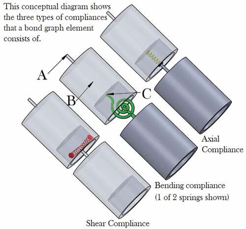
The bond graph consists of 22 of the repeating units depicted in Figure 4. The drill string is fixed at both ends through stiff lateral displacement springs with damping in parallel to remove high frequency transients. An expanded bond graph element is illustrated in Figure 15 while Figure 16 illustrates the bond graph construction at the interface of two elements. The function of each sub-model is described in the figures, while the simulation files can be accessed through the author’s https://github.com/mihiranpathmika/Bond-graph-simulations.gitonline repository [37]. The three different compliances (i.e. axial, bending, and shear) and the points A, B, and C of a given BG element are illustrated in Figure 17. Further information on the development of the bond graph is available in [10] and [6].

Figure 15. 3D bond graph element.

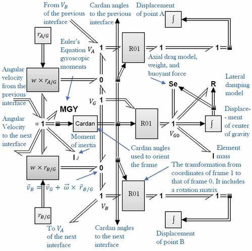
Figure 16. Interface between elements.

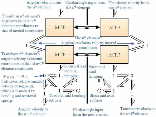
Figure 17. BG element compliances.

The bond graph has a mass imbalance created at the 11th element while an impulse is given at the 10^th element. The drill string is rotated with a modified effort source with a PID controller to generate the top drive speed at the first element. Therefore, this bond graph represents a rotating drill string connected to the top drive, which interacts with the wellbore wall. This helps to identify the effect of the damping constant on the bending movement fluctuation.

The interaction with the well bore is detected using a modified capacitive element which resembles stiff springs come in to contact with the BG element when it reaches the well bore. The schematic of a contact spring with a stiffness of $k_w$ is illustrated in Figure 18. The stiff spring with discontinuous constitutive laws provide no effort until the eccentricity $e$ exceeds the radial clearance between the well bore and the drill pipe. Further details and relevant equations are presented in [10].

Figure 18. Contact spring schematic [10].

The minimum distance $d_{min}$ is a real-time measurement calculated using the lateral displacement of the respective element. As illustrated in Figure 3, the damper (R element) was connected at the centre of the bond graph element. The lateral displacement is determined by integrating the midpoint velocity. Here the damping constant is the multiplication of the critical damping constant ($C_c$) and the damping ratio determined by the model. 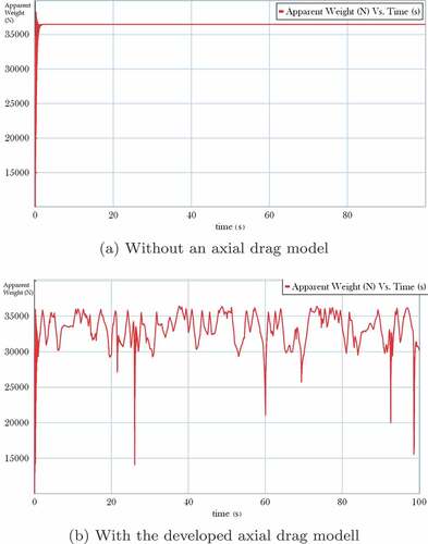The critical damping constant $(C_c)=2\sqrt{km}$ where k is the bending stiffness and m is the element’s mass. A separate bond graph was developed with constant damping and drag forces. A comparison of the bending moment and axial drag force fluctuations of the models is provided in Figures 19 and 20 respectively.

Figure 19. Bending moment fluctuation.

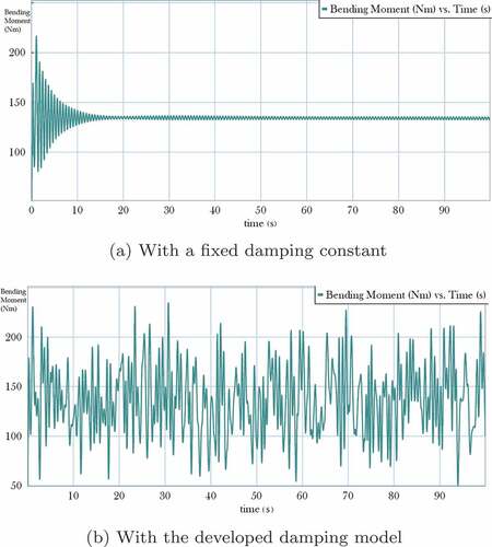
Figure 20. Drill string’s apparent weight fluctuation.

3.1. Buoyant force model

To complete the evaluation of forces due to drilling fluid, the upthrust or the buoyant force is determined using the fundamental equation of Archimedes’ principle (i.e. U = V $\rho$ g) where $V$ is the immersed volume of the element, $\rho$ is the density of the drilling fluid, and $g$ is the gravitational acceleration. If the drill string element is fully immersed, $V$ will be constant. It states that the buoyant force is equal to the weight of the displaced fluid by a fully or partially immersed body. Therefore, the change in density of the drilling fluid is the only variable as the change in gravity $g$ with the depth is insignificant with reference to the other forces.

4. Discussion

Although there are numerous examples of drill string models in the literature, a study regarding the effect of fluctuating fluid forces on drill strings is rare. Most of the available models do not consider all the contributing variables to the lateral damping and axial drag effects. This study develops and implements a damping model and an axial drag model, considering drilling fluid rheology and the location of the drill string in the wellbore.

Lumped segment models in general consist of rigid bodies connected together with springs and dampers. The FSI simulation used in this study consists of an elastic beam with fixed-fixed end conditions which is still a fair approximation for the following reasons. The lumped segment model element is 10 m in length which resembles an API 5D drill pipe connection beneath two half pipe segments. It is the repeating unit of the lumped segment model shown in Figure 4. The wellbore radial clearance is 36 mm in the case study. Therefore, the rotation of the segment about a lateral axis is approximately $1^{\circ }$ and can be neglected. Also, the angle is less than ${10}^{\circ }$ for most of the well bore-drill pipe combinations. Furthermore, lateral damping occurs due to the sweeping action of the drill pipe through the drilling fluid. Being a low amplitude vibration, the amount of fluid with which the string interacts in both Figures 3a,b are almost equal. In other words, the sum of distance travelled against the fluid friction by each of the small elements in the respective segment in Figures 3a,b are approximately equal which leads to a similar energy dissipation given that $\mathrm{\Delta }{x}_1$ is greater than $\mathrm{\Delta }{x}_2$.

The drilling fluid is assumed to behave according to the Hershel-Bulkley model in the FSI simulations used. The viscometer test results indicate that the fluid used in the physical experiment also follows the same model as shown in Figure 13. Nevertheless, the presence of the rock cuttings is considered neither in the simulation nor in the physical experiment, and the drilling fluid is considered a continuum. The relationship between the cutting size distribution and the damping ratio is an open research topic.

The numerical simulation has some limitations when a softer material is used in the structural domain. When the structure material is softer than steel and the density is comparatively low, the added mass effect on the structure’s vibration makes the solver unstable, leading to the termination of the simulation. This is a known limitation of the CFD code [38,39] as of the time of this publication. Note that the link of the citations [38,39] can be accessed through ANSYS® help only. Therefore, the structural material was selected as steel, and its elastic modulus was manually decreased gradually to find the critical stiffness of the material, which is case-specific, that can run a stable simulation for the current model. It was found that the critical stiffness is 7.5 $GPa$, nearly 7.5 times that of the physical model made out of Polyethylene (PE). An approximate damping ratio can then be determined from the FSI simulation using logarithmic decrement. As the lateral damping is mainly governed by the work done against the fluid friction, and given that the geometry of the stiffer pipe is identical to that of the actual, the damping ratio was assumed to be approximately equal for lower amplitude vibrations. To improve the confidence of this assumption, the damping ratio of a steel drill pipe connection with a stiffness of 200 $GPa$ was compared against a steel drill pipe with a modified stiffness of 1500 $GPa$. The stiffer pipe showed a 5–10% reduction in damping ratio compared to the other. This can be due to the shear-thinning nature of the drilling fluid and the excessive vibration frequency of the stiffened structure.

As a solution for this technical limitation of FSI simulations with softer materials, the use of the Quasi-Newton Stabilization Algorithm and Solution Stabilization option is recommended [38,39]. Instead of using ANSYS® Workbench for the coupling analysis, the command prompt was used to integrate Transient Structural, Fluent, and System Coupling applications where the Quasi-Newton Stabilization Algorithm is accessible. Alternatively, a manual tuning using the Solution Stabilization option was done. Both attempts were not successful in ANSYS® 2021 R2, and ANSYS® 2022.

Although there is not much effect on the vibration amplitude decay, the elastic modulus increase causes mismatches in the damping ratio and natural frequencies. When the vibration amplitude is in the 0 to 1 $mm$ range, the effect of the boundary layer adjacent to the pipe’s outer surface becomes considerable compared to higher amplitude cases. It can cause differences between the experimental and simulation results. On the other hand, the stiffer structure shows a higher natural frequency as expected. Therefore, the natural frequency of the simulation results shows a higher value compared to that of the experimental results. Further, as shown in Figure 21, the natural frequency becomes stable after 0.075 $m{s}^{-1}$. This transition occurs when the annular flow reaches the critical Reynold’s number that can be verified based on the findings of [40]. According to [40], the critical Reynold’s number for the radius ratio can be approximately estimated as 2350, referring to Figure 22. On the other hand, Reynold’s number for the flow velocity of 0.075 $m{s}^{-1}$, where the transition occurs, can be calculated using Equation 8(8) $Re=\frac{2U\rho (R_1-R_2)}{\mu }$(8) . It was found that both Reynold’s numbers are almost equal. This verifies that the variation of natural frequency is due to the transition from laminar to turbulent flow.

(8) $Re=\frac{2U\rho (R_1-R_2)}{\mu }$(8)

Figure 21. Natural frequency vs. fluid velocity.

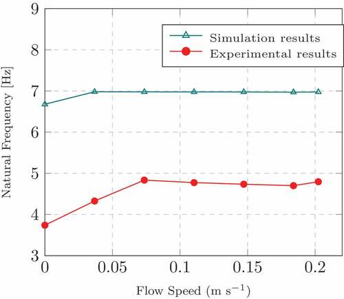
Figure 22. Radius ratio vs. Reynolds number.[40]

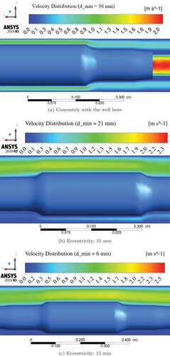
Figure 23 depicts that the variation of fluid velocity inside the annular space with reducing $d_{min}$ or increasing eccentricity $e$. The maximum velocity in the annular region varies with eccentricity, creating changes in the viscous and inertial fluid forces acting on the drill pipe. This verifies the importance of incorporating $d_{min}$ into the damping and drag models.

Figure 23. Velocity distribution with the changing eccentricity (Figures illustrate the change in maximum velocity with increasing eccentricity).

As shown in Figure 19, models with fixed damping constants underestimate the bending moment fluctuation at lower speeds. This becomes critical when the drill string is under stick-slip vibration because the speed goes to the lower extreme periodically. On the other hand, at speeds around 50 rpm, the bond graph model with a fixed damping constant showed greater well bore interaction than the bond graph model with variable damping. This indicates that the implemented damping model captures the effect of the lateral displacement and the drilling fluid properties and brings it into the drill string vibration response. This shows the potential to improve the prediction accuracy of stress fluctuations and wellbore interaction for a given drill pipe, if a continuously variable damping model is used. It will benefit applications such as fatigue life prognosis of drill strings.

Also, this model can estimate the apparent fluctuating weight of the drill string due to the drilling fluid flow. This facilitates estimating fluctuating weight on bit (WoB) of a vertical drill string. For deviated well applications, a friction model can be implemented to bring the contact forces’ contribution into the equation.

In Figure 19a, it can be seen that the amplitude of vibration gradually decays and approaches a fixed value. This is because the drill string is pin joined at the ends, and a mass imbalance comes into action with the implementation of the angular velocity. The mass imbalance pulls the drill string laterally, creating a consistent bend on the entire drill string. Also, the periodic vibration is due to the external impulse given at the 10^th element. Although the same conditions are provided, the second bond graph with the damping model shows a different bending moment fluctuation with a lower decay.

5. Conclusions

A detailed methodology is presented to develop models to determine the instantaneous damping constant and the axial drag force for a given oilwell drill string. The damping models were developed for a drill string with API 5D drill pipes using a series of FSI simulations followed by statistical analysis. The models were implemented in a lumped segment multibody model to demonstrate the importance of treating fluid damping effects with greater complexity than is typical in the literature. Both bending moment fluctuation and the overall axial force is affected by the properties and velocity of the drilling fluid and the instantaneous location of the drill string in the well bore. It was observed that the bending moment fluctuation is underestimated at lower rotational speeds, and the well bore interaction is exaggerated at higher rotational speeds. Therefore, fixed values for the damping constant and axial drag may underestimate important predictions such as remaining useful fatigue life and WoB. Damping and axial drag models developed using the methods of this paper are recommended in drill string lumped-segment simulation models, taking in to account the drilling fluid rheology, instantaneous location of the drill string in the wellbore, drill pipe geometry, and the drilling fluid velocity.

6. Further work

The numerical values in damping model presented in this study apply only to the geometry of an API 5D drill pipe. Further studies can be made to develop a technique to adopt the current models to other drill pipe geometries without requiring a total re-derivation of the model. This can be achieved by performing a series of simulations for different diameters. The outcome may be a chart that can determine a modifying factor for the current models, eliminating or reducing the FSI simulations, which are highly time-intensive.

The shape of the damping curve for increasing velocity indicates a characteristic shape for both Newtonian and non-Newtonian fluids as shown in Figures 21 and 14 respectively, which can be further explored. Also, investigating the effect of rock cuttings with different size distributions on the drill string damping will be a valuable contribution. Further, the damping and the axial drag models can be implemented in a directional well model to investigate the changes in vibration behaviours.

This work was financially supported by the Natural Sciences and Engineering Research Council (NSERC) of Canada and Memorial University of Newfoundland, Canada.

Acknowledgments

The authors thankfully acknowledge the continuous support provided by the Drilling Technology Laboratory (DTL) research group and the Mechanical Division of Technical Services at Memorial University of Newfoundland, Canada.

Disclosure statement

No potential conflict of interest was reported by the author(s).

Additional information

Funding

This work was financially supported by the Natural Sciences and Engineering Research Council (NSERC) of Canada and Memorial University of Newfoundland, Canada.

References

- J.J. Bailey and I. Finnie, An analytical study of drill-string vibration, J. Eng. Ind. 82 (5 1960), pp.122–127. 10.1115/1.3663017
- M. Paidoussis, Fluid-structure Interactions: Slender Structures and Axial Flow, Vol. 1, San Diego, USA: Academic Press. 1998. doi:10.3327/jaesj.47.229.
- M. Paidoussis and N.T. Issid, Dynamic stability of pipes conveying fluid, J. Sound Vib. 33 (3) (1974), pp. 267–294. doi:10.1016/S0022-460X(74)80002-7.
- W.R. Tucker and W. Charles, An integrated model for drill-string dynamics, J. Sound Vib. 224 (1) (1999), pp. 123–165. doi:10.1006/jsvi.1999.2169.
- S. Chen, Fluid damping for circular cylindrical structures, Nucl. Eng. Des. 63 (1) (1981), pp. 81–100. doi:10.1016/0029-5493(81)90018-2.
- S. Mejbahul. Modeling and simulation of vibration in deviated wells. PhD thesis, Memorial University of Newfoundland, 2017.
- Q. Qian, L. Wang, and N. Qiao, Vibration and stability of vertical upward-fluid-conveying pipe immersed in rigid cylindrical channel, Acta Mech. Solida Sin. 21 (5) (2008), pp. 331–340. doi:10.1007/s10338-008-0852-z.
- X. Hua Zhu and B. Li, Numerical simulation of dynamic buckling response considering lateral vibration behaviors in drillstring, J. Pet. Sci. Eng. 173 (September 2018) (2019), pp. 770–780. doi:10.1016/j.petrol.2018.09.090.
- P. M.p, L.T. P, S. Prabhakar et al., Dynamics of a long tubular cantilever conveying fluid downwards, which then flows upwards around the cantilever as a confined annular flow, J Fluids Struct 24 (1) (2008), pp. 111–128. doi:10.1016/j.jfluidstructs.2007.07.004.
- G. Rideout, A. Ghasemloonia, F. Arvani, and S. Butt, An intuitive and efficient approach to integrated modelling and control of three-dimensional vibration in long shafts, Int. J. Simul. Process 10 (2) (2015), pp. 163–178. doi:10.1504/IJSPM.2015.070468.
- F. Arvani, D.G.R. Md Mejbahul Sarker, and D.B. Stephen, Design and development of an engineering drilling simulator and application for offshore drilling for MODUs and deepwater environments. Society of Petroleum Engineers - SPE Deepwater Drilling and Completions Conference 2014; Galveston, Texas, USA, 417–433, 2014.
- T.G. Ritto, C. Soize, and R. Sampaio, Non-linear dynamics of a drill-string with uncertain model of the bit-rock interaction, Int J Non Linear Mech 44 (8) (2009), pp. 865–876. doi:10.1016/j.ijnonlinmec.2009.06.003.
- M. Sarker, G. Rideout, and S. Butt, Dynamic model for longitudinal and torsional motions of a horizontal oilwell drillstring with wellbore stick-slip friction, J. Pet. Sci. Eng. 150 (2017), pp. 272–287. doi:10.1016/j.petrol.2016.12.010.
- D. Xie, Z. Huang, M. Yachao, V. Vaziri, M. Kapitaniak, and M. Wiercigroch, Nonlinear dynamics of lump mass model of drill-string in horizontal well, Int. J. Mech. Sci. 174 (2020), pp. 105450. doi:10.1016/j.ijmecsci.2020.105450.
- V.P. Feodos, Vibrations and stability of a pipe when liquid flows through it, Inzhenernyi Sbornik 10 (1951), pp. 69–70.
- H. Ashley and G. Haviland, Bending vibrations of a pipe line containing flowing fluid, J. Appl. Mech. 17 (9 1950), pp.229–232. 10.1115/1.4010122
- F. Niordson, Vibrations of a Cylindrical Tube Containing Flowing Fluid. Kungliga Tekniska Hogskolans, Handlingar (Stockholm): Göteborg Elanders Boktr, 1953.
- S. Chen, M.W. Wambsganss, and J.A. Jendrzejczyk, Added Mass and Damping of a Vibrating Rod in Confined Viscous Fluids. Argonne, Chicago: American Society of Mechanical Engineers, 1976.
- R. Miller, The Effects of Frequency and Amplitude of Oscillation on the Hydrodynamic Masses of Irregular Shaped Bodies. Kingston, USA: University of Rhode Island, 1965.
- R. Chilukuri, Added mass and damping for cylinder vibrations within a confined fluid using deforming finite elements, J Fluids Eng. 109 (09 1987), pp. 283–288. 10.1115/1.3242662
- E. Kjolsing and M. Todd, Damping of a fluid-conveying pipe surrounded by a viscous annulus fluid, J. Sound Vib. 394 (2017), pp. 575–592. doi:10.1016/j.jsv.2017.01.045.
- F. Liang, Y. Qian, Y. Chen, and A. Gao, Nonlinear forced vibration of spinning pipes conveying fluid under lateral harmonic excitation, Int J Appl Mech 13 (9) (2021), pp. 2150098. doi:10.1142/S1758825121500988.
- R.A. Ibrahim, Overview of mechanics of pipes conveying fluids-part I: Fundamental studies, J. Press. Vessel Technol. Trans. ASME. 132 (2010), pp. 0340011–03400132.
- G. Rideout, F. Arvani, S. Butt, and E. Fallahi, Three-dimensional multi-body bond graph model for vibration control of long shafts-application to oilwell drilling. Proc. Integrated Modeling and Analysis in Applied Control and Automation; Athens, Greece, 25–27, 2013.
- H. Qiu, Y. Jianming, S. Butt, and Z. Jinghan, Investigation on random vibration of a drillstring, J. Sound Vib. 406 (2017), pp. 74–88. doi:10.1016/j.jsv.2017.06.016.
- Y. Khulief and H. Al-Naser, Finite element dynamic analysis of drillstrings, Finite Elem. Anal. Des. 41 (13) (2005), pp. 1270–1288. doi:10.1016/j.finel.2005.02.003.
- Y. Khulief, F. Al-Sulaiman, and S. Bashmal, Vibration analysis of drillstrings with string—borehole interaction, Proc Inst Mech Eng C J Mech Eng Sci. 222 (2008), pp. 2099–2110.
- Y. Khulief and F. Al-Sulaiman, Laboratory investigation of drillstring vibrations, Proc Inst Mech Eng C J Mech Eng Sci. 223 (2009), pp. 2249–2262.
- S. Scampoli, High-fidelityfluid-structure interactions, Ansys Adv. 6 (2012), pp. 14–16.
- W. Young, R. Budynas, and A. Sadegh, Dynamic and temperature Stresses. Roark’s Formulas for Stress and Strain, Edition 8, Vol. 7, New York: McGrawHill, 2002, pp. 774.
- M. Douglas, Design and Analysis of Experiments. New Jersey: John Wiley & Sons, 2017.
- M. Islam and L. Lye, Combined use of dimensional analysis and modern experimental design methodologies in hydrodynamics experiments, Ocean Eng. 36 (3–4) (2009), pp. 237–247. doi:10.1016/j.oceaneng.2008.11.004.
- M. Anderson and P. Whitcomb, RSM Simplified: Optimizing Processes Using Response Surface Methods for Design of Experiments. New York: Productivity Press, 2016.
- A. Aydar, Utilization of response surface methodology in optimization of extraction of plant materials, in Statistical Approaches with Emphasis on Design of Experiments Applied to Chemical Processes, V. Silva, ed., chapter 10 IntechOpen , Rijeka, 2018. pp. 160.
- M.R. Riazi, Exploration and Production of Petroleum and Natural Gas. West Conshohocken, PA: ASTM International, 2016.
- Ansys. Ansys FLUENT 12.0 user’s guide - 12.13.19 modeling turbulence with non-Newtonian fluids, 2009.
- M. Galagedarage Don, Github - mihiranpathmika/bond-graph-simulations: Bond graph simulation files with constant damping and the damping model developed.
- Ansys. FSI is not working for soft materials — ANSYS learning forum, 2020. Accessed: 2022 April 10.
- Ansys. 2-way fsi fails during first time step — Ansys learning forum, 2022. Accessed: 2022 April 10.
- H. Dou, B. Khoo, and H. Tsai, Determining the critical condition for turbulent transition in a full-developed annulus flow, J. Pet. Sci. Eng. 73 (1–2) (2010), pp. 41–47. doi:10.1016/j.petrol.2010.05.003.