Modelling and calibration of a five link elastic boom of a mobile concrete pump

ABSTRACT

Large-scale manipulators, such as the boom of a mobile concrete pump, typically rely on lightweight construction to maximize their operational range. As a result, significant elastic deformations occur during operation. Various automation and control applications require computationally fast and accurate mathematical models of the manipulator’s motion. In this work, a mathematical model for the boom of a mobile concrete pump with 5 individual joints is presented. This model takes into account the elastic bending in two directions and the torsion of the boom. To reach a high model accuracy, calibration is required. This is challenging due to the large dimension and the outdoor operation, which makes the accurate measurement of the boom position difficult. A camera-based measurement setup is proposed in this work that is tailored for the considered problem. It is shown by measurements that the model is able to achieve a high accuracy with rather small computational costs.

KEYWORDS:

• large-scale manipulator
• mobile concrete pump
• flexible multibody system
• model calibration
• computer vision
• Euler-Bernoulli
• Saint-Venant

1. Introduction

In recent years, the building industry is facing an increasing demand concerning the reduction of construction times and costs. As a consequence, manufacturers of building machines aim at making their products more efficient. As an example, mobile concrete pumps, which are used to deliver concrete from the cement mixer to the formwork, have reached a working area of up to 80 m and the boom comprises up to 8 individual joints. Since the carrier truck is limited in length and maximum load, the boom is constructed in the form of very lightweight elastic arm segments connected via complex joint mechanisms¹. The large number of joints and the high flexibility of the boom makes the manual control of these machines by human operators a challenging task. Thus, there is an increasing demand for semi-autonomous assistance systems, which help the operator to achieve the best performance of these building machines.

One main path in the development of such assistance systems is to apply modern model-based automation concepts, which rely on computationally efficient, accurate mathematical models. In design studies and the construction of the building machines, no real-time computation is required. Thus, accurate mathematical models in this field are usually based on finite element modelling (see, e.g. [1,2]). In contrast, control and assistance systems require computationally less expensive models that can be executed in real-time while still ensuring a sufficiently high accuracy.

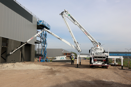
In this work, the boom of a concrete pump with 4 elastic boom elements is considered, see Figure 1. In order to accurately describe the dynamic behaviour of such a machine during motion, the elastic deformations of the lightweight boom have to be systematically taken into account in the mathematical model.

Figure 1. The considered manipulator during operation. picture source: SCHWING GmbH, Heerstrasse 9–27 44653 Herne/Germany.

The mathematical modelling of elastic manipulators is an ongoing research topic, where many works are published in the field of elastic robots, see, e. g the literature review [3] and [4]. In contrast, significantly fewer scientific works can be found that deal with the mathematical modelling of elastic large-scale manipulators, as the boom of the concrete pump studied in this work. The early work [5] motivates the need for accurate mathematical models that cover the full dynamics of the system rather than only allowing for a static approximation of the elastic effects. For large-scale manipulators with comparatively small joint accelerations, the dominating elastic deformation arises from the gravitational force. Most publications focus on this effect only, see, e.g. [6–8], since their main focus is the damping of elastic vibrations in the vertical direction. In [6,7], the Euler-Bernoulli beam theory is employed and the resulting equations of motion are derived using a Ritz approximation with physically motivated ansatz functions. In [8], the equations of motion are also derived by using beam theory while the ansatz functions are obtained from finite element analysis and model order reduction methods. In [9], a boom of a mobile concrete pump is modelled and the elastic deformations including torsional effects are considered using virtual joints, see, e. g. [10]. A similar approach can be found in [11] that uses the technique of virtual flexible joints to describe the elastic deformations of an industrial robot. A research question that is closely related to the mathematical modelling of the boom of a concrete pump is treated in [12], where an elastic model of an aerial ladder was derived. It considers horizontal bending and torsional deformation and describes a vibration damping control based on a modal representation of the first two dominant eigenfrequencies.

The existing mathematical models for the boom of a concrete pump are basically limited to considering the elastic deformations in one direction, i.e. in the direction of gravitation, which is sufficient for the vibration damping control task. During dynamic operation of the boom, however, a significant rotation around the vertical axis can be observed, which induces torsional effects and horizontal bending of the arm elements in addition to the vertical bending. Therefore, the first goal of this work is to develop a computationally efficient mathematical model that accurately captures the dynamic motion of the manipulator, including the joint motions and elastic deformations.

The calibration of the mathematical model by measurements is an important task in order to reach a high model accuracy. For the considered boom of a concrete pump, only coarse knowledge of certain system parameters (e.g. the elasticity of the boom elements) is available. This is due to the fact that a number of elements are attached to the boom (e.g. the pipes for the concrete) which influence the elasticity of the boom and their influence can hardly be accurately estimated from construction data only. While calibration of the dynamic model of industrial robots is quite standard and well described in the literature, the calibration of large-scale manipulators is more difficult due to the problem of accurate position measurement, the large span of the manipulator and the outdoor environment. In [6,8], the calibration problem was solved for a 2-dimensional planar elastic model using computer vision techniques to reconstruct 2-dimensional positions of certain points on the boom. These works showed a high accuracy of vision-based measurements and proved that they are a suitable approach for the calibration of large-scale manipulators. Thus, the second goal of this paper is to extend and apply the ideas of [6] to the model calibration in the full 3-dimensional work space of the boom. This work significantly extends the results of [6] by considering the overall three-dimensional motion of the boom including the elastic deformation of each link in vertical and horizontal direction, and torsional bending motions. Furthermore, a much more elaborate vision-based measurement system for the model validation and calibration is developed and presented in this paper.

The paper is structured as follows: In section 2, the mathematical model is derived, starting with an overview of the considered manipulator and the coordinate frames. In Section 2.1, the kinematics of the rigid-joint elastic-link pairs are described in detail. The discretization of the distributed-parameter system by using Ritz’ method is given in Section 2.2. The equations of motion are derived in Section 2.3 using the Euler-Lagrange formalism. Section 3 deals with the model calibration, where the sensor concept for obtaining real-world data and the calibration process are described in Section 3.1 and Section 3.2. The accuracy of the proposed validated model is finally proven by experiments in Section 3.3.

2. Mathematical model

A sketch of the boom under consideration is depicted in Figure 2. It consists of 5 individual hydraulically actuated rotational joints, where each joint is followed by an elastic link. The first joint (slewing gear) allows a rotation of the boom around the vertical $z_0$-axis, oriented with the negative direction of gravity. The remaining joints 2 to 5 form a planar manipulator in the $x_1{y}_1$-plane. Joint 2 and 3 are actuated using linear hydraulic actuators together with special linkages that transform the linear motion of the actuators to a rotation. Joint 4 and 5 are directly actuated by rotational hydraulic motors. The end effector (i.e. the concrete distribution hose) is attached to the end of link 5. In this work, this hose is not further considered and thus, the end of link 5 is referred to as the end effector. It is obvious that if the task space is given by the 3-dimensional position of the end effector, the manipulator comprises a redundant kinematics of order 2, see, e.g. [13].

Figure 2. Sketch of the considered manipulator, including the used coordinate frames ${\mathrm{\Sigma }}_i$ at $x_i=0,i=1,\dots ,5$.

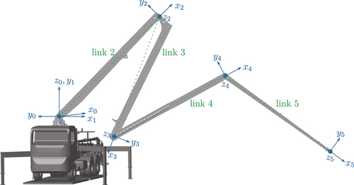
The first link, i.e. the slewing gear, is degenerated to a link with zero length. The links 2 to 5 comprise a lightweight construction which results in significant elastic deformations during the operation of the boom (see, e.g. [8,14]). To account for this elastic deformation, a body-fixed floating coordinate frame ${\mathrm{\Sigma }}_i\left(x_i\right)$ is defined for each link $i$, where the origin and orientation of ${\mathrm{\Sigma }}_i$ is a function of the position $x_i$ at the link due to the elastic deformations. The floating coordinate frames are defined such that $x_i=0$ is located at the end of each link. The inertial coordinate frame ${\mathrm{\Sigma }}_0$ is considered to be rigidly connected to earth.

2.1. Kinematics

The kinematics of each link-joint pair are formulated using two homogeneous transformations, where the first transformation describes the rigid body motion and the second the elastic deformation of the link. This results in a floating frame of reference formulation, see, e.g. [8,15]. The homogeneous representation of a vector ${\mathbf{p}}^i$ is denoted by ${\hat{\mathbf{p}}}^i=[({\mathbf{p}}^i{)}^T,1{]}^T$, where the current reference frame is referred to by the superscript $i$, see [16]. For a shorter notation, the superscript is left out if the vector is represented in the body-fixed coordinate frame. The homogeneous transformation ${\mathbf{H}}_i^{i-1}$ comprises a rotation matrix ${\mathbf{R}}_i^{i-1}\in SO\left(3\right)$ and a translation vector ${\mathbf{d}}_i^{i-1}$, both expressed w. r. t. the coordinate frame ${\mathrm{\Sigma }}_{i-1}$. Therefore, the transformation of a vector ${\mathbf{p}}^i$ defined in the frame $i$ to the frame $i-1$ is given by

(1) ${\hat{\mathbf{p}}}^{i-1}={\mathbf{H}}_i^{i-1}{\hat{\mathbf{p}}}^i={\mathbf{H}}_i^{i-1}\hat{\mathbf{p}},{\mathbf{H}}_i^{i-1}=\left[\begin{array}{cc}{\mathbf{R}}_i^{i-1}& {\mathbf{d}}_i^{i-1}\\ {\mathbf{0}}^{\mathrm{T}}& 1\end{array}\right].$(1)

The relative transformation (rotation and translation) of the rigid body motion of the undeformed links is formulated using a floating representation of the Denavit-Hartenberg (DH) convention, see, e.g. [16], where the DH parameters are functions of the local link coordinate $x_i$. The rigid body transformation from a point located at position $x_i$ of the (undeformed) link $i$ to the origin of joint $i-1$ reads as

(2) ${\bar{\mathbf{H}}}_i^{i-1}=\left[\begin{array}{cccc}{\mathrm{c}}_{q_i}& -{\mathrm{s}}_{q_i}{\mathrm{c}}_{{\kappa }_i}& {\mathrm{s}}_{q_i}{\mathrm{s}}_{{\kappa }_i}& {\lambda }_i\left(x_i\right){\mathrm{c}}_{q_i}\\ {\mathrm{s}}_{q_i}& {\mathrm{c}}_{q_i}{\mathrm{c}}_{{\kappa }_i}& -{\mathrm{c}}_{q_i}{\mathrm{s}}_{{\kappa }_i}& {\lambda }_i\left(x_i\right){\mathrm{s}}_{q_i}\\ 0& {\mathrm{s}}_{{\kappa }_i}& {\mathrm{c}}_{{\kappa }_i}& d_i\left(x_i\right)\\ 0& 0& 0& 1\end{array}\right],$(2)

where the abbreviations ${\mathrm{c}}_{q_i}=cos\left(q_i\right)$, ${\mathrm{s}}_{q_i}=sin\left(q_i\right)$, ${\mathrm{c}}_{{\kappa }_i}=cos\left({\kappa }_i\right)$, ${\mathrm{s}}_{{\kappa }_i}=sin\left({\kappa }_i\right)$ are used. The joint angle is denoted by $q_i$. ${\kappa }_i$ represents the (undeformed) link twist, ${\lambda }_i\left(x_i\right)$ the (undeformed) link length and $d_i\left(x_i\right)$ the (undeformed) link offset at the position $x_i$, see, e.g. [13]. The DH parameters for the links of the considered manipulator are listed in Table 1.

Table 1. Denavit-Hartenberg parameters of the considered manipulator.

$i$	${\lambda }_i\left(x_i\right)$	${\kappa }_i$	$d_i\left(x_i\right)$	$l_i$	$d_i$
				in m
1	0	$\frac{\pi }{2}$	0	0	0
2	$l_2+x_2$	0	$d_2\frac{x_2+l_2}{l_2}$	8.40	−0.17
3	$l_3+x_3$	0	$d_3\frac{x_3+l_3}{l_3}$	7.59	0.24
4	$l_4+x_4$	0	$d_4\frac{x_4+l_4}{l_4}$	7.50	0.74
5	$l_5+x_5$	0	$d_5\frac{x_5+l_5}{l_5}$	7.67	0.02

Note that the offsets in the construction are necessary to avoid link-to-link collisions and thus to allow for a folded configuration of the manipulator. By introducing the dependency of $x_i$ in the translational part of ${\bar{\mathbf{H}}}_i^{i-1}$, a floating frame ${\bar{\mathrm{\Sigma }}}_i\left(x_i\right)$ is defined at each link position $x_i$ of the (undeformed) link $i$, see Figure 3.

Figure 3. Floating coordinate frames and homogeneous transformations from the body fixed frame ${\mathrm{\Sigma }}_i$ to the virtual, rigid body frame ${\bar{\mathrm{\Sigma }}}_i$. Only the links 4 and 5 are depicted compared to Figure 2 and the elastic effects are exaggerated for better visibility.

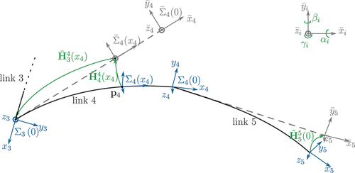
The elastic deformations of the link $i$ at $x_i$ are formulated using a second relative transformation ${\tilde{\mathbf{H}}}_i^i$ w. r. t. the rigid body frame at the same position $x_i$, see Figure 3. It describes the elastic deformations of the neutral axis (stressless line) of the elastic link. The elastic deformations are composed of a torsion around the $x_i$-axis and bending along the orthogonal $y_i$- and $z_i$-directions. Neglecting the warping of the cross-section and denoting the elastic displacement due to bending in the $y_i$- and $z_i$-axis by $v_i$ and $w_i$, respectively, we get the resulting translational displacements ${\tilde{\mathbf{d}}}_i$ in the form

(3) ${\tilde{\mathbf{d}}}_i\left(x_i\right)=\left[\begin{array}{c}0\\ v_i\left(x_i\right)\\ w_i\left(x_i\right)\end{array}\right].$(3)

The elastic deformations also induce a rotation of the link $i$ described by the angles ${\vartheta }_i^{\mathrm{T}}=\left[{\alpha }_i,{\beta }_i,{\gamma }_i\right]$. Here, ${\alpha }_i$ is the torsion angle around the local $x_i$-axis and ${\beta }_i$ and ${\gamma }_i$ are the bending angles around the local $y_i$- and $z_i$-axis, respectively. Based on the Euler-Bernoulli beam theory, they are calculated by

(4a) ${\beta }_i\left(x_i\right)=-arctan\left(\frac{\mathrm{\partial }{w}_i}{\mathrm{\partial }{x}_i}\right)\approx -\frac{\mathrm{\partial }{w}_i}{\mathrm{\partial }{x}_i}$(4a)

(4b) ${\gamma }_i\left(x_i\right)=arctan\left(\frac{\mathrm{\partial }{v}_i}{\mathrm{\partial }{x}_i}\right)\approx \frac{\mathrm{\partial }{v}_i}{\mathrm{\partial }{x}_i},$(4b)

where small displacements are assumed for the simplification in (4). Using again a small angles assumption, i.e. ${\alpha }_i,{\beta }_i,{\gamma }_i\ll 1,$ allows to formulate the rotation matrix ${\tilde{\mathbf{R}}}_i^i\left({\vartheta }_i\right)$ in the form of three consecutive rotations as

(5) ${\tilde{\mathbf{R}}}_i^i\left({\vartheta }_i\right)=\left[\begin{array}{ccc}1& -{\gamma }_i& {\beta }_i\\ {\gamma }_i& 1& -{\alpha }_i\\ -{\beta }_i& {\alpha }_i& 1\end{array}\right]\hspace{0.17em}.$(5)

This allows to represent the homogeneous transformation for the elastic deformation ${\tilde{\mathbf{H}}}_i^i$ as a function of the torsional angle ${\alpha }_i$ and the translational displacements $v_i$, $w_i$ as

(6) ${\tilde{\mathbf{H}}}_i^i=\left[\begin{array}{cc}{\tilde{\mathbf{R}}}_i^i& {\tilde{\mathbf{d}}}_i^i\\ {\mathbf{0}}^{\mathrm{T}}& 1\end{array}\right].$(6)

Combining the homogeneous transformation due to the rigid body motion ${\bar{\mathbf{H}}}_i^{i-1}(x_i)$ with the homogeneous transformation due to the elastic deformation ${\tilde{\mathbf{H}}}_i^i(x_i)$ yields the kinematics for the rigid-joint, elastic-link pair

(7) ${\mathbf{H}}_i^{i-1}(x_i)={\bar{\mathbf{H}}}_i^{i-1}(x_i){\tilde{\mathbf{H}}}_i^i(x_i).$(7)

The overall transformation from link $i-1$ to the end of link $i$ is then given by inserting $x_i=0$ in (7). The overall kinematic chain from the inertial frame to the end effector, which is located in frame 5 at $x_5=0$, is finally calculated by

(8) ${\mathbf{H}}_5^0={\mathbf{H}}_1^0{\mathbf{H}}_2^1{\mathbf{H}}_3^2{\mathbf{H}}_4^3{\mathbf{H}}_5^4{|}_{x_i=0,i=1,\dots ,5}\hspace{0.17em}.$(8)

With this kinematic chain, a general point ${\mathbf{p}}_i$ located at the neutral axis at position $x_i$ of link $i$ is described in the floating coordinate frame ${\mathrm{\Sigma }}_i\left(x_i\right)$ by ${{\mathbf{p}}_i}^{\mathrm{T}}=\left[\begin{array}{ccc}0& 0& 0\end{array}\right]$. Its representation ${\mathbf{p}}_i^0$ in the inertial frame ${\mathrm{\Sigma }}_0$ reads as

(9) ${\hat{\mathbf{p}}}_i^0={\mathbf{H}}_i^0{\hat{\mathbf{p}}}_i,$(9)

where $x_0,\dots ,x_{i-1}=0$ is used in ${\mathbf{H}}_i^0$.

For the subsequent derivation of the equations of motion, the linear velocity ${\mathbf{v}}_i^0$ and the angular velocity ${\omega }_i^0$ of a point ${\mathbf{p}}_i$ relative to the inertial frame are required. They can be calculated by

(10) ${\mathbf{v}}_i^0=\frac{\mathrm{d}}{\mathrm{d}t}{\mathbf{p}}_i^0,({\omega }_i^0{)}^{\mathrm{T}}=\left[{\mathbf{S}}_i^0\left[3,2\right]{\mathbf{S}}_i^0\left[1,3\right]{\mathbf{S}}_i^0\left[2,1\right]\right]$(10)

where ${\mathbf{S}}_i^0[k,l]$ is the entry in row $k$ and column $l$ of the skew-symmetric matrix

(11) ${\mathbf{S}}_i^0=\hspace{0.17em}\frac{\mathrm{d}}{\mathrm{d}t}\left({\mathbf{R}}_i^0\right)\mathbf{R}{ }_i^0{ }^{\mathrm{T}},$(11)

see, e.g. [16].

2.2. Ritz approximation

The elastic degrees of freedom ${\alpha }_i,v_i,w_i$ yield a representation of the dynamical model in the form of a distributed-parameter system, i.e. a model described by partial differential equations. For fast numerical simulations and for using the model in a model-based controller design, a model with low computational complexity, but high accuracy is required. In this work, a Ritz approach is applied, see, e.g. [17], where the elastic degrees of freedom ${\alpha }_i,v_i,w_i$ are approximated by

(12a) ${\alpha }_i\left(x_i,t\right)\approx q_{{\alpha }_i}\left(t\right){\zeta }_{{\alpha }_i}\left(x_i\right)$(12a)

(12b) $v_i\left(x_i,t\right)\approx q_{v_i}\left(t\right){\zeta }_{v_i}\left(x_i\right)$(12b)

(12c) $w_i\left(x_i,t\right)\approx q_{w_i}\left(t\right){\zeta }_{w_i}\left(x_i\right).$(12c)

Here ${\zeta }_{{\alpha }_i}$, ${\zeta }_{v_i}$, ${\zeta }_{w_i}$ are position-dependent shape functions and $q_{{\alpha }_i}$, $q_{v_i}$, $q_{w_i}$ represent the time-dependent variation of the elastic deformation. Only a single shape function $\zeta$ is used for each elastic degree of freedom of each link to keep the number of degrees of freedom of the resulting model as small as possible. Of course, it would be possible to use additional shape functions to further improve the accuracy of the model. A detailed investigation of the choice of shape functions was performed in [18], where different forms and numbers of shape functions were studied for each elastic degree of freedom ${\alpha }_i,v_i$ and $w_i$. It turned out that a suitably chosen single shape function is a good compromise between model accuracy and computational costs. One main requirement of the mathematical model is that it accurately represents the deformation of the boom in the stationary equilibrium². Thus, it suggests itself to use a polynomial approximation of the (numerically calculated) stationary deformation as a shape function. To do so, the differential equations for the stationary torsion and bending of the boom elements with the corresponding boundary conditions are formulated.

The torsion around the local $x_i$-axis is modelled based on the Saint-Venant assumptions, which gives

(13) $G_i\frac{\mathrm{\partial }}{\mathrm{\partial }{x}_i}\left(j_{t,i}\left(x_i\right)\frac{\mathrm{\partial }{\alpha }_i\left(x_i\right)}{\mathrm{\partial }{x}_i}\right)=0,i\in \left\{2,3,4,5\right\},$(13)

with the torsion angle ${\alpha }_i$, the constant shear modulus $G_i$ and a position-dependent torsional stiffness $j_{t,i}\left(x_i\right)$ of the link element $i$. The beam is clamped at the end $x_i=-l_i$, i. e. ${\alpha }_i\left(-l_i\right)=0$ holds. At the end $x_i=0$, the beam is free and an external torque $M_{x_i,0}$ around the local $x_i$-axis is introduced, which represents the coupling to the next link element. This yields the boundary conditions

(14a) ${\alpha }_i\left(-l_i\right)=0$(14a)

(14b) ${\left.G_i{j}_{t,i}\left(x_i\right)\frac{\mathrm{\partial }{\alpha }_i\left(x_i\right)}{\mathrm{\partial }{x}_i}\right|}_{x_i=0}=M_{x_i,0}.$(14b)

The stationary bending $v_i(x_i)$ in local $y_i$-direction, i. e. the vertical direction, is obtained based on the Euler-Bernoulli beam theory in the form

(15) $E_{y,i}\frac{{\mathrm{\partial }}^2}{\mathrm{\partial }{x}_i^2}\left(j_{y,i}\left(x_i\right)\frac{{\mathrm{\partial }}^2{v}_i\left(x_i\right)}{\mathrm{\partial }{x}_i^2}\right)=-g{m_i}^{\prime }(x_i),i\in \left\{2,3,4,5\right\},$(15)

with the constant elastic modulus $E_{y,i}$ and the second moment of area $j_{y,i}\left(x_i\right)=\underset{A_i\left(x_i\right)}{\int }{y}_i^2\mathrm{d}{A}_i$. The gravitational acceleration is denoted by $g$ and the line mass density reads as ${m_i}^{\prime }\left(x_i\right)=\rho A_i\left(x_i\right)$, where $\rho$ is the mass density of the beam element.

The boundary conditions for the link elements 3 to 5 according to (15) are given by

(16a) $v_i\left(-l_i\right)=0{\left.E_{y,i}{j}_{y,i}\left(x_i\right)\frac{{\mathrm{\partial }}^2{v}_i\left(x_i\right)}{\mathrm{\partial }{x}_i^2}\right|}_{x_i=0}=M_{z_i,0}$(16a)

(16b) $\frac{\mathrm{\partial }{v}_i\left(x_i\right)}{\mathrm{\partial }{x}_i}\left(-l_i\right)=0{\left.\frac{\mathrm{\partial }}{\mathrm{\partial }{x}_i}\left(E_{y,i}{j}_{y,i}\left(x_i\right)\frac{{\mathrm{\partial }}^2{v}_i\left(x_i\right)}{\mathrm{\partial }{x}_i^2}\right)\right|}_{x_i=0}=F_{y_i,0}$(16b)

where, similar to the torsion, it is assumed that the beam is clamped at $x_i=-l_i$ and free at $x_i=0$. The torque $M_{z_i,0}$ represents the torque applied by the actuators in the joints and $F_{y_i,0}$ summarizes the forces due to the weight of the connected beam elements.

The situation for the beam element $i=2$ is slightly more complex since a different construction is used for its actuation, see Figure 4.

Figure 4. Detailed view of joints 2 and 3, each comprising a linear hydraulic cylinder and a special linkage for generating a rotational motion. For better visibility, only the relevant coordinate frames are shown.

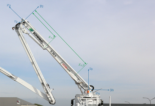
Here, the hydraulic cylinder is directly connected to the beam at $x_i=x_{c,2}$ and thus the elastic deformation is zero at this position, i.e. $v_2(x_{c,2})=0$. Additionally, the beam is connected to a rotational joint at the end $x_2=-l_2$, which results in the boundary conditions $v_2(-l_2)=0$ and $\left({\mathrm{\partial }}^2{v}_2/\mathrm{\partial }{x}_2^2\right)(x_2=-l_2)=0$ (zero torque). At the other end, the boundary equations are similar to (16), i.e.

(17a) ${\left.E_{y,2}{j}_{y,2}\left(x_2\right)\frac{{\mathrm{\partial }}^2{v}_2\left(x_2\right)}{\mathrm{\partial }{x}_2^2}\right|}_{x_2=0}=M_{z_2,0}$(17a)

(17b) ${\left.\frac{\mathrm{\partial }}{\mathrm{\partial }{x}_2}\left(E_{y,2}{j}_{y,2}\left(x_2\right)\frac{{\mathrm{\partial }}^2{v}_2\left(x_2\right)}{\mathrm{\partial }{x}_2^2}\right)\right|}_{x_2=0}=F_{y_2,0}.$(17b)

To calculate the stationary bending line, the beam element 2 is divided into two beam parts, each of which is modelled by (15). Using the boundary conditions together with the continuity requirement for $\left(\mathrm{\partial }{v}_2/\mathrm{\partial }{x}_2\right)$ and $\left({\mathrm{\partial }}^2{v}_2/\mathrm{\partial }{x}_2^2\right)$ at $x_{c,2}$ finally allows to numerically determine the stationary bending line of beam element 2.

The stationary bending in local $z$-direction, i. e. the horizontal direction, is similar to the bending in the vertical direction, except that (i) no gravitational term is present in (15) and, (ii) all link elements $i=2,\dots ,5$ have identical boundary conditions similar to (16). Since the resulting set of differential equations and boundary conditions is similar to the vertical direction, it is not detailed in this work.

The differential equations together with the corresponding boundary conditions for each link $2$ to $5$ are solved numerically in Matlab using the bvp4c solver. The resulting deformations are then approximated using the polynomials

(18a) ${\zeta }_{{\alpha }_i}=b_{{\alpha }_i}(l_i+x_i{)}^2+a_{{\alpha }_i}(l_i+x_i),i=2,3,4,5,$(18a)

(18b) ${\zeta }_{v_2}=b_{v_2}(x_2-x_{c,2})(l_2+x_2{)}^2+a_{v_2}(x_2-x_{c,2})(l_2+x_2),$(18b)

(18c) ${\zeta }_{v_i}=b_{v_i}(l_i+x_i{)}^3+a_{v_i}(l_i+x_i{)}^2,i=3,4,5,$(18c)

(18d) ${\zeta }_{w_i}=b_{w_i}(l_i+x_i{)}^3+a_{w_i}(l_i+x_i{)}^2,i=2,3,4,5.$(18d)

These polynomials are chosen to fulfil the geometric boundary conditions and the coefficients $a_{{\alpha }_i}$, $a_{v_i}$, $a_{w_i}$, $b_{{\alpha }_i}$, $b_{v_i}$, $b_{w_i}$, listed in Table 2, are calculated by a least-squares fit to the numerical solutions of the deformations. The results for the third beam element, shown in Figure 5, prove that a very accurate approximation of the stationary numerical solution is achieved by these polynomials. Similar results are obtained for all other beam elements.

Figure 5. Comparison of the normalized numerical solution of the static deformations ${\alpha }_3,v_3,w_3$ with the polynomial approximations ${\zeta }_{{\alpha }_3}$, ${\zeta }_{v_3}$, ${\zeta }_{w_3}$ for link 3.

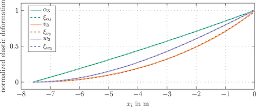
Table 2. Coefficients of the shape functions in (18).

link $i$	$a_{\alpha ,i}\cdot {10}^6$	$b_{\alpha ,i}\cdot {10}^6$	$a_{v,i}\cdot {10}^3$	$b_{v,i}\cdot {10}^6$	$a_{w,i}\cdot {10}^6$	$b_{w,i}\cdot {10}^6$
2	344.79	1.40	– 3.68	71.98	323.79	– 11.66
3	578.92	11.82	– 1.87	41.20	480.90	– 18.18
4	2386.40	– 55.70	– 2.10	90.20	1166.60	– 56.75
5	4729.30	1057.20	– 1.27	64.69	1260.80	– 29.93

Using the Ritz approximation (12), the system can be described by the overall set of generalized coordinates ${\mathbf{q}}^{\mathrm{T}}=[{\mathbf{q}}_r^{\mathrm{T}},{\mathbf{q}}_e^{\mathrm{T}}]\in {\mathbb{R}}^{17}$, with the rigid body joint angles ${\mathbf{q}}_r^{\mathrm{T}}=[q_1,\dots ,q_5]$ and the elastic degrees of freedom ${\mathbf{q}}_e^{\mathrm{T}}=[q_{{\alpha }_2},q_{v_2},q_{w_2},q_{{\alpha }_3},\dots ,q_{w_5}]$.

2.3. Dynamic model

The equations of motion of the boom are derived in this section by means of the Euler-Lagrange formalism utilizing the kinematics and the Ritz approximation described in the previous sections. First, the overall kinetic and potential energy are derived.

The first part of the kinetic energy is given by the kinetic energy of the elastic links. As described before, the elastic links are characterized by the line mass densities ${m_i}^{\prime }\left(x_i\right)$. To capture the kinetic energy due to the torsion of the links, the line inertia density ${{\Theta }^{\prime }}_i\left(x_i\right)$ around the local $x_i$-axis is utilized. This gives the overall kinetic energy $T_{l,i}$ of link $i$ in the form

(19) $T_{l,i}=\frac{1}{2}\underset{-l_i}{\overset{0}{\int }}{m^{\prime }}_i\left(x_i\right){\dot{\mathbf{p}}}_i^0{\left(x_i\right)}^{\mathrm{T}}{\dot{\mathbf{p}}}_i^0\left(x_i\right)+{\omega }_i^0{\left(x_i\right)}^{\mathrm{T}}{{\Theta }^{\prime }}_i^0\left(x_i\right){\omega }_i^0\left(x_i\right)\mathrm{d}{x}_i\hspace{0.17em}.$(19)

As described at the beginning of this section, joint 2 and 3 are actuated by linear hydraulic cylinders, whereas joint 4 and 5 are actuated by rotational hydraulic actuators. These actuators add a significant mass to the boom and thus have to be taken into account in the calculation of the overall kinetic energy. The rotational actuators are approximated by point masses $m_{a,i}$ placed in the corresponding joint, i.e. at the end of the link $i-1$. The mass of the linear cylinders is approximated by two point masses. The first point mass $m_{a,i}$ is attributed to the joint and the second one $m_{c,j}$ is added to the second link at the mounting point $x_{c,i}$ of the cylinder, see Figure 4. This gives the second part of the kinetic energy in the form

(20) $T_a=\frac{1}{2}\sum _{i=3}^5{m}_{a,i}{\dot{\mathbf{p}}}_{i-1}^0{\left(0\right)}^{\mathrm{T}}{\dot{\mathbf{p}}}_{i-1}^0\left(0\right)+\frac{1}{2}\sum _{i=2}^3{m}_{c,i}{\dot{\mathbf{p}}}_2^0{\left(x_{c,i}\right)}^{\mathrm{T}}{\dot{\mathbf{p}}}_2^0\left(x_{c,i}\right).$(20)

The overall kinetic energy of the boom reads as $T={\sum }_{i=2}^5{T}_{l,i}+T_a$.

The potential energy $V_g$ due to gravity is defined in a similar form by $V_g={\sum }_{i=2}^5{V}_{gl,i}+V_{ga}$. Here, the potential energy of the links $V_{gl,i}$ is given by

(21) $V_{gl,i}=-{\int }_{-l_i}^{0}m{{ }^{\mathrm{\prime }}}_i\left(x_i\right){\mathbf{g}}^{\mathrm{T}}{\mathbf{p}}_i^0\left(x_i\right)\mathrm{d}{x}_i,$(21)

with the vector of gravitational acceleration ${\mathbf{g}}^{\mathrm{T}}=[0,0,-g]$. The potential energy due to the actuators $V_{ga}$ reads as

(22) $V_{ga}=-\sum _{i=3}^5{m}_{p,i}{\mathbf{g}}^{\mathrm{T}}{\mathbf{p}}_{i-1}^0\left(0\right)-\sum _{i=2}^3{m}_{c,i}{\mathbf{g}}^{\mathrm{T}}{\mathbf{p}}_2^0\left(x_{c,i}\right).$(22)

The second part of the potential energy results from the elastic deformation of the links. Applying again the assumption of Saint-Venant and Bernoulli-Euler, the internal elastic (potential) energy $V_e$ reads as $V_e={\sum }_{i=2}^5(V_{e\alpha ,i}+V_{ev,i}+V_{ew,i})$, with

(23a) $V_{e\alpha ,i}=\frac{1}{2}{\int }_{-l_i}^0{G}_i{j}_{t,i}\left(x_i\right)\left(\frac{\mathrm{\partial }{\alpha }_i\left(x_i\right)}{\mathrm{\partial }{x}_i}\right)\mathrm{d}{x}_i$(23a)

(23b) $V_{ev,i}=\frac{1}{2}{\int }_{-l_i}^0{E}_{y,i}{j}_{y,i}\left(x_i\right){\left(\frac{{\mathrm{\partial }}^2{v}_i\left(x_i\right)}{\mathrm{\partial }{x}_i^2}\right)}^2\mathrm{d}{x}_i$(23b)

(23c) $V_{ew,i}=\frac{1}{2}{\int }_{-l_i}^0{E}_{z,i}{j}_{z,i}\left(x_i\right){\left(\frac{{\mathrm{\partial }}^2{w}_i\left(x_i\right)}{\mathrm{\partial }{x}_i^2}\right)}^2\mathrm{d}{x}_i.$(23c)

Here, $G_i,E_{y,i},E_{z,i}$ are the shear and Young’s modulus, $j_{t,i}$ is the torsional stiffness and $j_{y,i},j_{z,i}$ are the second moments of area.

To approximately account for the dissipative effects in the boom, viscous friction is modelled in the joints and a dissipation proportional to the rate of change is considered for the elastic degrees of freedom. This yields the Rayleigh dissipation function

(24) $R=\sum _{i=1}^5\frac{1}{2}{d}_{j,i}{\dot{q}}_i^2+\sum _{i=2}^5\frac{1}{2}{\int }_{-l_i}^0{d}_{t,i}{\dot{\alpha }}_i{\left(x_i\right)}^2+d_{v,i}{\dot{v}}_i{\left(x_i\right)}^2+d_{w,i}{\dot{w}}_i{\left(x_i\right)}^2\mathrm{d}{x}_i.$(24)

Although this is only a rough approximation of the real friction behaviour of the boom, it will be shown in the experimental validation of the model that a high accuracy can be achieved for the resulting dynamic behaviour.

The equations of motion are obtained by applying the Euler-Lagrange formalism, see, e.g. [13]

(25) $\mathbf{D}\left(\mathbf{q}\right)\ddot{\mathbf{q}}+{\tau }_C\left(\mathbf{q},\dot{\mathbf{q}}\right)+{\tau }_p\left(\mathbf{q}\right)+{\tau }_r\left(\dot{\mathbf{q}}\right)+{\tau }_d\left(\mathbf{q},{\mathbf{f}}_d\right)=\tau .$(25)

The generalized mass matrix $\mathbf{D}$ is calculated by

(26) $\mathbf{D}=\frac{\mathrm{\partial }}{\mathrm{\partial }\dot{\mathbf{q}}}{\left(\frac{\mathrm{\partial }}{\mathrm{\partial }\dot{\mathbf{q}}}T\right)}^{\mathrm{T}},$(26)

the vector of Coriolis forces reads as

(27) ${\tau }_C=\dot{\mathrm{D}}\dot{\mathrm{q}}-\frac{1}{2}{\dot{q}}^{\mathrm{T}}\frac{\mathrm{\partial }\mathbf{D}}{\mathrm{\partial }\mathbf{q}}\dot{q},$(27)

and the vector of potential forces ${\tau }_p$ is given by ${\tau }_p=\mathrm{\partial }\left(V_g+V_e\right)/\mathrm{\partial }\mathbf{q}$. The dissipation is represented by ${\tau }_r=\mathrm{\partial }R/\mathrm{\partial }\dot{q}$ and the actuators are described by the generalized forces $\tau =[{\tau }_1,\dots ,{\tau }_5,0_{1\times 12}{]}^{\mathrm{T}}$. Finally, an additional disturbance force ${\mathbf{f}}_d$ is assumed to act on the end effector at the position ${\mathbf{p}}_5^0$, which is equivalently taken into account by the generalized force ${\tau }_d$, see, e.g. [13]

(28) ${\tau }_d^{\mathrm{T}}={\mathbf{f}}_d^{\mathrm{T}}\frac{\mathrm{\partial }}{\mathrm{\partial }\mathbf{q}}{\mathbf{p}}_5^0\hspace{0.17em}.$(28)

This disturbance force is used to approximately consider disturbances resulting, e. g, from the pumping of concrete. Furthermore, it is used in the validation experiments, where an external load is connected to the end of the boom.

2.4. Model simplifications

Since the mathematical model is intended to serve as a basis for the controller design, in the following, measures to reduce the computational costs will be presented.

First, the detailed construction of the links, which includes inhomogeneous stiffness and offsets, is approximated by links with box sections and linearly varying mass and inertia along the local axis $x_i$, see Figure 6 for this simplified geometry. The mass distribution is formulated as ${m_i}^{\prime }\left(x_i\right)=m{{ }^{\mathrm{\prime }}}_{i,1}+\left({m{ }^{\mathrm{\prime }}}_{i,1}-{m{ }^{\mathrm{\prime }}}_{i,0}\right)x_i/l_i$, where $m{{ }^{\mathrm{\prime }}}_{i,0}$ and $m{{ }^{\mathrm{\prime }}}_{i,1}$ represent the line mass densities at the beginning $x_i=-l_i$ and the end $x_i=0$ of the link, respectively. The moment of inertia ${\mathrm{\Theta }}_{xx,i}$ around the local $x_i$-axis is defined similarly in the form ${{\mathrm{\Theta }}_{xx,i}}^{\prime }\left(x_i\right)=\mathrm{\Theta }{{ }^{\mathrm{\prime }}}_{xx,i,1}+\left({\mathrm{\Theta }{ }^{\mathrm{\prime }}}_{xx,i,1}-{\mathrm{\Theta }{ }^{\mathrm{\prime }}}_{xx,i,0}\right)x_i/l_i$, with

Figure 6. Sketch of the simplified beam geometry for link 4 (cross-section and top view).

(29a) $\mathrm{\Theta }{{ }^{\mathrm{\prime }}}_{xx,i,0}=\rho {\int }_{A_i\left(-l_i\right)}{y}_i^2+z_i^2\hspace{0.17em}\mathrm{d}{A}_i$(29a)

(29b) $\mathrm{\Theta }{{ }^{\mathrm{\prime }}}_{xx,i,1}=\rho {\int }_{A_i\left(0\right)}{y}_i^2+z_i^2\hspace{0.17em}\mathrm{d}{A}_i$(29b)

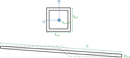
Therein, $A_i(x_i)$ is the position-dependent cross-sectional area of the link and $\rho$ is the mass density. In accordance with the Euler-Bernoulli assumptions, the moments of inertia around the local $y_i$- and $z_i$-axis are neglected. Therefore, the matrix of inertia density is given by ${\mathbf{\Theta }{ }^{\mathrm{\prime }}}_i=\mathrm{d}\mathrm{i}\mathrm{a}\mathrm{g}[\mathrm{\Theta }{{ }^{\mathrm{\prime }}}_i,0,0]$.

The torsional stiffness $j_{t,i}$ along the beam is also approximated by a linear function

(30) $j_{t,i}\left(x_i\right)=j_{t,i,1}+\left(j_{t,i,1}-j_{t,i,0}\right)\frac{x_i}{l_i},$(30)

where $j_{t,i,0}$ and $j_{t,i,1}$ represent the torsional stiffness at the beginning and end of each link $i$. They are calculated using the empirical formula, see, e.g. [19]

(31) $j_{t,i}(x_i)=\frac{2b_{w,i}{(x_i)}^2{(b_{y,i}(x_i)-b_{w,i}(x_i))}^2{(b_{z,i}(x_i)-b_{w,i}(x_i))}^2}{b_{y,i}(x_i)b_{w,i}(x_i)-2b_{w,i}{(x_i)}^2+b_{z,i}(x_i)b_{w,i}(x_i)},$(31)

using $x_i=-l_i$ for $j_{t,i,0}$ and $x_i=0$ for $j_{t,i,1}$. The dimensions of the box section $b_{y,i}$, $b_{z,i}$, and $b_{w,i}$ are defined in Figure 6.

Since the elastic deformations do not significantly change the mass distribution of the beam elements, only the rigid body kinematics, i. e. ${\mathbf{q}}_e=\mathbf{0}$, are used for the transformation ${\mathbf{R}}_0^i$ of the inertia matrices ${{\Theta }^{\prime }}_i$ to the inertial frame ${{\Theta }^{\prime }}_i^0={\mathbf{R}}_0^i{{\Theta }^{\prime }}_i({\mathbf{R}}_0^i{)}^{\mathrm{T}}$, which is required for the kinetic energy in (19). Accordingly, the mass matrix $\mathbf{D}$ is evaluated for the undeformed configurations of the links $\mathbf{D}={\left.\mathbf{D}\right|}_{{\mathbf{q}}_e=\mathbf{0}}$. Due to the relatively slow motion of the boom, the influence of the computationally expensive Coriolis forces is marginal and thus neglected, i.e. ${\tau }_C=0$.

3. Model calibration

The mathematical model developed in the last section contains numerous parameters that have to be determined. Most of the parameters, as, e. g, the geometry, can be obtained from the construction data of the boom. There are, however, a number of other parameters, where only rough estimates are available:

1. The mass distribution $m{{ }^{\mathrm{\prime }}}_i\left(x_i\right)$ of the simplified beam elements is only an approximation of the real links’ mass distribution, since the construction is rather complex and an accurate representation would increase the model’s complexity significantly.

2. An accurate estimation of the stiffness of the beam elements from construction data is difficult, since the construction is rather complex and the attached elements also influence the overall stiffness.

3. As already discussed in Section 2.3, it is very difficult to estimate the friction and damping of the boom from construction data.

To achieve the desired accuracy of the mathematical model, these parameters will be identified by measurements. The main goal of the model calibration is to accurately represent (i) the stationary bending of the boom, in particular at the end effector, and (ii) to capture the dominating vibration frequencies of the system for various configurations.

3.1. Measurement setup

In order to calibrate and validate the proposed model, the machine is equipped with a number of sensors:

• At each of the five joints, a joint angle sensor is attached. These industrial standard joint angle sensors are designed for robust operation under harsh conditions. This limits their measurement accuracy to the range of $1^{\circ }$. Additionally, a nonlinearity over the whole measurement range can be observed. Thus, these sensors will only give coarse information of the boom configuration, which is sufficient for control purposes but not well suited for model calibration.

• Inertial measurement units (IMU) that measure both the three-dimensional accelerations and angular rates are attached to the end of each link.

These sensors do not allow for measurements of the absolute position of the elastic link elements. Therefore, an additional camera setup is used in combination with a computer vision algorithm. This enables a reconstruction of the 3D position of optical markers that are attached to the boom. The overall sensor concept for the calibration experiments is depicted in Figure 7.

Figure 7. Sensor setup used for the calibration experiments.

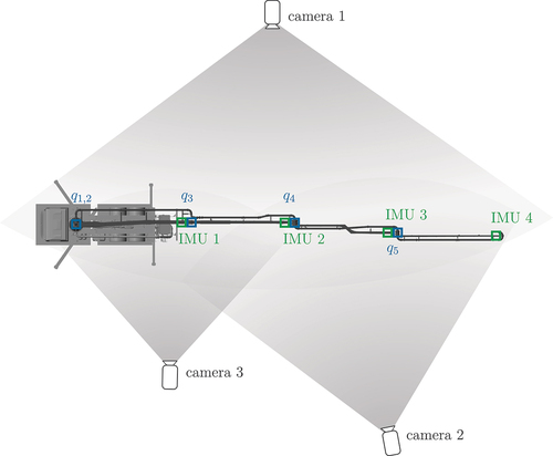
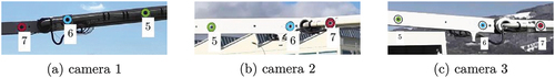
Since the camera-based position measurement is a central element in the model calibration, the main ideas and steps of these measurements are briefly summarized. In Figure 7, the positions of the three cameras including their field of view are shown. Camera 1 is placed on one side of the machine, capturing the whole area of interest. Placing cameras on both sides of the machine is beneficial concerning the measurement accuracy in the horizontal plane. This, however, requires to mount fiducial markers on both sides of the boom, which will be addressed in detail later. On the opposite side, two cameras were placed, where camera 2 also captures the whole boom but is positioned closer to the end of the boom. The field of view of camera 3 only covers the first two boom elements in the configuration depicted in Figure 7. This is meaningful, since the elastic deflections of the first two links are significantly smaller than the elastic deflections of the third and fourth link. Placing camera 3 close to link 1 and 2 allows for a higher resolution for the position measurements of these links.

On each link, three fiducial markers are attached to both sides of the boom, see Figure 8. The markers are chosen to have a high response to feature-based detection algorithms, see [20]. Additionally, a set of markers is attached to the carrier truck to serve as reference points. Using the Computer Vision toolbox in Matlab, the camera coordinates of the fiducial markers are detected by KAZE features, see, e.g. [21]. The motion of these markers is tracked using the marker tracking functions of the Computer Vision toolbox in Matlab. An example of the marker tracking for the three cameras is given in Figure 9.

Figure 8. The manipulator in the transport configuration with attached fiducial markers.

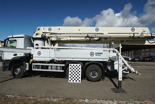
Figure 9. Example results of the KAZE marker tracking for the three cameras.

This procedure leads to time series of tracked image coordinates ${\mathbf{P}}_{j,k}$ for each fiducial marker $j$ and camera $k$. The image coordinates ${\mathbf{P}}_{j,k}$ are a projection of the 3-dimensional real-world position ${\mathbf{p}}_j$ of the marker $j$ to the considered camera frame given as³, see, e.g. [22]

(32) ${\mathbf{P}}_{j,k}={\mathcal{P}}_k{\mathbf{p}}_j,$(32)

where ${\mathcal{P}}_k$ is the so-called camera matrix of camera $k$. It is obtained by intrinsic calibration using a chequerboard and extrinsic calibration using known reference points of the machine. Thereby, the intrinsic calibration aims at minimizing the lens and sensor distortions by reducing the quadratic error between measured and known corner points of a standard black and white chequerboard, see, e. g. [23]. With the extrinsic calibration, the exact position and orientation of the camera frame w. r. t. the inertial coordinate frame ${\mathrm{\Sigma }}_0$ is found.

Given the image coordinates ${\mathbf{P}}_{j,k}$ of two or three cameras (depending on the position of the marker on the boom and the field of view of the cameras), it is now possible to reconstruct the real-world 3D position of the point ${\mathbf{p}}_j$. Since camera 1 sees the opposite side of the boom compared to camera 2 and 3, the cameras do not see the same markers, see Figure 7. To account for this fact, the position of the two markers seen by the cameras at the opposite side of the boom are calculated by ${\mathbf{p}}_{j,k}={\mathbf{p}}_j-{\mathbf{p}}_{j,k}^{\mathrm{o}\mathrm{f}\mathrm{f}}$, where ${\mathbf{p}}_j$ is the position of a virtual marker and ${\mathbf{p}}_{j,k}^{\mathrm{o}\mathrm{f}\mathrm{f}}$ describes the known constant offset of the marker $j$ in the field of view of camera $k$. In this way, markers which are located at the same position $x_i$ at each boom element but on opposite sides are merged to a single one. The back-projection of the marker positions in the camera image to the three-dimensional real world is then formulated as the optimization problem

(33) $\underset{{\mathbf{p}}_j\in {\mathbb{R}}^3}{min}\sum _{k=1}^{N_{cam}}∥{\mathbf{P}}_{j,k}-{\mathcal{P}}_k\left({\mathbf{p}}_j-{\mathbf{p}}_{j,k}^{\mathrm{o}\mathrm{f}\mathrm{f}}\right)∥,$(33)

where $N_{cam}$ is the number of camera images available for the current marker $j$ (either 2 or 3 in this work).

3.2. Calibration process

The focus of the model calibration is to achieve a high accuracy for the simulation of the dominating elastic effects of the large-scale manipulator. In the first step of the model calibration, the line mass densities $m{{ }^{\mathrm{\prime }}}_i\left(x_i\right)$ are adjusted such that the total link mass

(34) $m_i={\int }_{-l_i}^{0}m{{ }^{\mathrm{\prime }}}_i\left(x_i\right)\mathrm{d}{x}_i$(34)

as well as the centre of gravity along the neutral line

(35) $x_{cog,i}=\frac{1}{m_i}{\int }_{-l_i}^0{x}_{i}m{{ }^{\mathrm{\prime }}}_i\left(x_i\right)\mathrm{d}{x}_i$(35)

match the actual link mass and centre of gravity measured by the industrial partner. This mass $m_i$ includes the mass of all attached additional components, as e.g. the concrete and hydraulic pipes. The point masses $m_{a,i}$, $m_{c,i}$, which describe the actuator masses, are accurately known from construction data and thus remain unchanged.

In the next step, the parameters describing the elasticity of the links, i. e, the Young’s modulus $E_{y,i}$, $E_{z,i}$ and the shear modulus $G_i$, are manually tuned to match the deflections and the dominating vibration frequencies of the boom. To do so, the following experiments are performed:

• The stationary elastic deformations are measured by applying a load force ${\mathbf{f}}_d$ to the end of the boom at the origin of ${\mathrm{\Sigma }}_5$. This load force is generated by a load mass of $m_d=100\mathrm{k}\mathrm{g}$, which is connected to the boom by means of a rope. Utilizing a pulley, the load force ${\mathbf{f}}_d$ can be applied in vertical $z_0$- and horizontal $y_0$-direction. Due to the connection by means of a rope, no torques are introduced at the end of the boom.

• After loading the boom with the mass and measuring the stationary deflection, the rope is cut. This releases the load mass from the boom and results in a rapid motion of the boom. From these experiments, the dynamic response of the boom, in particular the dominating vibration frequency and amplitude, are obtained.

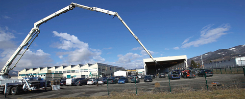
These experiments are repeated for different load directions and two configurations of the boom. The stretched configuration depicted in Figure 10 is the configuration with the largest overall deflections, and thus of particular interest for the model calibration. For a visual reference, Figure 10 shows the deflections both for the case with and without the load mass attached to the boom. The bow-like configuration shown in Figure 11 is typical for the operation of the mobile concrete pump and thus of high practical relevance.

Figure 10. Stretched configuration of the boom: the loaded ($100$ kg at the boom’s end) and unloaded configuration are merged in this figure.

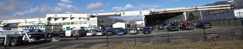
Figure 11. Bow-like configuration used in the calibration experiments.

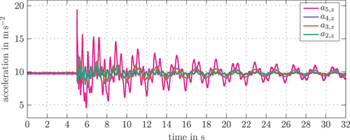
Since the measurement of the joint angles is rather inaccurate, it is not meaningful to aim for a high accuracy of the absolute positions of the calibrated model. Instead, the model calibration is performed in a way that the relative differences of the fiducial markers of the boom with and without load is achieved. For the calibration of the dynamic vibrations of the system, additionally the acceleration sensors of the IMUs are utilized. Figure 12 shows the measured accelerations of an experiment right after the load was separated from the boom. It can be observed that, as expected, the sensor placed at the end of link 2 measures comparatively low accelerations $a_{2,z}$, while the acceleration $a_{5,z}$ at the end of link 5 shows significantly larger amplitudes. Moreover, it is visible that there is one dominant vibration frequency after the high-frequency harmonics decayed.

Figure 12. Acceleration measurements of the IMU after separation of the load for the stretched configuration.

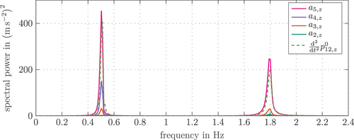
This becomes even more obvious when applying the fast Fourier transformation (FFT) to the measured accelerations. The results in Figure 13 show a first maximum around $0.5$ Hz. The second peak around $1.8$ Hz exhibits a significantly smaller amplitude. To validate these measurement results, also the FFT of the time series of the acceleration in the $z_0$-axis of the last fiducial marker $\frac{{\mathrm{d}}^2}{\mathrm{d}{t}^2}{p}_{12,z}^0$ at the end of link 5 is calculated. Clearly, they show the same vibration frequencies. In the following, the model calibration is focused on the first dominant frequency of the boom, since it is also related to the largest amplitudes.

Figure 13. FFT of the measured IMU accelerations and the acceleration of the last fiducial marker $\frac{{\mathrm{d}}^2}{\mathrm{d}{t}^2}{p}_{12,z}^0$ obtained by the computer vision system for the stretched boom.

Four experiments were performed for the calibration of the vertical elasticity, and three experiments for the horizontal elasticity. For the tuning of the elasticities, these measurements are compared to the equivalent model outputs that are obtained by solving the equations of motion numerically in Matlab/Simulink 2021b (solver ode23t), where the rigid body angles ${\mathbf{q}}_r$ obtained by the joint angle sensors serve as model input. Using the manipulator’s kinematic equations, e.g. for an optical marker attached to link 5, the simulated 3D position of the marker is obtained by

(36) ${\hat{\mathbf{p}}}_j^0={\mathbf{H}}_5^0\left(\mathbf{q}\right){\hat{\mathbf{p}}}_j,$(36)

where ${\mathbf{p}}_j$ is the constant position of the marker $j$ given in the local frame ${\mathrm{\Sigma }}_5$. After calibrating the elasticity of the boom, the damping coefficients are manually tuned in the final step to match the decay times of the measured vibrations.

3.3. Results

In this section, the model is validated by comparison of the calibrated model with measurements. For this evaluation, the stationary deflections are measured for two different configurations and loading directions of the boom, see Table 3 for a detailed description of these experiments. The scalar $\mathrm{\Delta }{p}_{12}^0$ denotes the step difference of the last fiducial marker $j=12$, in the negative direction of the external force ${\mathbf{f}}_d$. The results of the stationary differences are depicted in Figure 14 and summarized in Table 3. These stationary measurements prove that the calibrated model has a high accuracy, with maximum errors in the range of $15\mathrm{\%}$. It has to be noted that due to limited resolution of the vision-based measurement system in the horizontal plane as well as neglected effects like stiction friction similar experimental setups lead to slightly different absolute positions, as can be seen in experiment 2 and 3 as well as in experiment 5 and 6. Compared to the workspace of the manipulator of 36 m, these errors are small and the calibration aims for the best compromise for all experiments. Due to the huge effort to obtain measurements on the real system, only a small number of measurements was made available for this work.

Figure 14. Model validation: Stationary differences for the displacements of marker 12 mounted at the end of the boom for the loaded and unloaded manipulator.

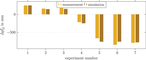
Table 3. Results for the stationary differences. Comparison of the displacements of marker 12 mounted at the end of the boom for the unloaded and loaded manipulator.

number	configuration	${\mathbf{f}}_d$ direction	$\mathrm{\Delta }{p}_{12,meas}^0$	$\mathrm{\Delta }{p}_{12,sim}^0$	error in
			in mm		w. r. t. $\mathrm{\Delta }{p}_{12,meas}^0$
1	stretched	$-z_0$	245	245	$0.10$
2	bow	$-z_0$	158	143	$-9.24$
3	bow	$-z_0$	176	150	$-14.61$
4	stretched	$+z_0$	$-216$	$-246$	$14.16$
5	stretched	$+y_0$	$-660$	$-756$	$14.35$
6	stretched	$+y_0$	$-840$	$-755$	$-10.15$
7	bow	$+y_0$	$-788$	$-773$	$-1.92$

To compare the simulated dynamics with the measurements, the FFT of the signals around the first dominant frequency is given for experiment 1 in Figure 15. The normalized power of the measured accelerations show a similar result for the model and the measurement. The small offset in the frequency is assumed to result from the model simplifications, which, however, is not of much relevance for the application of the model in the dynamic simulation. Furthermore, these inaccuracies can be well handled by a damping control strategy as published, e. g, in [14]. The results for the other experiments are summarized in Table 4 and Figure 16. Here, an additional experiment denoted as T-shaped configuration is added, where the manipulator is in an upright T-shaped configuration. In this configuration, a short step-like torque is applied to the first joint of the boom, which results in a rotation around the global $z$-axis. With this experiment, the impact of the torsional deformation of the boom is validated. The results for calibration experiment 1 and 6 are presented in Figure 17 as time series, showing the simulation output of the model before the calibration process as well.

Figure 15. Model validation: FFT of the simulated and measured acceleration for experiment 1.

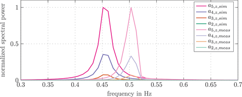
Figure 16. Model validation: Results of the first vibration frequency at the end of the boom.

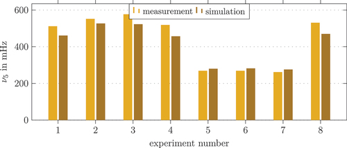
Figure 17. Comparison of the relative deflection of marker 12 placed at the end effector for the measured (computer vision) and the calibrated and uncalibrated simulation model.

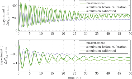
Table 4. Results of the dynamic calibration: ${\nu }_5$ is the first vibration frequency at the end of the boom (measured by IMU 5).

number	configuration	${\mathbf{f}}_d$ direction	${\nu }_{5,meas}$	${\nu }_{5,sim}$	error in
			in mm		w. r. t. ${\nu }_{5,meas}$
1	stretched	$-z_0$	512	461	$-9.96$
2	bow	$-z_0$	552	527	$-4.53$
3	bow	$-z_0$	577	523	$-9.36$
4	stretched	$+z_0$	$519$	$457$	$-11.95$
5	stretched	$+y_0$	$269$	$280$	$4.09$
6	stretched	$+y_0$	$269$	$282$	$4.83$
7	bow	$+y_0$	$262$	$276$	$5.34$
8	T-shaped	–	$531$	$470$	$-11.49$

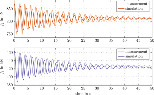
For further validation of the model, the cylinder forces of joint 2 and 3, denoted by $f_2$ and $f_3$, are investigated in Figure 18 for experiment 1. This validation is of specific interest for the model-based controller design, since the actuator forces and torques will be limited in the real application and thus, an accurate representation in the model is important. The results in Figure 18 show a good agreement in the vibration amplitude and damping behaviour. The comparably small errors between the simulated and measured forces result from the aforementioned model simplifications. For the actuators in joint 4 and 5, no torque measurement is available, and thus no comparison is possible.

Figure 18. Model validation: actuator forces of the cylinders for joints 2 and 3 for experiment 1.

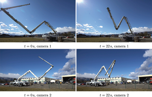
The experiments utilized for the model validation so far are rather academic test cases that will not occur in real operation of the mobile concrete pump. In particular, it is rather unusual that a large step-like change in the load at the end effector will occur. Thus, the final validation of the calibrated model is based on a more realistic scenario. In this scenario, the boom is manually steered by the operator via a handheld remote control from a configuration, shown in Figure 21 on the left, to the transport configuration (see Figure 8). Using the measurements of the joint angles, the same scenario is simulated with the calibrated model. This scenario also comprises strong excitations of elastic vibrations and is therefore very challenging for numerical simulation. The simulation on a standard PC (Intel i7-6700 K®, 16 GB, Ubuntu 18.04.6) takes 93 s for the whole measurement of 300 s, which proves the low computational costs of the proposed model. The simulated and measured Cartesian position of the end effector are shown in Figure 19 and the joint angles are depicted in Figure 20. At $t=22$ s, the end effector marker as seen from camera 1 is covered by the other links as shown in Figure 21 on the right, which results in an increase of the position error to an almost constant offset after approximately 55 s, see Figure 19. Still, during the time span between $t=0$ s and $t=50$ s where most of the end effector motion is happening, the position error $\mathrm{\Delta }{\mathbf{p}}_{12}$ stays within acceptable limits and the movement is represented correctly. Although the first joint (the slewing gear) is not rotated during this experiment, there is a small motion of the end effector in the $y$-direction, which results from the offsets of the links in combination with the elastic deformation $w_i$ and torsion ${\alpha }_i$ of the boom.

Figure 19. Simulated and measured position of marker 12 placed at the end effector during the fold-in scenario.

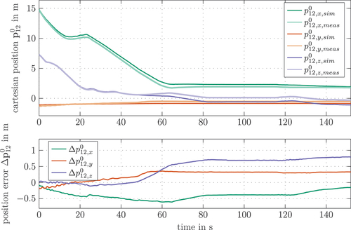
Figure 20. Generalized coordinates $\mathbf{q}$ of the simulation model for the fold-in scenario.

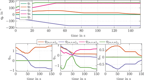
Figure 21. Camera measurement snapshots showing the start configuration at $t=0$ and the covering of the end effector for camera 1 after $t=22$.

Figure 20 also shows the simulated elastic degrees of freedom $q_{{\alpha }_i}$, $q_{v_i}$ and $q_{w_i}$ for this scenario. Taking a look at link 2, it can be seen that its torsion $q_{{\alpha }_2}$ and bending $q_{w_2}$ are of the same sign and similar scale at the beginning and end of the motion. This is meaningful, since the orientation of link 2 is also almost identical in the start and transport configuration. In contrast, the bending $q_{v_2}$ decreases, which is due to the reduced load by the links attached to link 2 in the transport configuration compared to the start configuration. A similar result is given for link 3, however, here the torsion $q_{{\alpha }_3}$ and bending $q_{w_3}$ change sign during the fold-in. This results from the fact that link 3 is pointing in the opposite direction in the start and transport configuration. The elastic deformations of link 4 and 5 due to torsion $q_{{\alpha }_i}$ and bending $q_{w_i}$ are very small, which is due to the fact that almost no offset is given for the corresponding links. Again, the bending $q_{v_5}$ shows the same sign and similar scale at the beginning and end of the motion due to the very similar orientation at those instances of time.

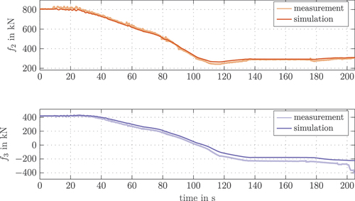
The forces of the actuators of joint 2 and 3 are depicted in Figure 22. The measured and simulated values are in good agreement, where the small errors arise from the model simplifications and an idealized model of the actuator dynamics, without considering the hydraulic circuit. The simulation in Figure 22 shows the forces calculated from the simulated generalized forces $\tau$ according to (25) and the kinematics of the joint mechanisms depicted in Figure 4. It proves that the idealized actuator model is a valid approximation.

Figure 22. Forces of the joints 2 and 3 during the fold-in scenario.

4. Conclusions

This work presented a mathematical model for the boom of a mobile concrete pump, which comprises five individual rotational joints and four lightweight links. The proposed mathematical model is based on first-principles modelling and allows to be executed with low computational effort. Furthermore, a computer vision based calibration of the model was developed. Specific experiments with step-like excitation demonstrated that the model parameters could be tuned in such a way that a high stationary accuracy as well as an accurate representation of the first dominant vibration frequency of the system for different boom configurations and excitation directions can be achieved. The resulting calibrated model was validated using a typical fold-in motion of the boom. Current research of the authors is directed towards the usage of this model in the design of optimal path planning and control strategies for the boom.

Acknowledgments

The authors further acknowledge TU Wien Bibliothek for financial support through its Open Access Funding Programme.

Disclosure statement

No potential conflict of interest was reported by the author(s).

Additional information

Funding

This work was supported by the Österreichische Forschungsförderungsgesellschaft [866 065].

Notes

1. Lightweight construction of the boom for enabling large workspace dates back to the very beginning of mobile concrete pump developments in the 1960s, see, e. g https://schwing-stetter.com/en/company/milestones.html or https://www.putzmeister.com/web/northamerica/history.

2. It has to be noted that although the choice of the shape function is based on the static deformation of the boom, the resulting model also exhibits a good accuracy for the dynamic case, as it will be shown by measurement results in Section 3.3.

3. In order to keep the notation short, the intrinsic normalization step is not explicitly formulated in this mapping.

References

- W.L. Hallauer and R.Y.L. Liu, Beam bending-torsion dynamic stiffness method for calculation of exact vibration modes, J. Sound Vib. 85 (1982) (1982), pp. 105–113. doi:10.1016/0022-460X(82)90473-4.
- O. Bruls, Integrated Simulation and Reduced-Order Modeling of Controlled Flexible Multibody Systems, Ph.D. diss, Université de Liège, Belgium, 2005.
- S.K. Dwivedy and P. Eberhard, Dynamic analysis of flexible manipulators, a literature review, Mech Machine Theor 41 (2006), pp. 749–777. doi:10.1016/j.mechmachtheory.2006.01.014.
- H. Bremer, Elastic Multibody Dynamics: A Direct Ritz Approach, SpringerDordrecht, Netherlands, 2008. doi:10.1007/978-1-4020-8680-9.
- M. Hiller, Modelling, simulation and control design for large and heavy manipulators, Rob Auton Syst 19 (2) (1996), pp. 167–177. doi:10.1016/S0921-8890(96)00044-9.
- J. Henikl, W. Kemmetmüller, M. Bader, and A. Kugi, Modelling, simulation and identification of a mobile concrete pump, Math Comput Model Dyn Syst 21 (2) (2015), pp. 180–201. doi:10.1080/13873954.2014.926277.
- J. Henikl, Regelungsstrategien für den Ausleger einer Autobetonpumpe, Shaker , Aachen, Germany, 2016. ISBN:978-3-8440-4541-3.
- S. Zorn, Modellbasierte aktive Schwingungstilgung eines Multilink-Groß raummanipulators, Ph.D. diss, Technische Universität Dresden, Dresden, Germany, 2017.
- J. Wanner and O. Sawodny, A lumped parameter model of the boom of a mobile concrete pump, in Proceedings of the 18th European Control Conference (ECC), Naples, Italy. 2019, Jun, 25-28, pp. 2808–2813. doi:10.23919/ECC.2019.8796004.
- E. Wittbrodt, I. Adamiec-Wójcik, and S. Wojciech, Dynamics of Flexible Multibody Systems: Rigid Finite Element Method, Heidelberg, Germany, Springer, Berlin, 2007. doi:10.1007/978-3-540-32352-5.
- S. Moberg, Modeling and Control of Flexible Manipulators, Ph.D. diss, Linköping University, Linköping, Sweden, 2010.
- A. Pertsch and O. Sawodny, Modelling and control of coupled bending and torsional vibrations of an articulated aerial ladder, Mechatronics 33 (2016), pp. 34–48. doi:10.1016/j.mechatronics.2015.11.009.
- B. Siciliano and O. Khatib (eds.), Springer Handbook of Robotics, Springer , Berlin, Heidelberg, Germany, 2008. doi:10.1007/978-3-540-30301-5.
- J. Henikl, W. Kemmetmüller, T. Meurer, and A. Kugi, Infinite-dimensional Decentralized Damping Control of Large-scale Manipulators with Hydraulic Actuation, Automatica 63 (2016), pp. 101–115. doi:10.1016/j.automatica.2015.10.024.
- A.A. Shabana, Dynamics of Multibody Systems, Cambridge University Press, Cambridge, 2013. doi:10.1017/CBO9781107337213.
- M.W. Spong, S. Hutchinson, and M. Vidyasagar, Robot Modeling and Control, John Wiley & Sons , New York, USA, 2006. ISBN:978-1-119-52399-4.
- M. Gander and G. Wanner, From Euler, Ritz, and Galerkin to Modern Computing, SIAM Review 54 (4) (2012), pp. 627–666. doi:10.1137/100804036.
- C. Unger, Optimale Trajektorienplanung für Manipulatoren mit elastischen Elementen, Master’s thesis, TU Wien, 2020. doi:10.34726/hss.2020.57984
- W.C. Young, R.G. Budynas, and A.M. Sadegh, Roark’s Formulas for Stress and Strain, Eighth Edition, McGraw-Hill , New York, USA, 2012. ISBN:978-0071742474.
- F. Schweiger, B. Zeisl, P. Georgel, G. Schroth, E. Steinbach, and N. Navab, Maximum Detector Response Markers for SIFT and SURF, in Proceedings of the 14th International Workshop on Vision, Modeling, and Visualization, Braunschweig, Germany, 2009 Nov (16-18), pp. 145–154. ISBN:978-3-9804874-8-1.
- P.F. Alcantarilla, A. Bartoli, and A.J. Davison, KAZE Features, in Proceedings of the 12th European Conference on Computer Vision, Florence, Italy. 2012, Oct, 7-13, pp. 214–227. doi:10.1007/978-3-642-33783-3_16.
- R. Hartley and A. Zisserman, Multiple View Geometry in Computer Vision, Cambridge University Press, Cambridge, UK, 2004. doi:10.1017/CBO9780511811685.
- P. Corke, Robotics, Vision and Control: Fundamental Algorithms in MATLAB, Springer doi:10.1007/978-3-642-20144-8, Cham, Germany, 2017.