Modeling and analysis of thin film flow of Fuzzified Johnson Segalman nanofluid using fuzzy extension of He-Laplace scheme

ABSTRACT

The concept of fuzzy calculus in fluid modelling offers a feasible approach to address ambiguity and uncertainty in physical phenomena. This study aims to model and analyse thin film flow of Johnson Segalman nonofluid (JSNF) on a vertical belt in fuzzy environment for lifting and drainage settings. By incorporating Triangular fuzzy numbers (TFNs), a more accurate representation of the uncertain nature of JSNF flow is obtained which leads to a better understanding of fluid behaviour and its potential applications. The fluid problems are modelled with uncertainties and numerically solved through fuzzy extension of He-Laplace algorithm. The validity and convergence of the proposed methodology is checked by computing residual errors in each case. The obtained solutions provide fuzzy velocity profiles and volumetric flow rates in lift and drain cases. As the parameter $r-cut$ approaches 1, the velocity profiles at the upper and lower bounds merge, indicating solution consistency.

KEYWORDS:

• Johnson Segalman modal
• Laplace transform
• Homotopy perturbation

Introduction

Fuzzy set theory (FST) was introduced by Zadeh [1] as a practical approach for handling uncertain data. FST utilizes membership functions for the assignment of values in domain and known as fuzzy numbers. These fuzzy numbers are represented by membership functions with a domain of zero to one, where each number is assigned a grade of membership. Authors have developed arithmetic operations for fuzzy numbers to address ambiguity [2]. The trapezoidal neutrosophic Dombi fuzzy hybrid operator is used by Fahmi in [3]. Rahaman et al. [4] studied linear fuzzy difference equation through Gaussian fuzzy number. The hesitant fuzzy arithmetic is examined by Ranjbar et al. in [5]. Recently, Tansel et al. [6] utilized triangular fuzzy numbers to develop a new and optimized machine performance. Moreover, Jena et al. [7] used Gaussian fuzzy numbers to examine geometrical uncertainties of Euler-Bernoulli beams.

Real-world problems are often ambiguous and challenging to address. Researchers have traditionally relied on differential equations for modelling and simulation of different problems. However, the data collected for modelling a phenomena are often inadequate in capturing uncertainties. Consequently, the resulting differential equations fail to accurately capture the scenario. To overcome this limitation, fuzzy differential equations (FDEs) are modelled for such situations. FDEs provide a framework for handling and incorporating uncertainty into the modelling process. Seikala [8] pioneered the concept of fuzzy differentiability. Later on, fuzzy integrability and differentiability was extended by Kaleva [9]. Fuzzy differential equations were firstly addressed by Kandel and Byatt [10] using extension principle and Fuzzy numbers. In [11], Nieto and Juan demonstrated the uniqueness and existence of Cauchy problem for FDEs. Prakash et al. [12] analysed two-point fuzzy BVPs using differential transform technique. Marzieh [13] investigated fuzzy linear DEs under granular differentiability. Khastan et al. uses generalized differentiability concept to second order fuzzy BVPs in [14]. Khan et al. [15] conducted research on selection of renewable energy sources using generalized fuzzy soft sets. Qayyum et al. proposed new solutions of fuzzy-fractional Fisher models in [16,17].

Fluid flow phenomena is extremely important in science and engineering [18–20]. A wide variety of problems, including heat and mass transfer [21], magnetic and porosity effects [22] are on the rise. These problems ultimately convert into differential equations that may contain uncertainty or noise. In general, different physical parameters and conditions of problems have major impact on differential equations. Such parameters and conditions are not crisp (certain) in most of the physical situations in reality due to experimental, mechanical and measurement defaults. FST is therefore a more appropriate approach than assuming crisp situation for better understanding and prediction. To make it more explicit, FDEs are essential in explaining noise/inaccuracy and providing a suitable framework for describing real world phenomena. Recently, researchers have started working on fuzzy fluid problems. Nadeem et al. investigated third-grade fuzzy hybrid nanofluid between two plates in [23]. Nadeem et al. also investigated fuzzy third grade fluid in inclined channel using triangular fuzzy numbers (TFNs) in [24]. Siddique et al. [25] also explored fuzzy thin film of third grade fluid. Nadeem et al. [26] investigated fully developed plane Poiseuille flow and the plane Couette-Poiseuille flow of a third-grade non-Newtonian fluid in fuzzy environment. Moreover, he further discusses a significance of fuzzy second-grade hybrid nanofluid flow across a stretching/shrinking Riga wedge in [27]. The aforementioned fuzzy literature review inspires us to implement FDEs in various fluid models.

In recent times, the study of non-Newtonian fluids have gained significant attention in various branches of industrial engineering. Non-Newtonian fluids are used in a variety of applications including blood flow analysis, polymer melts, food processing, paper production and mud drilling. One of the important fluid model in many engineering and industrial applications is Johnson-Segalman fluid (JSF) [28]. Kanwal et al. [29] used blade coating procedure for Johnson-Segalman fluid. The peristaltic mechanism in non-Newtonian fluid with Hall current effect is studied by Javed in [30]. Bodnar [31] investigate shear-thinning in JSF in a variety of settings. Furthermore, nanofluid has gained interest because of its vast industrial applications. Bhatti et al. [32] has examine entropy generation in MHD Williamson nanofluid. Also, entropy generation in blood nanofluid is reported by Rashidi et al. [33]. Recently, Zeeshan et al. [34] used two layer Nano JSF in a blood vessel. Khan et al. [35] discussed Johnson-Segalman nanofluid in the presence of a double-diffusion with induced magnetic field.

Thin film is commonly used to describe flow that is distinguished by having a flow domain which is significantly smaller in one dimension than other dimensions. In terms of application, flow problems concerning thin films are of great importance. Such flows are used in industrial settings such as laser cutting, nuclear reactors and oil refining [36]. In order to solve the drainage problems, Siddiqui et al. analysed thin film of PTT, third and fourth grade fluids down an inclined plane [37,38]. Ullah et al. [39] studied thin film of generalized Maxwell fluid on vertical cylinder. In [40], Ruan et al. analysed thin liquid film from a distributed source. Farnaz et al. explored thin film of fractional Oldroyd 6-constant fluid over a moving belt [41]. Recently, various authors have investigated thin film flow of nanofluids [42,43]. Shah et al. [44] conducted a comprehensive analysis on the impact of Hall effect and thermal behaviour in thin films. Ahmed et al. [45] proposed a modified nanofluid model based on the Buongiorno approach in thin film under the influence of gravity. Shah et al. [46] also studied entropy generation in thin film of second grade nanofluid.

The current study aims to explore the application of fuzzy set theory to thin film flow of Johnson-Segalman nanofluid in lifting and drainage cases. Drawing inspiration from the work conducted in [47], we extend their findings by considering thin nanofluid flow in fuzzy environment. By investigating the interplay between fuzzy systems and nanofluid dynamics, our aim is to contribute towards the understanding of thin film flows of uncertain fluid in lift and drain context. The novelty of current contribution lies in the combination of fuzzy approach with thin film flow of nanofluid, which leads to the development of more realistic model for analysis and prediction. Moreover, our research endeavours to provide valuable insights into the behaviour of nanofluid which has significant implications in various fields including microelectronics, coatings and energy systems. The current model will be solved through He-laplace method, which was originally introduced by Madani and Fathizadeh [48]. Since its inception, this approach has been widely adopted by numerous researchers to address various models [49–51]. In rest of the article, Section III contains preliminaries. Theory of fuzzy He-Laplace algorithm is presented in section IV, while mathematical formulation in fuzzy environment is in section V. Section VI presents results and discussion, while conclusions is in section VII.

Preliminaries

Definition I:

Let $\mathbb{F}:\mathbf{R}\to [0,1]$ be function defined on set of real numbers $\mathbf{R}$. An order pair defines a fuzzy set, which is mathematically expressed as [1]

(1) $\tilde{\mathbb{F}}=\{(y,\mathbb{F}(y)):yϵ\mathbf{R}\}$(1)

where $\mathbb{F}ϵ[0,1]$ is the membership function(MF).

Definition II:

$r-cut$ of a fuzzy set $\mathbb{F}$ is defined as [52],

(2) $[\tilde{\mathbb{F}}{]}^r=\{yϵ\mathbf{R},\mathbb{F}(y)\ge r\}$(2)

Definition III:

Let the fuzzy number $\tilde{\mathbb{F}}=(w_1,w_2,w_3)$ with membership function ${\mu }_{\tilde{\mathbb{F}}}(y)$ is called triangular fuzzy number(TFN) if [52]

(3) ${\mu }_{\tilde{\mathbb{F}}}(x)=\left\{\begin{array}{cc}0,& \mathrm{i}\mathrm{f}x\le w_1\\ \frac{x-w_1}{w_2-w_1},& \mathrm{i}\mathrm{f}{w}_1\le x\le w_2\\ \frac{w_3-x}{w_2-w_1},& \mathrm{i}\mathrm{f}{w}_2\le x\le w_3\\ 0,& \mathrm{o}\mathrm{t}\mathrm{h}\mathrm{e}\mathrm{r}\mathrm{w}\mathrm{i}\mathrm{s}\mathrm{e}x\ge w_3\end{array}\right.$(3)

The $r-cut$ approach is used to transform the triangular fuzzy number with peak $w_2$, left width$(w_2-w_1>0)$ and right width$(w_3-w_2>0)$ into interval numbers and is expressed as $\tilde{\mathbb{F}}=[x(z;r),y(z;r)]=[w_1+(w_2-w_1)r,w_3-(w_3-w_2)r],whererϵ[0,1]$. An arbitrary TFN meets the following criteria:

• $x(z;r)$ must be an increasing function while $y(z;r)$ must be a decreasing function on $[0,1]$.

• $x(z;r)\le y(z;r)$ on $[0,1]$.

• $x(z;r)$ and $y(z;r)$ have left and right continuous bounds at $[0,1]$, respectively.

Definition IV:

[8] Let $\mathbf{I}$ be a real interval with $\mathbf{I}\subseteq \mathbf{R}$, $\tilde{\mathbb{F}}$ be a fuzzy valued function defined on $\mathbf{I}$. For every $r-cut$, let $\tilde{v}=[x(z;r),y(z;r)]$. Assume that $\mathrm{\forall }yϵ\mathbf{I}$ and $rϵ[0,1]$, $x(z;r)$ and $y(z;r)$ are differentiable, then $[\frac{d\tilde{v}}{dz}{]}_r=[\frac{dx(z;r)}{dz},\frac{dy(z;r)}{dz}{]}_r$.

A fuzzy number generated by an ordered pair of functions $[\frac{d\tilde{v}}{dz}{]}_r$ meets the following requirements:

• $\frac{dx(z;r)}{dz}$ and $\frac{dy(z;r)}{dz}$ are continuous on $[0,1]$.

• $\frac{dx(z;r)}{dz}$ must be an increasing function while $\frac{dy(z;r)}{dz}$ must be a decreasing function on $[0,1]$.

• $\frac{dx(z;r)}{dz}\le \frac{dy(z;r)}{dz}$ on $[0,1]$.

Fuzzy He Laplace algorithm

In this section, we will provide a brief overview of proposed methodology. Initially, our focus will be on the following Ordinary Differential Equations (ODEs).

(4) ${\vartheta }_x(x)+\mathfrak{L}(\vartheta (x))+\mathfrak{N}(\vartheta (x))-k(x)=0,$(4)

Here, $\vartheta$ denotes an unspecified function, $\mathfrak{L}$ and $\mathfrak{N}$ represent linear and nonlinear operators, respectively, and $u$ stands for the source term.Eq (4)(4) ${\vartheta }_x(x)+\mathfrak{L}(\vartheta (x))+\mathfrak{N}(\vartheta (x))-k(x)=0,$(4) is subjected to the subsequent initial condition.

(5) $\vartheta (0)=g(x),$(5)

In order to add fuzziness (uncertainty) in the model, we introduce a TFN in the condition, which converts (4) and (5) into following form:

(6) $[{\tilde{\vartheta }}_x(x){]}_r+[\mathfrak{L}(\tilde{\vartheta }(x)){]}_r+[\mathfrak{N}(\tilde{\vartheta }(x)){]}_r-k(x)=0,$(6)

with fuzzified initial condition as:

(7) $[\tilde{\vartheta }(0){]}_r=\tilde{S}\cdot g(x),$(7)

where $r$ is an r-level set ranging between 0 and 1. By utilizing the $r$-cut, the aforementioned equation can be expressed in interval form.

$[\tilde{\vartheta }(x){]}_r=u_1(x;r),u_2(x;r)$

$[\mathfrak{L}(\tilde{\vartheta }(x)){]}_r=\mathfrak{L}(u_1(x;r),u_2(x;r))$

$[\mathfrak{N}(\tilde{\vartheta }(x)){]}_r=\mathfrak{N}(u_1(x;r),u_2(x;r))$

$[\tilde{\vartheta }(0){]}_r=(S_1(x;r),S_2(x;r))\cdot g(x)$

The application of He-Laplace algorithm to Eq. (6) can be summarized in the following steps.

Taking Laplace transform of Eq. (6) gives

(8) $\mathcal{L}[{\tilde{\vartheta }}_x(x)]+\mathcal{L}[\mathfrak{L}(\tilde{\vartheta }(x))]+\mathcal{L}[\mathfrak{N}(\tilde{\vartheta }(x))]-\mathcal{L}(k(x))=0,$(8)

Utilizing differential property of Laplace transform results in

(9) $s\mathcal{L}[\tilde{\vartheta }(x)]-\tilde{\vartheta }(0)+\mathcal{L}[\mathfrak{L}(\tilde{\vartheta }(x))]+\mathcal{L}[\mathfrak{N}(\tilde{\vartheta }(x))]-\mathcal{L}(k(x))=0,$(9)

or

(10) $\mathcal{L}[\tilde{\vartheta }(x)]=\frac{1}{s}\tilde{\vartheta }(0)-\frac{1}{s}\mathcal{L}\left[\mathfrak{L}(\tilde{\vartheta }(x))\right]-\frac{1}{s}\mathcal{L}\left[\mathfrak{N}(\tilde{\vartheta }(x))\right]+\frac{1}{s}k(x),$(10)

Applying inverse Laplace transform to (10),

(11) $\tilde{\vartheta }(x)=K(x)-{\mathcal{L}}^{-1}\left[\frac{1}{s}(\mathfrak{L}(\mathcal{L}(\tilde{\vartheta }(x)))+\mathfrak{N}(\mathcal{L}(\tilde{\vartheta }(x)))\right]$(11)

where $K(x)$= $\vartheta (0)+{\mathcal{L}}^{-1}\left[\frac{1}{s}\mathcal{L}(k(x))\right]$

Construct homotopy while assuming $\vartheta ={\sum }_{i=0}^{\mathrm{\infty }}{\vartheta }_i{q}^i$, where $q$ represents an embedding parameter such that $0<q<1$.

(12) $\sum _{i=0}^{\mathrm{\infty }}{\vartheta }_i{q}^i=K(x)-q{\mathcal{L}}^{-1}\left[\frac{1}{s}\left(\mathcal{L}\left[\mathfrak{L}\left(\sum _{i=0}^{\mathrm{\infty }}{\vartheta }_i{q}^i\right)\right]+\mathcal{L}[\mathfrak{N}(\tilde{\vartheta }(x))]\right)\right]$(12)

Substituting $\mathfrak{N}(\tilde{\vartheta }(x))={\sum }_{w=0}^{\mathrm{\infty }}{H}_w{q}^w$ into Eq. (12) in following manner:

(13) $\sum _{i=0}^{\mathrm{\infty }}{\tilde{\vartheta }}_i{q}^i=K(x)-q{\mathcal{L}}^{-1}\left[\frac{1}{s}\left(\mathcal{L}\left[\mathfrak{L}\left(\sum _{i=0}^{\mathrm{\infty }}{\tilde{\vartheta }}_i{q}^i\right)\right]+\mathcal{L}\left[\mathfrak{N}\left(\sum _{w=0}^{\mathrm{\infty }}{H}_w(\tilde{\vartheta })q^w\right)\right]\right)\right]$(13)

where $H_w$ are He’s polynomials.

Equating coefficients of $q^w$ in (13) as

$q^0:{\tilde{\vartheta }}_0=K(x),$

$q^1:{\tilde{\vartheta }}_1=-{\mathcal{L}}^{-1}\left[\frac{1}{s}(\mathcal{L}[\mathfrak{L}{\tilde{\vartheta }}_0]+\mathcal{L}[\mathfrak{L}{\tilde{H}}_0])\right],\text{break}.\text{break}.\text{break}.\text{break}{q}^{w+1}:{\tilde{\vartheta }}_{w+1}=-{\mathcal{L}}^{-1}\left[\frac{1}{s}(\mathcal{L}[\mathfrak{L}{\tilde{\vartheta }}_w]+\mathcal{L}[\mathfrak{L}{\tilde{H}}_w])\right].$

If $q$ $\to$ 1, then approximate fuzzy solution can be written as

(14) $\hat{\vartheta }(x)=li{m}_{q\to 1}\hat{\vartheta }=\sum _{i=0}^{\mathrm{\infty }}{\tilde{\vartheta }}_i.$(14)

Substituting Eq (14)(14) $\hat{\vartheta }(x)=li{m}_{q\to 1}\hat{\vartheta }=\sum _{i=0}^{\mathrm{\infty }}{\tilde{\vartheta }}_i.$(14) into (6) gives residual function

(15) $\mathbb{R}={\hat{\vartheta }}_x(x)+\mathfrak{L}(\hat{\vartheta }(x))+\mathfrak{N}(\hat{\vartheta }(x))-k(x),$(15)

Mathematical formulation

Formulation of Lifting Problem in Fuzzy Environment

An incompressible Johnson-Segalman nanofluid (Copper+Water) travelling vertically upward at a constant speed of $U_0$ (Thermophysical properties of anofluids can be seen in Table 1). The belt picks up a thin film fluid of uniform thickness $\beta$, which is draining down due to gravity. It is also assumed that flow is uniform, steady and laminar while the pressure is atmospheric pressure. Furthermore, the x-axis is considered normal to the belt while y-axis is along the belt (See Figure 1).

Figure 1. Geometry of the problem.

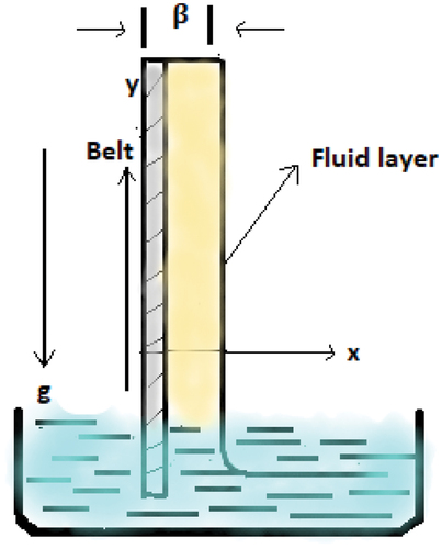
Table 1. Thermophysical properties of base fluid and nanoparticles.

Base fluid/Nanoparticles	$\rho (kg/m^3)$	$C_p(J/kgK)$
Copper	18933	385
Water	997	4179

The governing equations of incompressible Johnson-Segalman nanofluid are [53]

(16) $div\mathcal{V}=0,$(16)

(17) ${\rho }_{nf}\frac{D\mathcal{V}}{Dt}=div(\sigma )+{\rho }_{nf}\mathfrak{f},$(17)

where $\mathcal{V}$ denotes the fluid velocity vector, $\mathfrak{f}$ the body force per unit mass, ${\rho }_{nf}$ is the constant density, $\frac{D}{Dt}$ the material time derivative, and $\sigma$ is the Cauchy stress tensor which is related to fluid motion through following relation

(18) $\sigma =-p\mathcal{I}+\mathcal{T},$(18)

(19) $\mathcal{T}=\mathbb{S}+2\mu \mathcal{D},$(19)

where $\mathcal{T}$ is the total stress tensor, $\mathbb{S}$ is the extra stress tensor, $\mathcal{D}$ is the rate-of-deformation that represents the strain rate in the fluid and parameter $\mu$ is related to the fluid viscosity.

(20) $\mathbb{S}+m\left[\frac{D\mathbb{S}}{Dt}+\mathbb{S}(\mathcal{W}-\lambda \mathcal{D})+{(\mathcal{W}-\lambda \mathcal{D})}^T\mathbb{S}\right]=2\eta \mathcal{D},$(20)

where parameter $m$ represents the viscoelasticity strength of the fluid, $\lambda$ is related to the fluid viscoelastic behaviour, $\mathcal{W}$ is the velocity gradient tensor that represents the local rate of change in velocity and $\eta$ is related to the viscoelasticity relaxation time of the fluid.

The boundary conditions are

(21) $\vartheta =U_0,atX=0$(21)

$T_{XY}=0,atX=\beta .$

Velocity $(\mathbf{V})$ is of the form

(22) $\mathcal{V}=(0,\vartheta (X),0)$(22)

(23) $\mathcal{T}=\mathcal{T}(X)$(23)

where, $\vartheta$ is velocity and shear stress tensor is $\mathcal{T}=\mathcal{T}(X)$. By substituting (22) into (16) and (17), (16) is satisfied and (17) reduces to:

(24) $0=\frac{d{\mathcal{T}}_{XX}}{dX}+{\rho }_{nf}{\mathfrak{f}}_1,$(24)

(25) $0=\frac{d{\mathcal{T}}_{XY}}{dX}+{\rho }_{nf}{\mathfrak{f}}_2,$(25)

where ${\mathfrak{f}}_1$ and ${\mathfrak{f}}_2$ are the body force components. Since, y-coordinate is upward while gravitational force$(\mathfrak{g})$ is downward; hence, above equation becomes

(26) $\frac{0=d{\mathcal{T}}_{XX}}{dX,}$(26)

(27) $0=\frac{d{\mathcal{T}}_{XY}}{dX}-{\rho }_{nf}\mathfrak{g}.$(27)

Using (22) and (23) in (20), components of $\mathbb{S}$ are

(28) ${\mathbb{S}}_{XX}=\frac{-\eta m(1-\lambda ){\left(\frac{d\vartheta }{dX}\right)}^2}{1+m^2(1-{\lambda }^2){\left(\frac{d\vartheta }{dX}\right)}^2},$(28)

(29) ${\mathbb{S}}_{XY}=\frac{\eta \left(\frac{d\vartheta }{dX}\right)}{1+m^2(1-{\lambda }^2){\left(\frac{d\vartheta }{dX}\right)}^2}={\mathbb{S}}_{YX},$(29)

(30) ${\mathbb{S}}_{YY}=\frac{\eta m(1+\lambda ){\left(\frac{d\vartheta }{dX}\right)}^2}{1+m^2(1-{\lambda }^2){\left(\frac{d\vartheta }{dX}\right)}^2}$(30)

Using (28),(29) and (30), tensor $\mathcal{T}$ (19) becomes

(31) ${\mathcal{T}}_{XX}=\frac{-\eta m(1-\lambda ){\left(\frac{d\vartheta }{dX}\right)}^2}{1+m^2(1-{\lambda }^2){\left(\frac{d\vartheta }{dX}\right)}^2},$(31)

(32) ${\mathcal{T}}_{XY}={\mu }_{nf}\left(\frac{d\vartheta }{dX}\right)+\frac{\eta \left(\frac{d\vartheta }{dX}\right)}{1+m^2(1-{\lambda }^2){\left(\frac{d\vartheta }{dX}\right)}^2}={\mathcal{T}}_{YX},$(32)

(33) ${\mathcal{T}}_{YY}=\frac{\eta m(1+\lambda ){\left(\frac{d\vartheta }{dX}\right)}^2}{1+m^2(1-{\lambda }^2){\left(\frac{d\vartheta }{dX}\right)}^2}$(33)

Using (32) into (27) gives

(34) $\frac{d}{dX}\left[{\mu }_{nf}\left(\frac{d\vartheta }{dX}\right)+\frac{\eta \left(\frac{d\vartheta }{dX}\right)}{1+m^2(1-{\lambda }^2){\left(\frac{d\vartheta }{dX}\right)}^2}\right]={\rho }_{nf}\mathfrak{g},$(34)

Boundary conditions become

$\vartheta { }^{\mathrm{\prime }}(X)=0,atX=\beta ,$

(35) $\vartheta (X)=U_0,atX=0,$(35)

Introduce non-dimensional parameters in the form

(36) $X^{\ast }=\frac{X}{\beta },{\vartheta }^{\ast }=\frac{\vartheta }{U_0}and\varphi =\frac{{\mu }_f^{\ast }}{{\mu }_f^{\ast }+\eta },where,F_2{\mu }_f={\mu }_f^{\ast },F_2=\frac{{\mu }_{nf}}{{\mu }_f}$(36)

where $\varphi$ denotes the viscosity ratio. Using Eq (36)(36) $X^{\ast }=\frac{X}{\beta },{\vartheta }^{\ast }=\frac{\vartheta }{U_0}and\varphi =\frac{{\mu }_f^{\ast }}{{\mu }_f^{\ast }+\eta },where,F_2{\mu }_f={\mu }_f^{\ast },F_2=\frac{{\mu }_{nf}}{{\mu }_f}$(36) into (34) gives,

(37) $\frac{d}{dX}\left[\varphi \left(\frac{d\vartheta }{dX}\right)+\frac{(1-\varphi )\left(\frac{d\vartheta }{dX}\right)}{1+{\mathbb{W}}_e^2(1-{\lambda }^2){\left(\frac{d\vartheta }{dX}\right)}^2}\right]={\mathbb{S}}_t,$(37)

(38) $\begin{array}{rl}& \vartheta { }^{\mathrm{\prime }}(x)=0,atX=1,\\ & \vartheta (X)=1,atX=0,\end{array}$(38)

Here, ${\mathbb{W}}_e=\frac{m{U}_0}{\beta }$ is a Weissenberg number, ${\tilde{\mathbb{S}}}_t=\frac{{\rho }_f\mathfrak{g}{\beta }^2}{{\mu }_{eff}{U}_0}$ represent Stoke’s numbers, where, ${\mathbb{S}}_t$=$F_1{\tilde{\mathbb{S}}}_t$, $F_1=\frac{{\rho }_{nf}}{{\rho }_f}$ and ${\mu }_{eff}={\mu }_f+\eta$, respectively. Also, $F_1$= $(1-\eta )+\eta \left(\frac{{\rho }_s}{{\rho }_f}\right)$, $F_2$ =$\frac{1}{{(1-\eta )}^{2.5}}$ where $\eta$ presents the volume fraction. Simplifying (37) gives

(39) $\frac{d^2\vartheta }{d{X}^2}+{\left(1-{\lambda }^2\right)}^2{\mathbb{W}}_e^4{\left(\frac{d\vartheta }{dX}\right)}^4\left(\varphi \frac{d^2\vartheta }{d{X}^2}-{\mathbb{S}}_t\right)\text{break}-\left(1-{\lambda }^2\right){\mathbb{W}}_e^2{\left(\frac{d\vartheta }{dX}\right)}^2\left(2{\mathbb{S}}_t+\varphi \frac{d^2\vartheta }{d{X}^2}+\frac{d^2\vartheta }{d{X}^2}\right)-{\mathbb{S}}_t=0$(39)

(40) $\begin{array}{rl}& \frac{d\vartheta }{dX}=0,atX=1\\ & \vartheta =1,atX=0.\end{array}$(40)

To fuzzify this model, we introduce TFNs in the form of $(h_1,h_2,h_3)$ and $(w_1,w_2,w_3)$ for fuzzy parameter ($r-cut$). The discretization used at the boundary has certain flow behaviours due to the fuzziness in boundaries. The fuzzy boundary conditions (BCs) can be further decomposed into interval form using $r-cut$ approach. Thus, the equation(39)(39) $\frac{d^2\vartheta }{d{X}^2}+{\left(1-{\lambda }^2\right)}^2{\mathbb{W}}_e^4{\left(\frac{d\vartheta }{dX}\right)}^4\left(\varphi \frac{d^2\vartheta }{d{X}^2}-{\mathbb{S}}_t\right)\text{break}-\left(1-{\lambda }^2\right){\mathbb{W}}_e^2{\left(\frac{d\vartheta }{dX}\right)}^2\left(2{\mathbb{S}}_t+\varphi \frac{d^2\vartheta }{d{X}^2}+\frac{d^2\vartheta }{d{X}^2}\right)-{\mathbb{S}}_t=0$(39) with uncertain conditions can be written as follows:

(41) $\frac{d^2\tilde{\vartheta }}{d{X}^2}+{\left(1-{\lambda }^2\right)}^2{\mathbb{W}}_e^4{\left(\frac{d\tilde{\vartheta }}{dX}\right)}^4\left(\varphi \frac{d^2\tilde{\vartheta }}{d{X}^2}-{\mathbb{S}}_t\right)\text{break}-\left(1-{\lambda }^2\right){\mathbb{W}}_e^2{\left(\frac{d\tilde{\vartheta }}{dX}\right)}^2\left(2{\mathbb{S}}_t+\varphi \frac{d^2\tilde{\vartheta }}{d{X}^2}+\frac{d^2\tilde{\vartheta }}{d{X}^2}\right)-{\mathbb{S}}_t=0.$(41)

As $0\le r\le 1$, coupled fuzzy differential equations are modelled as

(42) $\begin{array}{rl}& \left[\frac{d^2{u}_1(X;r)}{d{X}^2},\frac{d^2{u}_2(X;r)}{d{X}^2}\right]+(1-{\lambda }^2{)}^2{\mathbb{W}}_e^4{\left(\frac{d{u}_1(X;r)}{dX},\frac{d{u}_2(X;r)}{dX}\right)}^4\left(\varphi \left[\frac{d^2{u}_1(X;r)}{d{X}^2},\frac{d^2{u}_2(z;r)}{d{X}^2}\right]-{\mathbb{S}}_t\right)-\\ & {\mathbb{W}}_e^2{\left(\frac{d{u}_1(X;r)}{dX},\frac{d{u}_2(X;r)}{dX}\right)}^2\left(2{\mathbb{S}}_t+\varphi \left[\frac{d^2{u}_1(X;r)}{d{X}^2},\frac{d^2{u}_2(X;r)}{d{X}^2}\right]+\left[\frac{d^2{u}_1(X;r)}{d{X}^2},\frac{d^2{u}_2(X;r)}{d{X}^2}\right]\right)\end{array}$(42)

$(1-{\lambda }^2)-{\mathbb{S}}_t=0.$

with fuzzy condition

$\tilde{\vartheta }(X;r)=[u_1(X;r),u_2(X;r)]=[h_1+(h_2-h_1)r,h_3-(h_3-h_2)r],atX=0,$

$\frac{d\tilde{\vartheta }(X;r)}{dX}=\left[\frac{d{u}_1(X;r)}{dX},\frac{d{u}_2(X;r)}{dX}\right]=[w_1+(w_2-w_1)r,w_3-(w_3-w_2)r],atX=1,$

where $u_1(X;r)$ and $u_2(X;r)$ are the lower and upper velocity profiles.

By simplifying above equations, we get the coupled system of fuzzy fluid model as

(43) $\begin{array}{rl}& \frac{d^2{u}_1(X;r)}{d{X}^2}+(1-{\lambda }^2{)}^2{\mathbb{W}}_e^4{\left(\frac{d{u}_1(X;r)}{dX}\right)}^4\left(\varphi \frac{d^2{u}_1(X;r)}{d{X}^2}-{\mathbb{S}}_t\right)-{\mathbb{W}}_e^2\\ & (1-{\lambda }^2){\left(\frac{d{u}_1(X;r)}{dX}\right)}^2\left(2{\mathbb{S}}_t+\varphi \frac{d^2{u}_1(X;r)}{d{X}^2}+\frac{d^2{u}_1(X;r)}{d{X}^2}\right)-{\mathbb{S}}_t=0,\end{array}$(43)

$u_1(X;r)=r-1,atX=0$

$\frac{d{u}_1(X;r)}{dX}=r-1,atX=1.$

(44) $\begin{array}{rl}& \frac{d^2{u}_2(X;r)}{d{X}^2}+(1-{\lambda }^2{)}^2{\mathbb{W}}_e^4{\left(\frac{d{u}_2(X;r)}{dX}\right)}^4\left(\varphi \frac{d^2{u}_2(X;r)}{d{X}^2}-{\mathbb{S}}_t\right)-{\mathbb{W}}_e^2\\ & (1-{\lambda }^2){\left(\frac{d{u}_2(X;r)}{dX}\right)}^2\left(2{\mathbb{S}}_t+\varphi \frac{d^2{u}_2(X;r)}{d{X}^2}+\frac{d^2{u}_2(X;r)}{d{X}^2}\right)-{\mathbb{S}}_t=0,\end{array}$(44)

$u_2(X;r)=1-r,atX=0$

$\frac{d{u}_2(X;r)}{dX}=1-r,atX=1.$

Fuzzified He-Laplace Solution in Lifting case

We apply Laplace transform and construct homotopies on coupled fuzzy model ((42)) as

(45) $\begin{array}{rl}& \mathcal{L}\left((1-p)\left[\frac{d^2{u}_1(X;r)}{d{X}^2},\frac{d^2{u}_2(X;r)}{d{X}^2}\right]+p\left(\left[\frac{d^2{u}_1(X;r)}{d{X}^2},\frac{d^2{u}_2(X;r)}{d{X}^2}\right]\right.+{(1-{\lambda }^2)}^2{\mathbb{W}}_e^4\right.\\ & \left[{\left(\frac{d{u}_1(X;r)}{dX}\right)}^4,{\left(\frac{d{u}_2(X;r)}{dX}\right)}^4\right]\left(\varphi \left[\frac{d^2{u}_1(X;r)}{d{X}^2},\frac{d^2{u}_2(X;r)}{d{X}^2}\right]-{\mathbb{S}}_t\right)-{\mathbb{W}}_e^2(1-{\lambda }^2)\\ & \left[{\left(\frac{d{u}_1(X;r)}{dX}\right)}^2,{\left(\frac{d{u}_2(X;r)}{dX}\right)}^2\right]\left(2{\mathbb{S}}_t+\varphi \left[\frac{d^2{u}_1(X;r)}{d{X}^2},\frac{d^2{u}_2(X;r)}{d{X}^2}\right]+\right.\\ & \left.\left.\left.\left[\frac{d^2{u}_1(X;r)}{d{X}^2},\frac{d^2{u}_2(X;r)}{d{X}^2}\right]\right)-{\mathbb{S}}_t\right)\right).\end{array}$(45)

Now, we expand $u_1$ and $u_2$ in Taylor series form as

(46) $u_{1,i}=\sum _{i=0}^{\mathrm{\infty }}{p}^i{u}_{1,i},$(46)

(47) $u_{2,i}=\sum _{i=0}^{\mathrm{\infty }}{p}^i{u}_{2,i},$(47)

where, $u_{1,i}$, $u_{2,i}$ corresponds to the ith-order lower and upper deformation velocities. Substituting (46) and (47) in (45) and comparing coefficients of like powers of p gives the following deformation equations

$0th$-order fuzzy problem and solution

(48) $u{{ }^{\mathrm{\prime }\mathrm{\prime }}}_{1,0}(X)=0,u_{1,0}(0)=r-1,u{{ }^{\mathrm{\prime }}}_{1,0}(1)=r-1,$(48)

(49) $u_{1,0}(X)=rX+r-X-1.$(49)

(50) $u{{ }^{\mathrm{\prime }\mathrm{\prime }}}_{2,0}(X)=0,u_{2,0}(0)=1-r,u{{ }^{\mathrm{\prime }}}_{2,0}(1)=1-r,$(50)

(51) $u_{2,0}(X)=1+X-r-rX.$(51)

$1st$-order fuzzy problem and solution:

(52) $\begin{array}{rl}& {\lambda }^4{\mathbb{W}}_e^4\varphi {u{ }^{\mathrm{\prime }}}_{1,0}(X{)}^4{u{ }^{\mathrm{\prime }\mathrm{\prime }}}_{1,0}(X)-{\lambda }^4{\mathbb{S}}_t{\mathbb{W}}_e^4{u{ }^{\mathrm{\prime }}}_{1,0}(X{)}^4+2{\lambda }^2{\mathbb{S}}_t{W}^4{u{ }^{\mathrm{\prime }}}_{1,0}(X{)}^4\\ & +2{\lambda }^2{\mathbb{S}}_t{\mathbb{W}}_e^2{u{ }^{\mathrm{\prime }}}_{1,0}(X{)}^2-2{\lambda }^2{\mathbb{W}}_e^4\varphi {u{ }^{\mathrm{\prime }}}_{1,0}(X{)}^4{u{ }^{\mathrm{\prime }\mathrm{\prime }}}_{1,0}(X)+{\lambda }^2{\mathbb{W}}_e^2\varphi {u{ }^{\mathrm{\prime }}}_{1,0}(X{)}^2{u{ }^{\mathrm{\prime }\mathrm{\prime }}}_{1,0}(X)\\ & +{\lambda }^2{\mathbb{W}}_e^2{u{ }^{\mathrm{\prime }}}_{1,0}(X{)}^2{u{ }^{\mathrm{\prime }\mathrm{\prime }}}_{1,0}(X)-{\mathbb{S}}_t{\mathbb{W}}_e^4{u{ }^{\mathrm{\prime }}}_{1,0}(X{)}^4-2{\mathbb{S}}_t{\mathbb{W}}_e^2{u{ }^{\mathrm{\prime }}}_{2,0}(X{)}^2\\ & -{\mathbb{S}}_t+{\mathbb{W}}_e^4\varphi {u{ }^{\mathrm{\prime }}}_{2,0}(X{)}^4{u{ }^{\mathrm{\prime }\mathrm{\prime }}}_{1,0}(X)-{\mathbb{W}}_e^2\varphi {u{ }^{\mathrm{\prime }}}_{1,0}(X{)}^2{u{ }^{\mathrm{\prime }\mathrm{\prime }}}_{1,0}(X)-{\mathbb{W}}_e^2{u{ }^{\mathrm{\prime }}}_{1,0}(X{)}^2{u{ }^{\mathrm{\prime }\mathrm{\prime }}}_{1,0}(X)\\ & +{u{ }^{\mathrm{\prime }\mathrm{\prime }}}_{1,1}(X)=0,u_{1,1}(0)=0,{u{ }^{\mathrm{\prime }}}_{1,1}(1)=0,\end{array}$(52)

(53) $u_{1,1}(X)=\frac{1}{2}{\mathbb{S}}_t({\mathbb{W}}_e^2({\lambda }^2-1)(r-1{)}^2-1{)}^2(X-2)X.$(53)

(54) $\begin{array}{rl}& {\lambda }^4{\mathbb{W}}_e^4\varphi {u{ }^{\mathrm{\prime }}}_{2,0}(X{)}^4{u{ }^{\mathrm{\prime }\mathrm{\prime }}}_{2,0}(X)-{\lambda }^4{\mathbb{S}}_t{\mathbb{W}}_e^4{u{ }^{\mathrm{\prime }}}_{2,0}(X{)}^4+2{\lambda }^2{\mathbb{S}}_t{W}^4{u{ }^{\mathrm{\prime }}}_{2,0}(X{)}^4+2{\lambda }^2{\mathbb{S}}_t{\mathbb{W}}_e^2{u{ }^{\mathrm{\prime }}}_{2,0}(X{)}^2-\\ & 2{\lambda }^2{\mathbb{W}}_e^4\varphi {u{ }^{\mathrm{\prime }}}_{2,0}(X{)}^4{u{ }^{\mathrm{\prime }\mathrm{\prime }}}_{2,0}(X)+{\lambda }^2{\mathbb{W}}_e^2\varphi {u{ }^{\mathrm{\prime }}}_{2,0}(X{)}^2{u{ }^{\mathrm{\prime }\mathrm{\prime }}}_{2,0}(X)+{\lambda }^2{\mathbb{W}}_e^2{u{ }^{\mathrm{\prime }}}_{2,0}(X{)}^2{u{ }^{\mathrm{\prime }\mathrm{\prime }}}_{2,0}(X)\\ & -{\mathbb{S}}_t{\mathbb{W}}_e^4{u{ }^{\mathrm{\prime }}}_{2,0}(X{)}^4-2{\mathbb{S}}_t{\mathbb{W}}_e^2{u{ }^{\mathrm{\prime }}}_{2,0}(X{)}^2-{\mathbb{S}}_t+{\mathbb{W}}_e^4\varphi {u{ }^{\mathrm{\prime }}}_{2,0}(X{)}^4{u{ }^{\mathrm{\prime }\mathrm{\prime }}}_{2,0}(X)\\ & -{\mathbb{W}}_e^2\varphi {u{ }^{\mathrm{\prime }}}_{2,0}(X{)}^2{u{ }^{\mathrm{\prime }\mathrm{\prime }}}_{2,0}(X)-{\mathbb{W}}_e^2{u{ }^{\mathrm{\prime }}}_{2,0}(X{)}^2{u{ }^{\mathrm{\prime }\mathrm{\prime }}}_{2,0}(X)+\\ & {u{ }^{\mathrm{\prime }\mathrm{\prime }}}_{2,1}(X)=0,u_{2,1}(0)=0,{u{ }^{\mathrm{\prime }}}_{2,1}(1)=0,\end{array}$(54)

(55) $u_{2,1}(X)=\frac{1}{2}{\mathbb{S}}_t({\mathbb{W}}_e^2({\lambda }^2-1)(r-1{)}^2-1{)}^2(X-2)X.$(55)

Second order deformation equation is

(56) $\tilde{\vartheta }=[u_1,u_2]=[u_{1,0},u_{2,0}]+[u_{1,1},u_{2,1}]+[u_{1,2},u_{2,2}]+\dots$(56)

Combining (49)(53) gives series solution at lower bound as

(57) $u_1(X)=rX+r-X-1+1/2{\mathbb{S}}_t({\mathbb{W}}_e^2({\lambda }^2-1)(r-1{)}^2-1{)}^2(X-2)X-1/6({\lambda }^2-1)(r-1){\mathbb{S}}_t{\mathbb{W}}_e^{2}X(({\lambda }^2-1)\text{break}(r-1{)}^2{\mathbb{W}}_e^2-1{)}^2(3({\lambda }^2-1)r^3{\mathbb{W}}_e^2(X-2)\varphi -({\lambda }^2-1)r^2{\mathbb{W}}_e^2(4{\mathbb{S}}_t((X-3)X+3)+9(X-2)\varphi )\text{break}+r(8({\lambda }^2-1){\mathbb{S}}_t{\mathbb{W}}_e^2((X-3)X+3)+3(X-2)(3({\lambda }^2-1){\mathbb{W}}_e^2\varphi +\varphi +1))\text{break}-4{\mathbb{S}}_t((X-3)X+3)(({\lambda }^2-1){\mathbb{W}}_e^2-1)-3(X-2)(({\lambda }^2-1){\mathbb{W}}_e^2\varphi +\varphi +1)).$(57)

Similarly, combining (51) and (55) provides series solution at upper bound as

(58) $\begin{array}{rl}& u_2(X)=1+X-r-rX+1/2{\mathbb{S}}_t({\mathbb{W}}_e^2({\lambda }^2-1)(r-1{)}^2-1{)}^2(X-2)X-\frac{1}{6}({\lambda }^2-1)(r-1){\mathbb{S}}_t{\mathbb{W}}_e^{2}X(({\lambda }^2-1)\text{break}(r-1{)}^2{\mathbb{W}}_e^2-1{)}^2(3({\lambda }^2-\\ & 1)r^3{\mathbb{W}}_e^2(x-2)\varphi +({\lambda }^2-1)r^2{\mathbb{W}}_e^2(4{\mathbb{S}}_t((x-3)x+3)-9(x-\\ & 2)\varphi )+r(3(X-2)(3({\lambda }^2-1){\mathbb{W}}_e^2\varphi +\varphi +1)-8({\lambda }^2-1){\mathbb{S}}_t\\ & {\mathbb{W}}_e^2((X-3)X+3))+4{\mathbb{S}}_t((X-3)X+3)(({\lambda }^2-1){\mathbb{W}}_e^2-1)-\\ & 3(X-2)(({\lambda }^2-1){\mathbb{W}}_e^2\varphi +\varphi +1)).\end{array}$(58)

Fuzzified Flow Rate in Lifting Case

The flow rate at lower and upper bounds are

(59) $\begin{array}{rl}& {\mathcal{Q}}_L=\frac{1}{6}(2r^8\mathrm{S}\mathrm{t}{\tau }^4{\mathbb{W}}_e^8\varphi +r^7{\mathbb{S}}_t{\tau }^4{\mathbb{W}}_e^8(3{\mathbb{S}}_t-16\varphi )-r^6{\mathbb{S}}_t{\tau }^3{\mathbb{W}}_e^6(7\tau {\mathbb{W}}_e^2(3{\mathbb{S}}_t-8\varphi )+2(\varphi -1))+\\ & r^5{\mathbb{S}}_t{\tau }^3{\mathbb{W}}_e^6(9{\mathbb{S}}_t(7\tau {\mathbb{W}}_e^2-1)-4(\varphi (28\tau {\mathbb{W}}_e^2-3)+3))-r^4{\mathbb{S}}_t{\tau }^2{\mathbb{W}}_e^4(35{\tau }^2{\mathbb{W}}_e^4(3{\mathbb{S}}_t-4\varphi )-\\ & 15\tau {\mathbb{W}}_e^2(3{\mathbb{S}}_t-2\varphi +2)+2(\varphi +3))+r^3{\mathbb{S}}_t{\tau }^2{\mathbb{W}}_e^4(3{\mathbb{S}}_t(5\tau {\mathbb{W}}_e^2(7\tau {\mathbb{W}}_e^2-6)+3)+8(-\tau {\mathbb{W}}_e^2\\ & (\varphi (14\tau {\mathbb{W}}_e^2-5)+5)+\varphi +3))-r^2{\mathbb{S}}_t\tau {\mathbb{W}}_e^2(7{\tau }^3{\mathbb{W}}_e^6(9{\mathbb{S}}_t-8\varphi )-30{\tau }^2{\mathbb{W}}_e^4(3{\mathbb{S}}_t-\varphi +1)+\\ & 3\tau {\mathbb{W}}_e^2(9{\mathbb{S}}_t+4\varphi +12)-2(\varphi +3))+r({\mathbb{S}}_t\tau {\mathbb{W}}_e^2(\tau {\mathbb{W}}_e^2-1)(3{\mathbb{S}}_t(\tau {\mathbb{W}}_e^2(7\tau {\mathbb{W}}_e^2-8)+1)+\\ & 4(-\tau {\mathbb{W}}_e^2(4\tau {\mathbb{W}}_e^2\varphi +\varphi +3)+\varphi +3))+9)+{\mathbb{S}}_t(\tau {\mathbb{W}}_e^2-1{)}^2(-{\tau }^2{\mathbb{W}}_e^4(3{\mathbb{S}}_t-2\varphi )+\tau {\mathbb{W}}_e^2\\ & (3{\mathbb{S}}_t+2\varphi +2)-2)-9),\end{array}$(59)

and

(60) $\begin{array}{rl}& {\mathcal{Q}}_U=\frac{1}{6}(-r^5{\mathbb{S}}_t{\tau }^3{\mathbb{W}}_e^6(9{\mathbb{S}}_t(7\tau {\mathbb{W}}_e^2-1)+4\varphi (28\tau {\mathbb{W}}_e^2-3)+12)+2r^8{\mathbb{S}}_t{\tau }^4{\mathbb{W}}_e^8\varphi \\ & -r^7{\mathbb{S}}_t{\tau }^4{\mathbb{W}}_e^8(3{\mathbb{S}}_t+16\varphi )+r^6{\mathbb{S}}_t{\tau }^3{\mathbb{W}}_e^6(7\tau {\mathbb{W}}_e^2(3{\mathbb{S}}_t+8\varphi )-2\varphi +2)\\ & +r^4{\mathbb{S}}_t{\tau }^2{\mathbb{W}}_e^4(35{\tau }^2{\mathbb{W}}_e^4(3{\mathbb{S}}_t+4\varphi )-15\tau {\mathbb{W}}_e^2(3{\mathbb{S}}_t+2\varphi -2)-2(\varphi +3))\\ & -r^3{\mathbb{S}}_t{\tau }^2{\mathbb{W}}_e^4(15{\mathbb{S}}_t\tau {\mathbb{W}}_e^2(7\tau {\mathbb{W}}_e^2-6)+9{\mathbb{S}}_t+8\tau {\mathbb{W}}_e^2(\varphi (14\tau {\mathbb{W}}_e^2-5)+5)-8\varphi -24)\\ & +r^2{\mathbb{S}}_t\tau {\mathbb{W}}_e^2(7{\tau }^3{\mathbb{W}}_e^6(9{\mathbb{S}}_t+8\varphi )-30{\tau }^2{\mathbb{W}}_e^4(3{\mathbb{S}}_t+\varphi -1)+3\tau {\mathbb{W}}_e^2(9{\mathbb{S}}_t-4(\varphi +3))\\ & +2(\varphi +3))+r({\mathbb{S}}_t(-\tau ){\mathbb{W}}_e^2(\tau {\mathbb{W}}_e^2-1)(3(\tau {\mathbb{W}}_e^2-1)({\mathbb{S}}_t(7\tau {\mathbb{W}}_e^2-1)+4)\\ & +4\varphi (4{\tau }^2{\mathbb{W}}_e^4+\tau {\mathbb{W}}_e^2-1))-9)+{\mathbb{S}}_t(\tau {\mathbb{W}}_e^2-1{)}^2({\tau }^2{\mathbb{W}}_e^4(3{\mathbb{S}}_t+2\varphi )\\ & -\tau {\mathbb{W}}_e^2(3{\mathbb{S}}_t-2\varphi -2)-2)+9),\end{array}$(60)

respectively. Where $\tau$ =$({\lambda }^2-1)$.

Formulation of Drainage case in Fuzzy environment

Now, we consider the JSF falling in the opposite direction to gravity. Hence, Eqns (16)(16) $div\mathcal{V}=0,$(16) -(20(20) $\mathbb{S}+m\left[\frac{D\mathbb{S}}{Dt}+\mathbb{S}(\mathcal{W}-\lambda \mathcal{D})+{(\mathcal{W}-\lambda \mathcal{D})}^T\mathbb{S}\right]=2\eta \mathcal{D},$(20) ) become

(61) $0=\frac{d{\mathcal{T}}_{XY}}{dX}+{\rho }_{nf}\mathfrak{g}.$(61)

Using (32) into (27) gives

(62) $\frac{d}{dx}\left[{\mu }_{nf}\left(\frac{d\vartheta }{dX}\right)+\frac{\eta \left(\frac{d\vartheta }{dX}\right)}{1+m^2(1-{\lambda }^2){\left(\frac{d\vartheta }{dX}\right)}^2}\right]=-{\rho }_{nf}\mathfrak{g},$(62)

with

(63) $\begin{array}{rl}& \vartheta { }^{\mathrm{\prime }}(X)=0,atX=\beta ,\\ & \vartheta (X)=0,atX=0,\end{array}$(63)

Eq (61)(61) $0=\frac{d{\mathcal{T}}_{XY}}{dX}+{\rho }_{nf}\mathfrak{g}.$(61) in dimensionless form is

(64) $\frac{d}{dX}\left[\varphi \left(\frac{d\vartheta }{dX}\right)+\frac{(1-\varphi )\left(\frac{d\vartheta }{dX}\right)}{1+{\mathbb{W}}_e^2(1-{\lambda }^2){\left(\frac{d\vartheta }{dX}\right)}^2}\right]=-{\mathbb{S}}_t,$(64)

(65) $\begin{array}{rl}& \vartheta { }^{\mathrm{\prime }}(X)=0,atX=1,\\ & \vartheta (X)=0,atX=0,\end{array}$(65)

Simplifying (64) gives

(66) $\frac{d^2\vartheta }{d{X}^2}+{\left(1-{\lambda }^2\right)}^2{\mathbb{W}}_e^4{\left(\frac{d\vartheta }{dX}\right)}^4\left(\varphi \frac{d^2\vartheta }{d{X}^2}+{\mathbb{S}}_t\right)-\left(1-{\lambda }^2\right){\mathbb{W}}_e^2{\left(\frac{d\vartheta }{dX}\right)}^2\left(-2{\mathbb{S}}_t+\varphi \frac{d^2\vartheta }{d{X}^2}+\frac{d^2\vartheta }{d{X}^2}\right)+{\mathbb{S}}_t=0.$(66)

with

(67) $\begin{array}{rl}& \frac{d\vartheta }{dX}=0,atX=1\\ & \vartheta (X)=0,atX=0.\end{array}$(67)

To fuzzify this model, we use TFNs as $(h_1,h_2,h_3)$ and $(w_1,w_2,w_3)$ for the fuzzy parameter ($r-cut$). The fuzzy boundary conditions (BCs) can be further decomposed into interval form using the $r-cut$ approach. Thus, equation(66)(66) $\frac{d^2\vartheta }{d{X}^2}+{\left(1-{\lambda }^2\right)}^2{\mathbb{W}}_e^4{\left(\frac{d\vartheta }{dX}\right)}^4\left(\varphi \frac{d^2\vartheta }{d{X}^2}+{\mathbb{S}}_t\right)-\left(1-{\lambda }^2\right){\mathbb{W}}_e^2{\left(\frac{d\vartheta }{dX}\right)}^2\left(-2{\mathbb{S}}_t+\varphi \frac{d^2\vartheta }{d{X}^2}+\frac{d^2\vartheta }{d{X}^2}\right)+{\mathbb{S}}_t=0.$(66) with fuzzy conditions can be written as

(68) $\frac{d^2\tilde{\vartheta }}{d{X}^2}+{\left(1-{\lambda }^2\right)}^2{\mathbb{W}}_e^4{\left(\frac{d\tilde{\vartheta }}{dX}\right)}^4\left(\varphi \frac{d^2\tilde{\vartheta }}{d{X}^2}+{\mathbb{S}}_t\right)-\left(1-{\lambda }^2\right){\mathbb{W}}_e^2{\left(\frac{d\tilde{\vartheta }}{dX}\right)}^2\left(-2{\mathbb{S}}_t+\varphi \frac{d^2\tilde{\vartheta }}{d{X}^2}+\frac{d^2\tilde{\vartheta }}{d{X}^2}\right)+{\mathbb{S}}_t=0.$(68)

As $0\le r\le 1$, coupled fuzzy differential equations are

(69) $\begin{array}{rl}& \left[\frac{d^2{u}_1(X;r)}{d{X}^2},\frac{d^2{u}_2(X;r)}{d{X}^2}\right]+(1-{\lambda }^2{)}^2{\mathbb{W}}_e^4{\left(\frac{d{u}_1(X;r)}{dX},\frac{d{u}_2(X;r)}{dX}\right)}^4\left(\varphi \left[\frac{d^2{u}_1(X;r)}{d{X}^2},\frac{d^2{u}_2(z;r)}{d{X}^2}\right]+{\mathbb{S}}_t\right)\\ & -{\mathbb{W}}_e^2{\left(\frac{d{u}_1(X;r)}{dX},\frac{d{u}_2(X;r)}{dX}\right)}^2\left(-2{\mathbb{S}}_t+\varphi \left[\frac{d^2{u}_1(X;r)}{d{X}^2},\frac{d^2{u}_2(X;r)}{d{X}^2}\right]+\left[\frac{d^2{u}_1(X;r)}{d{X}^2},\frac{d^2{u}_2(X;r)}{d{X}^2}\right]\right)\\ & (1-{\lambda }^2)+{\mathbb{S}}_t=0,\end{array}$(69)

with fuzzy conditions

$\tilde{\vartheta }(X;r)=[u_1(X;r),u_2(X;r)]=[h_1+(h_2-h_1)r,h_3-(h_3-h_2)r],atX=0,$

$\frac{d\tilde{\vartheta }(X;r)}{dX}=\left[\frac{d{u}_1(X;r)}{dX},\frac{d{u}_2(X;r)}{dX}\right]=[w_1+(w_2-w_1)r,w_3-(w_3-w_2)r],atX=1.$

By simplifying above equations, we get the coupled system of fuzzy fluid model as

(70) $\begin{array}{rl}& \frac{d^2{u}_1(X;r)}{d{X}^2}+(1-{\lambda }^2{)}^2{\mathbb{W}}_e^4{\left(\frac{d{u}_1(X;r)}{dX}\right)}^4\left(\varphi \frac{d^2{u}_1(X;r)}{d{X}^2}+{\mathbb{S}}_t\right)-{\mathbb{W}}_e^2\\ & (1-{\lambda }^2){\left(\frac{d{u}_1(X;r)}{dX}\right)}^2\left(-2{\mathbb{S}}_t+\varphi \frac{d^2{u}_1(X;r)}{d{X}^2}+\frac{d^2{u}_1(X;r)}{d{X}^2}\right)+{\mathbb{S}}_t=0,\end{array}$(70)

$u_1(X;r)=r-1,atX=0$

$\frac{d{u}_1(X;r)}{dX}=r-1,atX=1.$

(71) $\begin{array}{rl}& \frac{d^2{u}_2(X;r)}{d{X}^2}+(1-{\lambda }^2{)}^2{\mathbb{W}}_e^4{\left(\frac{d{u}_2(X;r)}{dX}\right)}^4\left(\varphi \frac{d^2{u}_2(X;r)}{d{X}^2}+{\mathbb{S}}_t\right)-{\mathbb{W}}_e^2\\ & (1-{\lambda }^2){\left(\frac{d{u}_2(X;r)}{dX}\right)}^2\left(-2{\mathbb{S}}_t+\varphi \frac{d^2{u}_2(X;r)}{d{X}^2}+\frac{d^2{u}_2(X;r)}{d{X}^2}\right)+{\mathbb{S}}_t=0,\end{array}$(71)

$u_2(X;r)=1-r,atX=0$

$\frac{d{u}_2(X;r)}{dX}=1-r,atX=1.$

Fuzzified He-Laplace Solution in Drainage case

We apply Laplace transform and construct the homotopies on coupled fuzzy model ((69)) as

(72) $\begin{array}{rl}& \mathcal{L}\left((1-p)\left[\frac{d^2{u}_1(X;r)}{d{X}^2},\frac{d^2{u}_2(X;r)}{d{X}^2}\right]+pH(x)\mathrm{\hslash }\left(\left[\frac{d^2{u}_1(X;r)}{d{X}^2},\frac{d^2{u}_2(X;r)}{d{X}^2}\right]\text{break}+{(1-{\lambda }^2)}^2{\mathbb{W}}_e^4\right.\right.\left[{\left(\frac{d{u}_1(X;r)}{dX}\right)}^4,{\left(\frac{d{u}_2(X;r)}{dX}\right)}^4\right]\left(\varphi \left[\frac{d^2{u}_1(X;r)}{d{X}^2},\frac{d^2{u}_2(X;r)}{d{X}^2}\right]+{\mathbb{S}}_t\right)-{\mathbb{W}}_e^2(1-{\lambda }^2)\left[{\left(\frac{d{u}_1(X;r)}{dX}\right)}^2,{\left(\frac{d{u}_2(X;r)}{dX}\right)}^2\right]\text{break}\left(-2{\mathbb{S}}_t+\varphi \left[\frac{d^2{u}_1(X;r)}{d{X}^2},\frac{d^2{u}_2(X;r)}{d{X}^2}\right]+\right.\\ & \left.\left.\left.\left[\frac{d^2{u}_1(X;r)}{d{X}^2},\frac{d^2{u}_2(X;r)}{d{X}^2}\right]\right)+{\mathbb{S}}_t\right)\right).\end{array}$(72)

Now, we expand $u_1$ and $u_2$ in Taylor series form as

(73) $u_{1,i}=\sum _{i=0}^{\mathrm{\infty }}{p}^i{u}_{1,i},$(73)

(74) $u_{2,i}=\sum _{i=0}^{\mathrm{\infty }}{p}^i{u}_{2,i},$(74)

where, $u_{1,i}$, $u_{2,i}$ corresponds to the ith-order lower and upper deformation velocity profiles. Substituting (73) and (74) in (45) and comparing coefficients of like powers of $p$ gives the following deformation equations

$0th$-order fuzzy problem and solution

(75) $u{{ }^{\mathrm{\prime }\mathrm{\prime }}}_{1,0}(X)=0,u_{1,0}(0)=r-1,u{{ }^{\mathrm{\prime }}}_{1,0}(1)=r-1.$(75)

(76) $u_{1,0}(X)=rX+r-X-1$(76)

(77) $u{{ }^{\mathrm{\prime }\mathrm{\prime }}}_{2,0}(X)=0,u_{2,0}(0)=1-r,u{{ }^{\mathrm{\prime }}}_{2,0}(1)=1-r.$(77)

(78) $u_{2,0}(X)=1+X-r-rX$(78)

$1st$-order fuzzy problem and solution

(79) $\begin{array}{rl}& {\lambda }^4{\mathbb{W}}_e^4\varphi {u{ }^{\mathrm{\prime }}}_{1,0}(X{)}^4{u{ }^{\mathrm{\prime }\mathrm{\prime }}}_{1,0}(X)+{\lambda }^4{\mathbb{S}}_t{\mathbb{W}}_e^4{u{ }^{\mathrm{\prime }}}_{1,0}(X{)}^4-2{\lambda }^2{\mathbb{S}}_t{\mathbb{W}}_e^4{u{ }^{\mathrm{\prime }}}_{1,0}(X{)}^4-2{\lambda }^2{\mathbb{S}}_t{\mathbb{W}}_e^2{u{ }^{\mathrm{\prime }}}_{1,0}(X{)}^2\\ & -2{\lambda }^2{\mathbb{W}}_e^4\varphi {u{ }^{\mathrm{\prime }}}_{1,0}(X{)}^4{u{ }^{\mathrm{\prime }\mathrm{\prime }}}_{1,0}(X)+{\lambda }^2{\mathbb{W}}_e^2\varphi {u{ }^{\mathrm{\prime }}}_{1,0}(X{)}^2{u{ }^{\mathrm{\prime }\mathrm{\prime }}}_{1,0}(X)+{\lambda }^2{\mathbb{W}}_e^2{u{ }^{\mathrm{\prime }\mathrm{\prime }}}_{1,0}(X{)}^2{u{ }^{\mathrm{\prime }\mathrm{\prime }}}_{1,0}(X)+{\mathbb{S}}_t{\mathbb{W}}_e^4{u{ }^{\mathrm{\prime }}}_{1,0}(X{)}^4\\ & +2{\mathbb{S}}_t{\mathbb{W}}_e^2{u{ }^{\mathrm{\prime }}}_{1,0}(X{)}^2+{\mathbb{S}}_t+{\mathbb{W}}_e^4\varphi {u{ }^{\mathrm{\prime }}}_{1,0}(X{)}^4{u{ }^{\mathrm{\prime }\mathrm{\prime }}}_{1,0}(X)-{\mathbb{W}}_e^2\varphi {u{ }^{\mathrm{\prime }}}_{1,0}(X{)}^2{u{ }^{\mathrm{\prime }\mathrm{\prime }}}_{1,0}(X)-{\mathbb{W}}_e^2{u{ }^{\mathrm{\prime }}}_{1,0}(X{)}^2{u{ }^{\mathrm{\prime }\mathrm{\prime }}}_{1,0}(X)\\ & +{u{ }^{\mathrm{\prime }\mathrm{\prime }}}_{1,1}(X)=0,u_{1,1}(0)=0,{u{ }^{\mathrm{\prime }}}_{1,1}(1)=0.\end{array}$(79)

(80) $u_{1,1}(X)=\frac{1}{2}{\mathbb{S}}_t({\mathbb{W}}_e^2({\lambda }^2-1)(r-1{)}^2-1{)}^2(X-2)X$(80)

(81) $\begin{array}{rl}& {\lambda }^4{\mathbb{W}}_e^4\varphi {u{ }^{\mathrm{\prime }}}_{2,0}(X{)}^4{u{ }^{\mathrm{\prime }\mathrm{\prime }}}_{2,0}(X)+{\lambda }^4{\mathbb{S}}_t{\mathbb{W}}_e^4{u{ }^{\mathrm{\prime }}}_{2,0}(X{)}^4-2{\lambda }^2{\mathbb{S}}_t{\mathbb{W}}_e^4{u{ }^{\mathrm{\prime }}}_{2,0}(X{)}^4-2{\lambda }^2{\mathbb{S}}_t{\mathbb{W}}_e^2{u{ }^{\mathrm{\prime }}}_{2,0}(X{)}^2\\ & -2{\lambda }^2{\mathbb{W}}_e^4\varphi {u{ }^{\mathrm{\prime }}}_{2,0}(X{)}^4{u{ }^{\mathrm{\prime }\mathrm{\prime }}}_{2,0}(X)+{\lambda }^2{\mathbb{W}}_e^2\varphi {u{ }^{\mathrm{\prime }}}_{2,0}(X{)}^2{u{ }^{\mathrm{\prime }\mathrm{\prime }}}_{2,0}(X)+{\lambda }^2{\mathbb{W}}_e^2{u{ }^{\mathrm{\prime }}}_{2,0}(X{)}^2{u{ }^{\mathrm{\prime }\mathrm{\prime }}}_{2,0}(X)+{\mathbb{S}}_t{\mathbb{W}}_e^4{u{ }^{\mathrm{\prime }}}_{2,0}(X{)}^4\\ & +2{\mathbb{S}}_t{\mathbb{W}}_e^2{u{ }^{\mathrm{\prime }}}_{2,0}(X{)}^2+{\mathbb{S}}_t+{\mathbb{W}}_e^4\varphi {u{ }^{\mathrm{\prime }}}_{2,0}(X{)}^4{u{ }^{\mathrm{\prime }\mathrm{\prime }}}_{2,0}(X)-{\mathbb{W}}_e^2\varphi {u{ }^{\mathrm{\prime }}}_{2,0}(X{)}^2{u{ }^{\mathrm{\prime }\mathrm{\prime }}}_{2,0}(X)-{\mathbb{W}}_e^2{u{ }^{\mathrm{\prime }}}_{2,0}(X{)}^2{u{ }^{\mathrm{\prime }\mathrm{\prime }}}_{2,0}(X)\\ & +{u{ }^{\mathrm{\prime }\mathrm{\prime }}}_{2,1}(X)=0,u_{2,1}(0)=0,{u{ }^{\mathrm{\prime }}}_{2,1}(1)=0.\end{array}$(81)

(82) $u_{2,1}(X)=\frac{1}{2}{\mathbb{S}}_t({\mathbb{W}}_e^2({\lambda }^2-1)(r-1{)}^2-1{)}^2(X-2)X$(82)

Second order deformation equation is

(83) $\tilde{\vartheta }=[u_1,u_2]=[u_{1,0},u_{2,0}]+[u_{1,1},u_{2,1}]+[u_{1,2},u_{2,2}]+\dots$(83)

Combining Eq (76)(76) $u_{1,0}(X)=rX+r-X-1$(76) and (80(80) $u_{1,1}(X)=\frac{1}{2}{\mathbb{S}}_t({\mathbb{W}}_e^2({\lambda }^2-1)(r-1{)}^2-1{)}^2(X-2)X$(80) ) leads to series form solution at lower bound as

(84) $\begin{array}{rl}& u_1(X;r)=rX+r-X-1+1/2{\mathbb{S}}_t({\mathbb{W}}_e^2({\lambda }^2-1)(r-1{)}^2-1{)}^2(X-2)X+1/6(-1+{\lambda }^2)\\ & (-1+r){\mathbb{S}}_t{\mathbb{W}}_e^2(-1+(-1+{\lambda }^2)(-1+r{)}^2{\mathbb{W}}_e^2{)}^{2}X(4{\mathbb{S}}_t(-1+({\lambda }^2-1){\mathbb{W}}_e^2)(3+(-3+x)x)\\ & +3(-1+{\lambda }^2)r^3{\mathbb{W}}_e^2(-2+X)\varphi -3(-2+X)(1+\varphi +(-1+{\lambda }^2){\mathbb{W}}_e^2\varphi )+(-1+{\lambda }^2)r^2\\ & {\mathbb{W}}_e^2(4{\mathbb{S}}_t(3+(-3+X)X)-9(-2+X)\varphi )+r(-8(-1+{\lambda }^2){\mathbb{S}}_t{\mathbb{W}}_e^2(3+(-3+X)X)\\ & +3(-2+X)(1+\varphi +3(-1+{\lambda }^2){\mathbb{W}}_e^2\varphi ))).\end{array}$(84)

Similarly, combining Eq (78)(78) $u_{2,0}(X)=1+X-r-rX$(78) and (82(82) $u_{2,1}(X)=\frac{1}{2}{\mathbb{S}}_t({\mathbb{W}}_e^2({\lambda }^2-1)(r-1{)}^2-1{)}^2(X-2)X$(82) ) leads to a solution at upper bound as

(85) $\begin{array}{rl}& u_2(X;r)=1+X-r-rX+1/2{\mathbb{S}}_t({\mathbb{W}}_e^2({\lambda }^2-1)(r-1{)}^2-1{)}^2(X-2)X+1/6(-1+{\lambda }^2)\\ & (-1+r){\mathbb{S}}_t{\mathbb{W}}_e^2(-1+(-1+{\lambda }^2)(-1+r{)}^2{\mathbb{W}}_e^2{)}^{2}X(-4{\mathbb{S}}_t(-1+(-1+{\lambda }^2){\mathbb{W}}_e^2)(3+(-3+X)X)\\ & +3(-1+{\lambda }^2)r^3{\mathbb{W}}_e^2(-2+X)\varphi -3(-2+X)(1+\varphi +(-1+{\lambda }^2){\mathbb{W}}_e^2\varphi )-(-1+{\lambda }^2)r^2\\ & {\mathbb{W}}_e^2(4{\mathbb{S}}_t(3+(-3+X)X)+9(-2+X)\varphi )+r(-8(-1+{\lambda }^2){\mathbb{S}}_t{\mathbb{W}}_e^2(3+(-3+X)X)\\ & +3(-2+X)(1+\varphi +3(-1+{\lambda }^2){\mathbb{W}}_e^2\varphi ))).\end{array}$(85)

Fuzzified Average Velocity and Flow Rate in Draining Case

The flow rate at lower and upper bounds are

(86) $\begin{array}{rl}& {\mathcal{Q}}_L=\frac{1}{6}(-2r^8\mathrm{S}\mathrm{t}{\tau }^4{\mathbb{W}}_e^8\varphi +r^7\mathrm{S}\mathrm{t}{\tau }^4{\mathbb{W}}_e^8(3\mathrm{S}\mathrm{t}+16\varphi )-r^6\mathrm{S}\mathrm{t}{\tau }^3{\mathbb{W}}_e^6(7\tau {\mathbb{W}}_e^2(3\mathrm{S}\mathrm{t}+8\varphi )-2\varphi +2)\\ & +r^5\mathrm{S}\mathrm{t}{\tau }^3{\mathbb{W}}_e^6(9\mathrm{S}\mathrm{t}(7\tau {\mathbb{W}}_e^2-1)+4\varphi (28\tau {\mathbb{W}}_e^2-3)+12)-r^4\mathrm{S}\mathrm{t}{\tau }^2{\mathbb{W}}_e^4(35{\tau }^2{\mathbb{W}}_e^4(3\mathrm{S}\mathrm{t}+4\varphi )\\ & -15\tau {\mathbb{W}}_e^2(3\mathrm{S}\mathrm{t}+2\varphi -2)-2(\varphi +3))+r^3\mathrm{S}\mathrm{t}{\tau }^2{\mathbb{W}}_e^4(15\mathrm{S}\mathrm{t}\tau {\mathbb{W}}_e^2(7\tau {\mathbb{W}}_e^2-6)+9\mathrm{S}\mathrm{t}+8\tau {\mathbb{W}}_e^2\\ & (\varphi (14\tau W^2-5)+5)-8\varphi -24)-r^2\mathrm{S}\mathrm{t}\tau {\mathbb{W}}_e^2(7{\tau }^3{\mathbb{W}}_e^6(9\mathrm{S}\mathrm{t}+8\varphi )-30{\tau }^2{\mathbb{W}}_e^4(3\mathrm{S}\mathrm{t}+\varphi -1)\\ & +3\tau {\mathbb{W}}_e^2(9\mathrm{S}\mathrm{t}-4(\varphi +3))+2(\varphi +3))+r(\mathrm{S}\mathrm{t}\tau {\mathbb{W}}_e^2(\tau {\mathbb{W}}_e^2-1)(3(\tau W^2-1)(\mathrm{S}\mathrm{t}(7\tau {\mathbb{W}}_e^2-1)+4)\\ & +4\varphi (4{\tau }^2{\mathbb{W}}_e^4+\tau {\mathbb{W}}_e^2-1))+9)+\mathrm{S}\mathrm{t}(\tau {\mathbb{W}}_e^2-1{)}^2(-{\tau }^2{\mathbb{W}}_e^4(3\mathrm{S}\mathrm{t}+2\varphi )+\tau {\mathbb{W}}_e^2(3\mathrm{S}\mathrm{t}-2\varphi -2)+2)-9),\end{array}$(86)

and

(87) $\begin{array}{rl}& {\mathcal{Q}}_U=\frac{1}{6}(-2r^8\mathrm{S}\mathrm{t}{\tau }^4{\mathbb{W}}_e^8\varphi -r^7\mathrm{S}\mathrm{t}{\tau }^4{\mathbb{W}}_e^8(3\mathrm{S}\mathrm{t}-16\varphi )+r^6\mathrm{S}\mathrm{t}{\tau }^3{\mathbb{W}}_e^6(7\tau {\mathbb{W}}_e^2(3\mathrm{S}\mathrm{t}-8\varphi )+2\varphi -1)\\ & +r^5\mathrm{S}\mathrm{t}{\tau }^3{\mathbb{W}}_e^6(9\mathrm{S}\mathrm{t}(7\tau {\mathbb{W}}_e^2-1)-4(\varphi (28\tau {\mathbb{W}}_e^2-3)+3))+r^4\mathrm{S}\mathrm{t}{\tau }^2{\mathbb{W}}_e^4(35{\tau }^2{\mathbb{W}}_e^4(3\mathrm{S}\mathrm{t}-4\varphi )\\ & -15\tau {\mathbb{W}}_e^2(3\mathrm{S}\mathrm{t}-2\varphi +2)+2(\varphi +3))-r^3\mathrm{S}\mathrm{t}{\tau }^2{\mathbb{W}}_e^4(15\mathrm{S}\mathrm{t}\tau {\mathbb{W}}_e^2(7\tau {\mathbb{W}}_e^2-6)+9\mathrm{S}\mathrm{t}+8\tau {\mathbb{W}}_e^2\\ & (-(\varphi (14\tau {\mathbb{W}}_e^2-5)+5))+\varphi +3))+r^2\mathrm{S}\mathrm{t}\tau {\mathbb{W}}_e^2(7{\tau }^3{\mathbb{W}}_e^6(9\mathrm{S}\mathrm{t}-8\varphi )-30{\tau }^2{\mathbb{W}}_e^4(3\mathrm{S}\mathrm{t}-\varphi +1)\\ & +3\tau {\mathbb{W}}_e^2(9\mathrm{S}\mathrm{t}+4\varphi +12)-2(\varphi +3))+r(-\mathrm{t}\mathrm{S}\mathrm{t}{\mathbb{W}}_e^2(\tau {\mathbb{W}}_e^2-1)(3\mathrm{S}\mathrm{t}(\tau {\mathbb{W}}_e^2(7\tau {\mathbb{W}}_e^2-8)+1)\\ & +4(-\tau {\mathbb{W}}_e^2(4\tau {\mathbb{W}}_e^2\varphi +\varphi +3)+\varphi +3))-9)+\mathrm{S}\mathrm{t}(\tau {\mathbb{W}}_e^2-1{)}^2({\tau }^2{\mathbb{W}}_e^4(3\mathrm{S}\mathrm{t}-2\varphi )-\tau \\ & {\mathbb{W}}_e^2(3\mathrm{S}\mathrm{t}+2\varphi +2)+2)+9),\end{array}$(87)

respectively. Where, $\tau$ =$({\lambda }^2-1)$.

Results and Discussion

This manuscript presents an analysis of Fuzzified Jhonson Segalman nanofluid in lifting and drainage cases. The effects of various parameters (fluid and fuzzy parameters) on the velocity profile are examined through graphical and tabular analysis. Tables 2–5 illustrate the impact of different fluid and fuzzy parameters on fluid velocity in lifting case. Similarly, Tables 7–10 display the results for draining case. Table 6 respresents fuzzy flow rate in lifting and drainage cases.These tabulated quantities provide information about fuzzy velocity at lower and upper bounds along with residual errors. Considering factors such as viscosity ratio $\varphi$ for an $r-cut$ value of 0.7 (Tables 2 and 7), Stoke’s number ${\mathbb{S}}_t$ for an $r-cut$ value of 0.35 (Tables 3 and 8), slip parameter $\lambda$ (Tables 4 and 9) and Weissenberg number $\mathbb{W}e$ (Tables 5 and 10). The residual errors in these table 2-10 confirms that obtained fuzzy solutions are consistent, and accurate up to an order of ${10}^{-10}$. Table 11 presentes the comparison of HLM and ADM. Furthermore, Table 4 presents the volumetric flow rate at lower and upper bound in both lifting and drainage cases with fixed fluid parameters. To validate the convergence and stability of the proposed scheme, a comparison with an existing literature is provided in Table 9. The results show that the flow rate decreases as $r-cut$ increases in both lifting and drainage cases. Additionally, the equality of lower and upper bound solutions at $r=1$ confirms the validity of obtained results.

Table 2. Fuzzy solutions and residual errors for the influence of $\varphi$ (lifting problem) when $r=0.7$ ${\mathbb{W}}_e$ = 0.01, ${\mathbb{S}}_t$ = 0.001 and $\lambda$ = 0.1.

		$\varphi =0.1$		$\varphi =0.5$		$\varphi =0.8$
$r=0.7$	$X$	Solution	Error	Solution	Error	Solution	Error
(lower bound)	$0.0$	$-0.3$	$-$6.57$\times {10}^{-11}$	$-0.3000000$	$-$8.97$\times {10}^{-11}$	$-0.3000000$	$-$1.07$\times {10}^{-10}$
	$0.2$	$-0.360180$	$-$5.26$\times {10}^{-11}$	$-0.3601800$	$-$7.17$\times {10}^{-11}$	$-0.360180$	$-$8.60$\times {10}^{-11}$
	$0.4$	$-0.4203200$	$-$3.94$\times {10}^{-11}$	$-0.4203200$	$-$5.37$\times {10}^{-11}$	$-0.4203200$	$-$6.45$\times {10}^{-11}$
	$0.6$	$-0.4804200$	−2.63$\times {10}^{-11}$	$-0.4804200$	$-$3.59$\times {10}^{-11}$	$-0.4804200$	$-$4.30$\times {10}^{-11}$
	$0.8$	$-0.5404800$	$-$1.31$\times {10}^{-11}$	$-0.5704950$	$-$1.80$\times {10}^{-13}$	$-0.5404800$	$-$2.17$\times {10}^{-13}$
	$1.0$	$-0.600500$	$-$9.60$\times {10}^{-14}$	$-0.0073508$	$-$1.79$\times {10}^{-13}$	$-0.6005000$	$-$2.57$\times {10}^{-13}$
(upper bound)	$0.0$	$0.3000000$	6.50$\times {10}^{-11}$	$0.3000000$	8.85$\times {10}^{-11}$	$0.3000000$	1.06$\times {10}^{-11}$
	$0.2$	$0.3598199$	5.19$\times {10}^{-11}$	$0.3598199$	7.08$\times {10}^{-11}$	$0.35981999$	8.50$\times {10}^{-11}$
	$0.4$	$0.4196799$	3.90$\times {10}^{-11}$	$0.4196799$	5.31$\times {10}^{-11}$	$0.4196799$	6.37$\times {10}^{-11}$
	$0.6$	$0.479579$	2.62$\times {10}^{-11}$	$0.479579$	3.54$\times {10}^{-11}$	$0.4795799$	4.25$\times {10}^{-11}$
	$0.8$	$0.5395199$	1.29$\times {10}^{-11}$	$0.5395199$	1.76$\times {10}^{-11}$	$0.5395199$	2.11$\times {10}^{-11}$
	$1.0$	$0.5994999$	$-$9.61$\times {10}^{-14}$	$0.5994999$	$-$1.79$\times {10}^{-13}$	$0.5994999$	$-$2.57$\times {10}^{-13}$

Table 3. Fuzzy solutions and residual errors for the influence of ${\mathbb{S}}_t$ (lifting problem) when ${\mathbb{W}}_e$ = 0.001, $\varphi$ = 0.3 and $\lambda =\frac{1}{8}$.

		${\mathbb{S}}_t=0.001$		${\mathbb{S}}_t=0.01$		${\mathbb{S}}_t=0.1$
$r=0.2$	$X$	Solution	Error	Solution	Error	Solution	Error
(lower bound)	$0.0$	$-0.8$	$-$2.05$\times {10}^{-12}$	$-0.8$	$-$2.08$\times {10}^{-10}$	$-0.8$	$-$2.37$\times {10}^{-8}$
	$0.2$	$-0.960180$	$-$1.64$\times {10}^{-12}$	$-0.961800$	$-$1.66$\times {10}^{-10}$	$-0.978000$	$-$1.84$\times {10}^{-8}$
	$0.4$	$-1.120320$	$-$1.23$\times {10}^{-12}$	$-1.123200$	$-$1.24$\times {10}^{-11}$	$-1.152000$	$-$1.34$\times {10}^{-9}$
	$0.6$	$-1.280420$	$-$8.20$\times {10}^{-13}$	$-1.284200$	$-$8.24$\times {10}^{-11}$	$-1.3220000$	$-$8.71$\times {10}^{-9}$
	$0.8$	$-1.440480$	$-$4.10$\times {10}^{-13}$	$-1.444800$	$-$4.11$\times {10}^{-11}$	$-1.488000$	$-$4.23$\times {10}^{-9}$
	$1.0$	$-1.600500$	$-$6.71$\times {10}^{-16}$	$-1.605000$	$-$6.71$\times {10}^{-15}$	$-1.650000$	$-$6.71$\times {10}^{-14}$
(upper bound)	$0.0$	$0.8$	2.04$\times {10}^{-12}$	$0.8$	2.01$\times {10}^{-10}$	$0.8$	1.72$\times {10}^{-8}$
	$0.2$	$0.9598199$	1.63$\times {10}^{-12}$	$0.9581999$	1.61$\times {10}^{-10}$	$0.941999$	1.43$\times {10}^{-8}$
	$0.4$	$1.11967999$	1.22$\times {10}^{-12}$	$1.1167999$	1.21$\times {10}^{-11}$	$1.0879999$	1.11$\times {10}^{-9}$
	$0.6$	$1.2795799$	8.17$\times {10}^{-13}$	$1.2757999$	8.13$\times {10}^{-11}$	$1.2379999$	7.67$\times {10}^{-9}$
	$0.8$	$1.4395199$	4.08$\times {10}^{-13}$	$1.4351999$	4.08$\times {10}^{-11}$	$1.3919999$	3.97$\times {10}^{-9}$
	$1.0$	$1.599499$	$-$6.71$\times {10}^{-16}$	$1.5949999$	$-$6.71$\times {10}^{-15}$	$1.549999$	$-$6.71$\times {10}^{-14}$

Table 4. Fuzzy solutions and residual errors of the membership function under the influence of $\lambda$ (lifting problem) when ${\mathbb{S}}_t$ = 0.001 ${\mathbb{W}}_e$ = 0.002 and $\varphi =0.03$.

		$\lambda =0.3$		$\lambda =0.6$		$\lambda =0.9$
$X=1.0$	$r$	Solution	Error	Solution	Error	Solution	Error
(lower bound)	$0.0$	$-2.0005$	$-$1.38$\times {10}^{-14}$	$-2.0005$	$-$6.81$\times {10}^{-15}$	$-2.0005$	$-$6.01$\times {10}^{-16}$
	$0.2$	$-1.6005$	$-$5.65$\times {10}^{-15}$	$-1.6005$	$-$2.79$\times {10}^{-15}$	$-1.6005$	$-$2.46$\times {10}^{-16}$
	$0.4$	$-1.2005$	$-$1.79$\times {10}^{-15}$	$-1.2005$	$-$8.84$\times {10}^{-15}$	$-1.2005$	$-$7.77$\times {10}^{-17}$
	$0.6$	$-0.8005$	$-$3.53$\times {10}^{-16}$	$-0.8005$	$-$1.75$\times {10}^{-16}$	$-0.8005$	$-$1.56$\times {10}^{-17}$
	$0.8$	$-0.4005$	$-$2.21$\times {10}^{-17}$	$-0.4005$	$-$1.09$\times {10}^{-17}$	$-0.4005$	$-$7.84$\times {10}^{-19}$
	$1.0$	$-0.0005$	$-$4.82$\times {10}^{-25}$	$-0.0005$	2.80$\times {10}^{-25}$	$-0.0005$	$-$2.17$\times {10}^{-25}$
(upper bound)	$0.0$	$1.995$	$-$1.38$\times {10}^{-14}$	$1.995$	$-$6.81$\times {10}^{-15}$	$1.995$	$-$6.01$\times {10}^{-16}$
	$0.2$	$1.5995$	$-$5.65$\times {10}^{-15}$	$1.5995$	$-$2.79$\times {10}^{-15}$	$1.5995$	$-$2.46$\times {10}^{-16}$
	$0.4$	$1.1995$	$-$1.79$\times {10}^{-15}$	$1.1995$	$-$8.84$\times {10}^{-15}$	$1.1995$	$-$7.77$\times {10}^{-17}$
	$0.6$	$0.7995$	$-$3.53$\times {10}^{-16}$	$0.7995$	$-$1.75$\times {10}^{-16}$	$0.7995$	$-$1.56$\times {10}^{-17}$
	$0.8$	$0.3995$	$-$2.21$\times {10}^{-17}$	$0.3995$	$-$1.09$\times {10}^{-17}$	$0.3995$	$-$7.84$\times {10}^{-19}$
	$1.0$	$0.0005$	$-$4.82$\times {10}^{-25}$	$0.0005$	2.80$\times {10}^{-25}$	$0.0005$	$-$2.17$\times {10}^{-25}$

Table 5. Fuzzy solutions and residual errors of the membership function under the influence of ${\mathbb{W}}_e$ (lifting problem) when ${\mathbb{S}}_t$ = 0.001 $\lambda$ = 0.99 and $\varphi =0.1$.

		${\mathbb{W}}_e=0.002$		${\mathbb{W}}_e=0.02$		${\mathbb{W}}_e=0.2$
$X=1.0$	$r$	Solution	Error	Solution	Error	Solution	Error
(lower bound)	$0.0$	$-2.0005$	$-$7.74$\times {10}^{-18}$	$-2.0005$	$-$7.67$\times {10}^{-14}$	$-2.0005$	$-$7.68$\times {10}^{-10}$
	$0.2$	$-1.6005$	$-$3.14$\times {10}^{-18}$	$-1.6005$	$-$3.14$\times {10}^{-14}$	$-1.6005$	$-$3.14$\times {10}^{-10}$
	$0.4$	$-1.2005$	$-$1.18$\times {10}^{-18}$	$-1.2005$	$-$9.94$\times {10}^{-15}$	$-1.2005$	$-$9.94$\times {10}^{-11}$
	$0.6$	$-0.8005$	$-$1.98$\times {10}^{-19}$	$-0.8005$	$-$1.96$\times {10}^{-15}$	$-0.8005$	$-$1.96$\times {10}^{-11}$
	$0.8$	$-0.4005$	1.45$\times {10}^{-19}$	$-0.4005$	$-$1.23$\times {10}^{-16}$	$-0.4005$	$-$1.22$\times {10}^{-12}$
	$1.0$	$-0.0005$	2.17$\times {10}^{-19}$	$-0.0005$	$-$2.17$\times {10}^{-19}$	$-0.0005$	$-$2.25$\times {10}^{-19}$
(upper bound)	$0.0$	$1.995$	$-$7.74$\times {10}^{-18}$	$1.995$	$-$7.67$\times {10}^{-14}$	$1.995$	$-$7.68$\times {10}^{-10}$
	$0.2$	$1.5995$	$-$3.14$\times {10}^{-18}$	$1.5995$	$-$3.14$\times {10}^{-14}$	$1.5995$	$-$3.14$\times {10}^{-10}$
	$0.4$	$1.1995$	$-$1.18$\times {10}^{-18}$	$1.1995$	$-$9.94$\times {10}^{-15}$	$1.1995$	$-$9.94$\times {10}^{-11}$
	$0.6$	$0.7995$	$-$1.98$\times {10}^{-19}$	$0.7995$	$-$1.96$\times {10}^{-15}$	$0.7995$	$-$1.96$\times {10}^{-11}$
	$0.8$	$0.3995$	1.45$\times {10}^{-19}$	$0.3995$	$-$1.23$\times {10}^{-16}$	$0.3995$	$-$1.22$\times {10}^{-12}$
	$1.0$	$0.0005$	2.17$\times {10}^{-19}$	$0.0005$	$-$2.17$\times {10}^{-19}$	$0.0005$	$-$2.25$\times {10}^{-19}$

Table 6. Fuzzy flow rate in lifting and drainage case when $\varphi =0.6$, ${\mathbb{W}}_e$ = 0.5, ${\mathbb{S}}_t$ = 0.3 and $\lambda$ = 0.1.

	Flow Rate in Lifting Case		Flow Rate in Draining Case
$r-cut$	${\mathcal{Q}}_L$	${\mathcal{Q}}_U$	${\mathcal{Q}}_L$	${\mathcal{Q}}_U$
$0.0$	$-1.73316$	$1.31009$	$-1.31009$	$1.73316$
$0.2$	$-1.38003$	$1.04767$	$-1.04767$	$1.38003$
$0.4$	$-1.04359$	$0.773674$	$-0.773674$	$1.04359$
$0.6$	$-0.719828$	$0.490183$	$-0.490183$	$0.719828$
$0.8$	$-0.405894$	$0.198695$	$-0.198695$	$0.405894$
$1.0$	$-0.1$	$-0.1$	$0.1$	$0.1$

Table 7. Fuzzy solutions and residual errors for the influence of $\varphi$ (drainage problem) when ${\mathbb{W}}_e$ = 0.01, ${\mathbb{S}}_t$ = 0.001 and $\lambda$ = 0.2.

		$\varphi =0.1$		$\varphi =0.5$		$\varphi =0.7$
$r=0.7$	$X$	Solution	Error	Solution	Error	Solution	Error
(lower bound)	$0.0$	$-0.3$	$-$6.30$\times {10}^{-11}$	$-0.3$	$-$8.59$\times {10}^{-11}$	$-0.3$	$-$9.73$\times {10}^{-11}$
	$0.2$	$-0.35982$	$-$5.04$\times {10}^{-11}$	$-0.35982$	$-$6.87$\times {10}^{-11}$	$-0.35982$	$-$7.79$\times {10}^{-11}$
	$0.4$	$-0.41968$	$-$3.78$\times {10}^{-10}$	$-0.41968$	$-$5.16$\times {10}^{-11}$	$-0.41968$	$-$5.84$\times {10}^{-11}$
	$0.6$	$-0.47958$	$-$2.52$\times {10}^{-11}$	$-0.47958$	$-$3.43$\times {10}^{-11}$	$-0.47958$	$-$3.89$\times {10}^{-11}$
	$0.8$	$-0.53952$	$-$1.26$\times {10}^{-11}$	$-0.53952$	$-$1.71$\times {10}^{-11}$	$-0.53952$	$-$1.94$\times {10}^{-11}$
	$1.0$	$-0.5995$	$9.03\times {10}^{-14}$	$-0.5995$	1.68$\times {10}^{-13}$	$-0.5995$	2.16$\times {10}^{-13}$
(upper bound)	$0.0$	$0.3$	6.38$\times {10}^{-11}$	$0.3$	8.69$\times {10}^{-11}$	$0.3$	9.85$\times {10}^{-11}$
	$0.2$	$0.36018$	5.10$\times {10}^{-11}$	$0.36018$	6.95$\times {10}^{-11}$	$0.36018$	7.88$\times {10}^{-11}$
	$0.4$	$0.42032$	3.82$\times {10}^{-11}$	$0.42032$	5.21$\times {10}^{-11}$	$0.42032$	5.91$\times {10}^{-11}$
	$0.6$	$0.48042$	2.55$\times {10}^{-11}$	$0.48042$	3.48$\times {10}^{-11}$	$0.48042$	3.94$\times {10}^{-11}$
	$0.8$	$0.54048$	1.28$\times {10}^{-11}$	$0.54048$	1.75$\times {10}^{-11}$	$0.54048$	1.98$\times {10}^{-11}$
	$1.0$	$0.6005$	9.03$\times {10}^{-14}$	$0.6005$	1.68$\times {10}^{-13}$	$0.6005$	2.16$\times {10}^{-13}$

Table 8. Fuzzy solutions and residual errors for the influence of ${\mathbb{S}}_t$ (draining problem) when ${\mathbb{W}}_e$ = 0.002, $\varphi$ = 0.3 and $\lambda =0.84$.

		${\mathbb{S}}_t=0.001$		${\mathbb{S}}_t=0.01$		${\mathbb{S}}_t=0.1$
$r=0.35$	$X$	Solution	Error	Solution	Error	Solution	Error
(lower bound)	$0.0$	$-0.65$	$-$7.85$\times {10}^{-13}$	$-0.65$	$-$7.71$\times {10}^{-11}$	$-0.65$	$-$6.33$\times {10}^{-9}$
	$0.2$	$-0.77982$	$-$6.28$\times {10}^{-13}$	$-0.7782$	$-$6.20$\times {10}^{-11}$	$-0.762$	$-$5.31$\times {10}^{-9}$
	$0.4$	$-0.90968$	$-$4.71$\times {10}^{-13}$	$-0.9068$	$-$4.67$\times {10}^{-11}$	$-0.878$	$-$4.17$\times {10}^{-9}$
	$0.6$	$-1.03958$	$-$3.14$\times {10}^{-13}$	$-1.0358$	$-$3.12$\times {10}^{-11}$	$-0.998$	$-$2.90$\times {10}^{-9}$
	$0.8$	$-1.16952$	$-$1.57$\times {10}^{-13}$	$-1.1652$	$-$1.57$\times {10}^{-11}$	$-1.122$	$-$1.51$\times {10}^{-9}$
	$1.0$	$-1.2995$	6.56$\times {10}^{-17}$	$-1.295$	6.54$\times {10}^{-16}$	$-1.25$	6.55$\times {10}^{-15}$
(upper bound)	$0.0$	$0.65$	7.88$\times {10}^{-13}$	$0.65$	8.02$\times {10}^{-11}$	$0.65$	9.41$\times {10}^{-9}$
	$0.2$	$0.78018$	6.31$\times {10}^{-13}$	$0.7818$	6.39$\times {10}^{-11}$	$0.798$	7.28$\times {10}^{-9}$
	$0.4$	$0.91032$	4.73$\times {10}^{-13}$	$0.9132$	4.78$\times {10}^{-11}$	$0.942$	5.27$\times {10}^{-9}$
	$0.6$	$1.04042$	3.15$\times {10}^{-13}$	$1.0442$	3.17$\times {10}^{-11}$	$1.082$	3.39$\times {10}^{-9}$
	$0.8$	$1.17048$	1.57$\times {10}^{-13}$	$1.1748$	1.58$\times {10}^{-11}$	$1.218$	1.63$\times {10}^{-9}$
	$1.0$	$1.3005$	6.56$\times {10}^{-17}$	$1.305$	6.54$\times {10}^{-16}$	$1.35$	6.54$\times {10}^{-15}$

Table 9. Fuzzy solutions and residual errors of the membership function under the influence of $\lambda$ (draining problem) when ${\mathbb{S}}_t$ = 0.001 ${\mathbb{W}}_e$ = 0.002 and $\varphi =0.03$.

		$\lambda =0.3$		$\lambda =0.6$		$\lambda =0.9$
$X=1.0$	$r$	Solution	Error	Solution	Error	Solution	Error
(lower bound)	$0.0$	– 1.995	1.41$\times {10}^{-14}$	– 1.995	6.95$\times {10}^{-15}$	– 1.995	6.13$\times {10}^{-16}$
	$0.2$	– 1.5995	3.76$\times {10}^{-15}$	– 1.5995	2.85$\times {10}^{-15}$	– 1.5995	2.51$\times {10}^{-16}$
	$0.4$	– 1.1995	1.82$\times {10}^{-15}$	– 1.1995	9.01$\times {10}^{-16}$	– 1.1995	7.93$\times {10}^{-17}$
	$0.6$	– 0.7995	3.59$\times {10}^{-16}$	– 0.7995	1.78$\times {10}^{-16}$	– 0.7995	1.59$\times {10}^{-17}$
	$0.8$	– 0.3995	2.26$\times {10}^{-17}$	– 0.3995	1.11$\times {10}^{-17}$	– 0.3995	8.03$\times {10}^{-19}$
	$1.0$	– 0.0005	4.79$\times {10}^{-25}$	– 0.0005	– 2.61$\times {10}^{-25}$	– 0.0005	2.17$\times {10}^{-19}$
(upper bound)	$0.0$	2.0005	1.41$\times {10}^{-14}$	2.0005	6.95$\times {10}^{-15}$	2.0005	6.13$\times {10}^{-16}$
	$0.2$	1.6005	3.76$\times {10}^{-15}$	1.6005	2.85$\times {10}^{-15}$	1.6005	2.51$\times {10}^{-16}$
	$0.4$	1.2005	1.82$\times {10}^{-15}$	1.2005	9.01$\times {10}^{-16}$	1.2005	7.93$\times {10}^{-17}$
	$0.6$	0.8005	3.59$\times {10}^{-16}$	0.8005	1.78$\times {10}^{-16}$	0.8005	1.59$\times {10}^{-17}$
	$0.8$	0.4005	2.26$\times {10}^{-17}$	0.4005	1.11$\times {10}^{-17}$	0.4005	8.03$\times {10}^{-19}$
	$1.0$	0.0005	4.79$\times {10}^{-25}$	0.0005	– 2.61$\times {10}^{-25}$	0.0005	2.17$\times {10}^{-19}$

Table 10. Fuzzy solutions and residual errors of the membership function under the influence of ${\mathbb{W}}_e$ (draining problem) when ${\mathbb{S}}_t$ = 0.001 $\lambda$ = 0.99 and $\varphi =0.11$.

		${\mathbb{W}}_e=0.002$		${\mathbb{W}}_e=0.02$		${\mathbb{W}}_e=0.2$
$X=1.0$	$r$	Solution	Error	Solution	Error	Solution	Error
(lower bound)	$0.0$	– 1.995	7.88$\times {10}^{-18}$	– 1.995	7.80$\times {10}^{-14}$	– 1.995	7.81$\times {10}^{-10}$
	$0.2$	– 1.5995	3.42$\times {10}^{-18}$	– 1.5995	3.19$\times {10}^{-14}$	– 1.5995	3.20$\times {10}^{-10}$
	$0.4$	– 1.1995	9.85$\times {10}^{-19}$	– 1.1995	1.01$\times {10}^{-15}$	– 1.1995	1.01$\times {10}^{-10}$
	$0.6$	– 0.7995	4.19$\times {10}^{-19}$	– 0.7995	1.99$\times {10}^{-15}$	– 0.7995	1.99$\times {10}^{-11}$
	$0.8$	– 0.3995	– 7.16$\times {10}^{-20}$	– 0.3995	1.25$\times {10}^{-16}$	– 0.3995	1.25$\times {10}^{-12}$
	$1.0$	– 0.0005	– 9.98$\times {10}^{-26}$	– 0.0005	2.17$\times {10}^{-19}$	– 0.0005	2.23$\times {10}^{-19}$
(upper bound)	$0.0$	2.0005	7.88$\times {10}^{-18}$	2.0005	7.80$\times {10}^{-14}$	2.0005	7.81$\times {10}^{-10}$
	$0.2$	1.6005	3.42$\times {10}^{-18}$	1.6005	3.19$\times {10}^{-14}$	1.6005	3.20$\times {10}^{-10}$
	$0.4$	1.2005	9.85$\times {10}^{-19}$	1.2005	1.01$\times {10}^{-15}$	1.2005	1.01$\times {10}^{-10}$
	$0.6$	0.8005	4.19$\times {10}^{-19}$	0.8005	1.99$\times {10}^{-15}$	0.8005	1.99$\times {10}^{-11}$
	$0.8$	0.4005	– 7.16$\times {10}^{-20}$	0.4005	1.25$\times {10}^{-16}$	0.4005	1.25$\times {10}^{-12}$
	$1.0$	0.0005	– 9.98$\times {10}^{-26}$	0.0005	2.17$\times {10}^{-19}$	0.0005	2.23$\times {10}^{-19}$

Table 11. Comparison of HLM with ADM.

$r=1$	$X$	HLM Sol.	ADM Sol.	Error HLPM	Error ADM [47]
(crisp)	$0.1$	$0.0095$	$0.0095$	$1.04\times {10}^{-8}$	$3.63\times {10}^{-8}$
	$0.3$	$0.0256$	$0.0256$	$1.72\times {10}^{-8}$	$1.33\times {10}^{-8}$
	$0.5$	$0.0377$	$0.0377$	– $1.82\times {10}^{-8}$	$3.46\times {10}^{-8}$
	$0.7$	$0.0457$	$0.0457$	– $1.82\times {10}^{-8}$	$4.48\times {10}^{-9}$
	$0.9$	$0.0497$	$0.0497$	– $1.82\times {10}^{-8}$	$5.53\times {10}^{-11}$

Graphically, effects of various parameters on fuzzy velocity in lifting and drainage cases are demonstrated in Figures 3–14. The impact of various parameters on fuzzy velocity profile in lifting case is depicted in Figures 3–8. Figure 3 shows the influence of $\lambda$ on lower and upper fuzzy velocities by taking $r-cut$ = 0.75. The fuzzy solution $u_2(X;r)$ at upper bound is observed to increase as slip parameter $\lambda$ increases, indicating a direct association, while the fuzzy solution $u_1(X;r)$ at lower bound decreases, indicating an inverse association. The effects of ${\mathbb{S}}_t$, $\varphi$ and ${\mathbb{W}}_e$ on fuzzy fluid velocity are shown in Figures 4–6, respectively. The Weissenberg number is used to measure the flow behavior of particles in motion. It is described physically as the ratio of elastic and viscous forces. Higher Weissenberg numbers resulted as decrease in viscous force, which ultimately decreases the velocity profile at upper bound. For different $r-cut$ values, it can be seen that the fuzzy solution has an inverse relationship with the fluid parameters i.e. ${\mathbb{W}}_e$, ${\mathbb{S}}_t$, $\varphi$ at upper bound, while direct relationship is observed at lower bound. The membership functions of the fuzzy velocity profiles are shown in Figures 7 and 8 with the influence of $\lambda$, ${\mathbb{W}}_e$, ${\mathbb{S}}_t$ and $\varphi$ at $X$ = 1.0 and 0.5. The $r-cut$ variation is shown on the horizontal axis, while the fuzzy velocity is represented on vertical axis. The crisp solution is always between the fuzzy solutions. As $r-cut$ increases, the distance between $u_1(X;r)$ and $u_2(X;r)$ of fuzzy velocity profiles decreases until they become coherent at r cut = 1. In addition, volumetric flow rate at lower and upper bounds for lifting problem is depicted in Figure 2. Flow rate decrease at lower bound for drainage case with an increase in ${\mathbb{W}}_e$, whereas at upper bound opposite behavior is observed.

Figure 2. Influence of increasing ${\mathbb{W}}_e$ on flow rate (lifting case) when $\varphi$=8, $\lambda =1.45$, ${\mathbb{W}}_e$=0.3 and ${\mathbb{S}}_t$ =0.5.

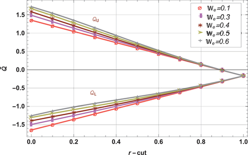
Figure 7. Influence of increasing $\lambda$ on triangular membership function (lifting case) for $\varphi$=2, $X$=1, $W_e$=0.3 and $S_t$ =1.

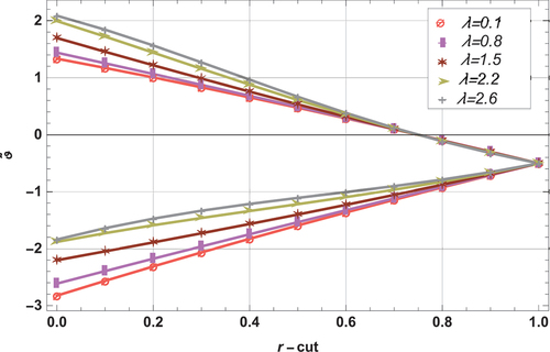
Figure 8. Influence of $\varphi$ on triangular membership function (lifting case) for $\lambda$=0.1, $x$=0.5, $W_e$=1 and $S_t$=0.2.

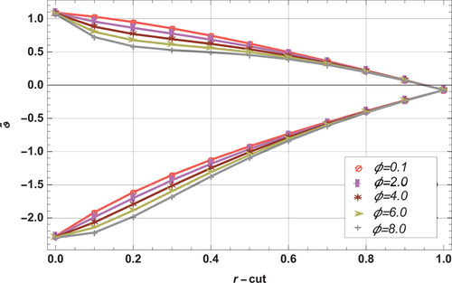
Figure 9. Influence of increasing $W_e$ on flow rate (draining case) when $\varphi$=4, $\lambda =1.3$ and $S_t$=0.5.

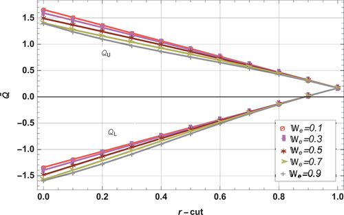
Figure 10. Influence of $\lambda$ on fuzzy velocity profile (draining case) when $r=0.4$, $\varphi$ = 0.03 and $W_e$=0.4.

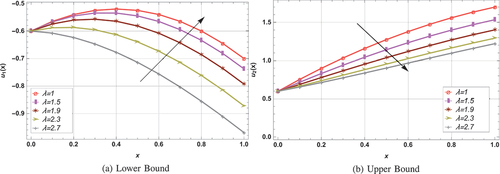
Figure 11. Influence of $S_t$ on fuzzy velocity profile (draining case) when $\lambda$=0.2,$r=0.4$, $\varphi$ = 0.2 and $W_e$=1.0.

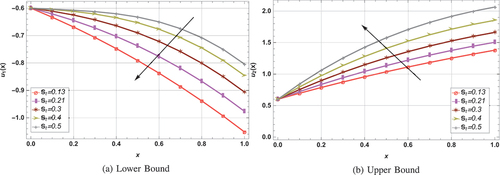
Figure 12. Influence of $W_e$ on fuzzy velocity profile (draining case) when $\lambda$=0.14, $r=0.2$, $\varphi$ = 2 and $S_t$ =0.9.

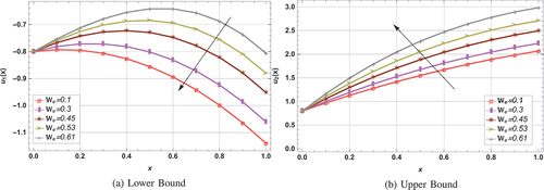
Figure 13. Influence of increasing $\varphi$ on fuzzy velocity profile (draining case) for $r$=0.53, $\lambda =3$ $W_e$=0.98 and $S_t$ =0.65.

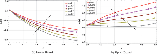
Figure 14. Influence of increasing $\lambda$ on triangular membership function (draining case) for $\varphi$=2, $x$=1, $W_e$=0.3 and $S_t$ =1.

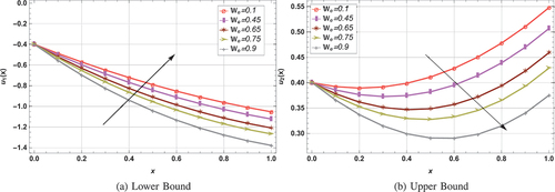
For various fluid and fuzzy parameters, Figures 10–14 illustrate the variations at lower and upper bounds velocity profiles in draining problem. It is noted from Figures 10 and 13 that by increasing the viscosity ratio $\varphi$ and slip parameter $\lambda$, the lower bound velocity profile increases while opposite results are observed at upper bound. It is also seen that upper velocity profile is indirectly while the lower velocity is directly associated with $\varphi$ and $\lambda$. Influence of Stoke’s number $S_t$ and Weissenberg number $W_e$ are depicted in Figures 11 and 12. $S_t$ is used to determine the characterization of fluid particles during experiment. Increase in $S_t$ results in heavier fluid particles by definition, and larger values of $W_e$ corresponds to higher viscous forces between fluid layers. 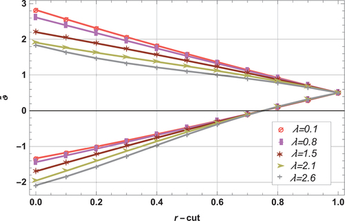As a result velocity of the Jhonson Segalman nanofluid decreases with an increase in $S_t$ and $W_e$ at upper bound, whereas the inverse behavior is recorded at lower bound. In Figure 14, the membership function ($0\le r\le 1$) of fuzzy fluid velocity by increasing $\lambda$ is presented. Variation of $r-cut$ (r = 0.2, 0.25, 0.4, 0.53, 0.51, 0.6 and 0.75) from Figures 3–6 and 10–13 shows that the upper and lower bound fuzzy solutions become closer as $r-cut$ increases from 0 to 1 and will finally result in a crisp solution at $W_e$= 1. In addition, volumetric flow rate at lower and upper bounds for draining problem is depicted in Figure 9. Flow rate decrease at upper bound in drainage case with increase in $W_e$, whereas at lower bound opposite results are recorded.

Figure 3. Influence of $\lambda$ on fuzzy velocity profile (lifting case) when $r=0.75$, ${\mathbb{S}}_t=1$, $\varphi$ = 0.03 and ${\mathbb{W}}_e$ =0.4.

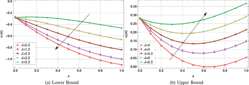
Figure 4. Influence of $\varphi$ on fuzzy velocity profile (lifting case) when $r=0.24$, ${\mathbb{S}}_t=0.2$, $\lambda$ = 0.01 and ${\mathbb{W}}_e$ =1.

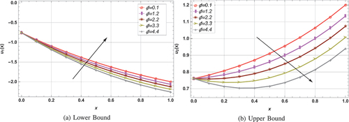
Figure 5. Influence of ${\mathbb{S}}_t$ on fuzzy velocity profile (lifting case) when $\lambda$=0.2,$r$=0.51, $\varphi$ = 0.3 and ${\mathbb{W}}_e$ =1.0.

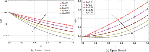
Figure 6. Influence of ${\mathbb{W}}_e$ on fuzzy velocity profile (lifting case) when $\lambda$=0.1,$r$=0.6, $\varphi$ = 4 and ${\mathbb{S}}_t$ =0.5.

Conclusion

The current study focuses on fuzzy modelling of thin film of Jhonson Segalman nanofluid in lifting and drainage cases. To accomplish this, the governing equations were transformed into a system of highly nonlinear fuzzy differential equations by incorporating fuzzified boundary conditions and subsequently solved using the fuzzy modification of the He-Laplace algorithm. Through graphical analysis, the effect of fluid and fuzzy parameters on velocity profiles and volumetric flow rates at upper and lower bounds were examined. Furthermore, the presented methodology was tested (validated) by comparing current results with the existing ones in crisp form. Following are few of the significant findings:

• In lifting case, an indirect relationship is observed between the Weissenberg number $W_e$, Stoke’s number $S_t$, and viscosity ratio $\varphi$ and velocity profile at upper bound. However, at the lower bound opposite behaviour is seen.

• In draining case, increased $\varphi$ and $\lambda$ exhibited direct relationship with velocity at lower bound while opposite behaviour is observced at upper bound.

• For both lifting and drainage scenarios, flow rate decreases as $r$-cut increases.

• Fuzzy solutions converges to crisp solutions when $r$-cut approaches to 1. It demonstrated the consistency and reliability of the obtained fuzzy solutions.

In general, fuzzy modelling provided a better understanding of the physical phenomena, and holds promise for addressing more advanced and complex problems in the fields of science and engineering. Future research will involve analysing the heat and mass transfer in different fluid models.

Disclosure statement

No potential conflict of interest was reported by the author(s).

References

- L.A. Zadeh, Fuzzy sets, Inf. Control 8 (3) (1965), pp. 338–353. doi:10.1016/S0019-9958(65)90241-X.
- I. Beg, R. Noshad Jamil, and T. Rashid, Diminishing choquet hesitant 2-tuple linguistic aggregation operator for multiple attributes group decision making, Inter. J. Anal. Appl 17 (2019), pp. 76–104.
- A. Fahmi, Group decision based on trapezoidal neutrosophic dombi fuzzy hybrid operator, Granul. Comput. 7 (2) (2022), pp. 305–314. doi:10.1007/s41066-021-00268-0.
- M. Rahaman, S. Prasad Mondal, E.A. Algehyne, A. Biswas, and S. Alam, A method for solving linear difference equation in gaussian fuzzy environments, Granul. Comput. 7 (1) (2022), pp. 63–76. doi:10.1007/s41066-020-00251-1.
- M. Ranjbar, S. Effati, and S. Mohsen Miri, Fully hesitant fuzzy linear programming with hesitant fuzzy numbers, Eng. Appl. Artif. Intell. 114 (2022), pp. 105047. doi:10.1016/j.engappai.2022.105047.
- Y. Tansel İç and M. Yurdakul, A new long term (strategic) ranking model for machining center selection decisions based on the review of machining center structural components using triangular fuzzy numbers, Decision Anal. J 4 (2022), pp. 100081. doi:10.1016/j.dajour.2022.100081.
- S.C. Subrat Kumar Jena, V. Mahesh, D. Harursampath, H.M. Sedighi, and H.M. Sedighi, Free vibration of functionally graded beam embedded in winkler-pasternak elastic foundation with geometrical uncertainties using symmetric gaussian fuzzy number, Eur. Phys. J. Plus 137 (3) (2022), pp. 1–18. doi:10.1140/epjp/s13360-022-02607-9.
- S. Seikkala, On the fuzzy initial value problem, Fuzzy Sets Sys 24 (3) (1987), pp. 319–330. doi:10.1016/0165-0114(87)90030-3.
- O. Kaleva, Fuzzy differential equations, Fuzzy Sets Sys 24 (3) (1987), pp. 301–317. doi:10.1016/0165-0114(87)90029-7.
- Y. Wen and R. Jafari, Modeling and Control of Uncertain Nonlinear Systems with Fuzzy Equations and Z-Number, Wiley-IEEE Press, 2019.
- J.J. Nieto, The cauchy problem for continuous fuzzy differential equations, Fuzzy Sets Sys 102 (2) (1999), pp. 259–262. doi:10.1016/S0165-0114(97)00094-8.
- P. Prakash, J.J. Nieto, N. Uthirasamy, and G.S. PRIYA, Solving fuzzy boundary value problem by differential transform method, Neural Parallel Sci. Comput 22 (2014), pp. 59–74.
- M. Najariyan, N. Pariz, and H. Vu, Fuzzy linear singular differential equations under granular differentiability concept, Fuzzy Sets Sys 429 (2022), pp. 169–187. doi:10.1016/j.fss.2021.01.003.
- A. Khastan and J.J. Nieto, A boundary value problem for second order fuzzy differential equations, Nonlinear Anal Theory Methods Appl 72 (9–10) (2010), pp. 3583–3593. doi:10.1016/j.na.2009.12.038.
- M. Jabir Khan, P. Kumam, N. Aedh Alreshidi, N. Shaheen, W. Kumam, Z. Shah, and P. Thounthong, The renewable energy source selection by remoteness index-based VIKOR method for generalized intuitionistic fuzzy soft sets, Symmetry 12 (6) (2020), pp. 977. doi:10.3390/sym12060977.
- M. Qayyum, A. Tahir, and S. Acharya. New solutions of fuzzy-fractional fisher models via optimal he–laplace algorithm, Int. J. Intell. Syst. 2023 (2023), pp. 1–21. doi:10.1155/2023/7084316.
- M. Qayyum, A. Tahir, S. Tauseef Saeed, and A. Akgül, Series-form solutions of generalized fractional-fisher models with uncertainties using hybrid approach in caputo sense, Chaos Soliton. Fract. 172 (2023), pp. 113502. doi:10.1016/j.chaos.2023.113502.
- S. Afzal, M. Qayyum, and G. Chambashi, Heat and mass transfer with entropy optimization in hybrid nanofluid using heat source and velocity slip: A hamilton-crosser approach, Sci Rep. 13 (1) (2023). doi:10.1038/s41598-023-39176-5
- M. Qayyum, S. Afzal, M.R. Ali, M. Sohail, N. Imran, and G. Chambashi, Unsteady hybrid nanofluid (uo2, mwcnts/blood) flow between two rotating stretchable disks with chemical reaction and activation energy under the influence of convective boundaries, Sci Rep. 13 (1) (2023). doi:10.1038/s41598-023-32606-4
- M. Qayyum, S. Afzal, S. Tauseef Saeed, A. Akgül, and M. Bilal Riaz, Unsteady hybrid nanofluid (cu-UO2/blood) with chemical reaction and non-linear thermal radiation through convective boundaries: An application to bio-medicine, Heliyon 9 (6) (2023), pp. e16578. doi:10.1016/j.heliyon.2023.e16578.
- M. Qayyum, M. Bilal Riaz, and S. Afzal, Analysis of blood flow of unsteady carreau-yasuda nanofluid with viscous dissipation and chemical reaction under variable magnetic field, Heliyon 9 (6) (2023), pp. e16522. doi:10.1016/j.heliyon.2023.e16522.
- M. Qayyum, S. Afzal, E. Ahmad, and S. Araci, Fractional modeling of non-newtonian casson fluid between two parallel plates, J. Math 2023 (2023), pp. 1–12. doi:10.1155/2023/5517617.
- M. Nadeem, A. Elmoasry, I. Siddique, F. Jarad, R. Muhammad Zulqarnain, J. Alebraheem, N.S. Elazab, and A.M. Khalil, Study of triangular fuzzy hybrid nanofluids on the natural convection flow and heat transfer between two vertical plates, Comput Intell Neurosci 2021 (2021), pp. 1–15. doi:10.1155/2021/3678335.
- M. Nadeem, I. Siddique, F. Jarad, R. Noshad Jamil, and D. Pamučar, Numerical study of mhd third-grade fluid flow through an inclined channel with ohmic heating under fuzzy environment, Math. Problems Eng 2021 (2021), pp. 1–17. doi:10.1155/2021/9137479.
- I. Siddique, R. Noshad Jamil, M. Nadeem, H. Abd El-Wahed Khalifa, F. Alotaibi, I. Khan, M. Andualem, and A. Jajarmi, Fuzzy analysis for thin-film flow of a third-grade fluid down an inclined plane, Math. Problems Eng 2022 (2022), pp. 1–16. doi:10.1155/2022/3495228.
- M. Nadeem, I. Siddique, R. Ali, N. Alshammari, R. Noshad Jamil, N. Hamadneh, I. Khan, M. Andualem, and A. Majumder, Study of third-grade fluid under the fuzzy environment with couette and poiseuille flows, Math. Problems Eng 2022 (2022), pp. 1–19. doi:10.1155/2022/2458253.
- M. Nadeem, I. Siddique, M. Bilal, and R. Ali, Significance of heat transfer for second-grade fuzzy hybrid nanofluid flow past over a stretching/shrinking riga wedge, AIMS Math. 8 (1) (2022), pp. 295–316. doi: 10.3934/math.2023014.
- R.W. Kolkka, D.S. Malkus, M.G. Hansen, and G.R. Ierley, Spurt phenomena of the johnson-segalman fluid and related models, J Nonnewton Fluid Mech 29 (1988), pp. 303–335. doi:10.1016/0377-0257(88)85059-6.
- M. Kanwal, X. Wang, H. Shahzad, M. Sajid, and C. Yiqi, Mathematical modeling of johnson-segalman fluid in blade coating process, J. Plast. Film Sheet. 37 (4) (2021), pp. 463–489. doi:10.1177/8756087920983551.
- M. Javed, A mathematical framework for peristaltic mechanism of non-newtonian fluid in an elastic heated channel with hall effect, Multidis. Model. Mat Struct 17 (2) (2020), pp. 360–372. doi:10.1108/MMMS-11-2019-0200.
- T. Bodnár and A. Sequeira, Analysis of the shear-thinning viscosity behavior of the johnson–segalman viscoelastic fluids, Fluids 7 (1) (2022), pp. 36. doi:10.3390/fluids7010036.
- M.M. Bhatti, T. Abbas, and M.M. Rashidi, Numerical study of entropy generation with nonlinear thermal radiation on magnetohydrodynamics non-newtonian nanofluid through a porous shrinking sheet, J. Magn 21 (3) (2016), pp. 468–475. doi:10.4283/JMAG.2016.21.3.468.
- M. Rashidi, M. Bhatti, M. Abbas, and M. Ali, Entropy generation on MHD blood flow of nanofluid due to peristaltic waves, Entropy 18 (4) (2016), pp. 117. doi:10.3390/e18040117.
- A. Zeeshan, A. Riaz, F. Alzahrani, A. Moqeet, and A. Ahmadian, Flow analysis of two-layer nano/johnson–segalman fluid in a blood vessel-like tube with complex peristaltic wave, Math. Problems Eng 2022 (2022), pp. 1–18. doi:10.1155/2022/5289401.
- Y. Khan, S. Akram, M. Athar, K. Saeed, T. Muhammad, A. Hussain, M. Imran, and H.A. Alsulaimani, The role of double-diffusion convection and induced magnetic field on peristaltic pumping of a johnson–segalman nanofluid in a non-uniform channel, Nanomaterials 12 (7) (2022), pp. 1051. doi:10.3390/nano12071051.
- C.D. Denson, The drainage of newtonian liquids entrained on a vertical surface, Ind. Eng. Chem. Fund. 9 (3) (1970), pp. 443–448. doi:10.1021/i160035a022.
- A.M. Siddiqui, R. Mahmood, and Q.K. Ghori, Some exact solutions for the thin film flow of a PTT fluid, Phys Lett A 356 (4–5) (2006), pp. 353–356. doi:10.1016/j.physleta.2006.03.071.
- A.M. Siddiqui, R. Mahmood, and Q.K. Ghori, Homotopy perturbation method for thin film flow of a third grade fluid down an inclined plane, Chaos Soliton. Fract. 35 (1) (2008), pp. 140–147. doi:10.1016/j.chaos.2006.05.026.
- S. Ullah, K. Akhtar, N. Alam Khan, and A. Ullah, Analysis of thin film flow of generalized maxwell fluid confronting withdrawal and drainage on non-isothermal cylindrical surfaces, Adv. Mech. Eng 11 (10) (2019), pp. 168781401988100. doi:10.1177/1687814019881005.
- Y. Ruan, A. Nadim, and M. Chugunova, Thin liquid film resulting from a distributed source on a vertical wall, Phys. Rev. Fluids. 5 (6) (2020). doi:10.1103/PhysRevFluids.5.064004
- M.Q. Farnaz, S. Inayat Ali Shah, S.-W. Yao, N. Imran, and M. Sohail, Homotopic fractional analysis of thin film flow of oldroyd 6-constant fluid, Alex. Eng. J. 60 (6) (2021), pp. 5311–5322. doi:10.1016/j.aej.2021.04.036.
- S. Nasir, Z. Shah, S. Islam, E. Bonyah, and T. Gul, Darcy forchheimer nanofluid thin film flow of SWCNTs and heat transfer analysis over an unsteady stretching sheet, AIP Adv. 9 (1) (2019), pp. 015223. doi:10.1063/1.5083972.
- S.A.S. Sehrish, A. Mouldi, and N. Sene, Nonlinear convective SiO2 and TiO2 hybrid nanofluid flow over an inclined stretched surface, null 2022 (2022), pp. 1–11. doi:10.1155/2022/6237698.
- Z. Shah, A. Ullah, E. Bonyah, M. Ayaz, S. Islam, and I. Khan, Hall effect on titania nanofluids thin film flow and radiative thermal behavior with different base fluids on an inclined rotating surface, AIP Adv. 9 (5) (2019), pp. 055113. doi:10.1063/1.5099435.
- S. Ahmed and X. Hang, Mixed convection in gravity-driven thin nano-liquid film flow with homogeneous–heterogeneous reactions, Phys. Fluids 32 (2) (2020), pp. 023604. doi:10.1063/1.5140366.
- Z. Shah, E.O. Alzahrani, A. Dawar, W. Alghamdi, and M. Zaka Ullah, Entropy generation in MHD second-grade nanofluid thin film flow containing CNTs with cattaneo-christov heat flux model past an unsteady stretching sheet, Appl. Sci. 10 (8) (2020), pp. 2720. doi:10.3390/app10082720.
- M. Kamran Alam, M.T. Rahim, T. Haroon, S. Islam, and A.M. Siddiqui, Solution of steady thin film flow of johnson–segalman fluid on a vertical moving belt for lifting and drainage problems using adomian decomposition method, Appl. Math. Comput. 218 (21) (2012), pp. 10413–10428. doi:10.1016/j.amc.2012.03.095.
- M. Madani and M. Fathizadeh, Homotopy perturbation algorithm using laplace transformation, Nonlinear Sci. Lett. A 1 (2010), pp. 263–267.
- M. Qayyum, E. Ahmad, S. Tauseef Saeed, A. Akgül, and M. Bilal Riaz, Traveling wave solutions of generalized seventh-order time-fractional kdv models through he-laplace algorithm, Alex. Eng. J. 70 (2023), pp. 1–11. doi:10.1016/j.aej.2023.02.007.
- H. Ji-Huan, G.M. Moatimid, and D.R. Mostapha, Nonlinear instability of two streaming-superposed magnetic reiner-rivlin fluids by he-laplace method, J. Electroanal. Chem. 895 (2021), pp. 115388. doi:10.1016/j.jelechem.2021.115388.
- B. Hong, J. Wang, and L. Chen, Analytical solutions to a class of fractional coupled nonlinear schrödinger equations via-laplace-hpm technique, AIMS Math 8 (7) (2023), pp. 15670–15688. doi:10.3934/math.2023800.
- N. Gasilov, S.G. Amrahov, and A. Golayoglu Fatullayev, A geometric approach to solve fuzzy linear systems of differential equations, arXiv Preprint arXiv: 0910.4307 (2009).
- M.W. Johnson and D. Segalman, A model for viscoelastic fluid behavior which allows non-affine deformation, J Nonnewton Fluid Mech 2 (3) (1977), pp. 255–270. doi:10.1016/0377-0257(77)80003-7.