Probabilistic degenerate central Bell polynomials

ABSTRACT

Assume that $\mathit{Y}$ is a random variable whose moment generating function exists in a neighbourhood of the origin. In this paper, we study the probabilistic degenerate central Bell polynomials associated with $\mathit{Y}$, as probabilistic extension of the degenerate central Bell polynomials. In addition, we investigate the probabilistic degenerate central factorial numbers of the second kind associated with $\mathit{Y}$ and the probabilistic degenerate central Fubini polynomials associated with $\mathit{Y}$. The aim of this paper is to derive some properties, explicit expressions, certain identities and recurrence relations for those polynomials and numbers.

KEYWORDS:

• Probabilistic degenerate central factorial numbers of the second kind
• probabilistic degenerate central Bell polynomials
• probabilistic degenerate central Fubini polynomials

1. Introduction

It is Carlitz (see Carlitz 1979) who initiated a study of degenerate versions of special polynomials and numbers, namely the degenerate Bernoulli and degenerate Euler polynomials and numbers. In recent years, a lot of work (see Kim et al. 2019, 2019; Kim and Kim 2019, 2022b, 2022a, 2023b; Aydin et al. 2022 and the references therein) has been done regarding various degenerate versions of many special polynomials and numbers. Here, we consider the probabilistic extension of the degenerate central Bell polynomials, which are a degenerate version of the central Bell polynomials. It is fascinating that degenerate gamma fuctions, degenerate umbral calculus and degenerate $\mathit{q}$-umbral calculus have also been developed (see Kim and Kim 2020b, 2021; Kim et al. 2022) during the course of investigations for degenerate versions of some special polynomials and numbers.

Special functions have various importance in a good many areas of engineering, physics, mathematics and other disciplines such as quantum mechanics, mathematical physics, functional analysis, numerical analysis, differential equations and so on. The family of special polynomials possesses also intensive fields of study in the family of special functions. Recently, some probabilistic special polynomials (with their corresponding numbers), including probabilistic Bell, probabilistic Fubini and probabilistic Stirling polynomials (and numbers), are among the most studied families of special polynomials. One of the first papers in this direction was published by Adell and Lekuona (see Adell and Lekuona 2019; Adell 2022). They defined a probabilistic generalization of the Stirling numbers of the second kind and gave some of their properties. We note here that Xu et al. (2024), Withers (2000), Kurt and Simsek (2013), Kim et al. (2019, 2024), Askan et al. (2020) and Kim and Kim (2023a) treat special numbers and polynomials in a probabilistic manner.

Assume that $\mathit{Y}$ is a random variable satisfying the moment condition (see Kim et. al 2024). The aim of this paper is to study, as a probabilistic extension of degenerate central Bell polynomials, the probabilistic degenerate central Bell polynomials associated with $\mathit{Y}$, along with the probabilistic degenerate central factorial numbers of the second kind associated with $\mathit{Y}$ and the probabilistic degenerate central Fubini polynomials associated with $\mathit{Y}$. We derive some properties, explicit expressions, certain identities and recurrence relations for those polynomials and numbers. In addition, we consider the case that $\mathit{Y}$ is the Poisson random variable with parameters $\mathit{\alpha }>0$. Here, we note the following. The central factorial numbers of the second kind appear in the expansion of powers of $\mathit{x}$ in term of central factorials (see Kim and Kim 2020a, 2021, 2023). The degenerate central factorial numbers of the second kind are degenerate versions of the central factorial numbers of the second kind (see Adell and Lekuona 2019). The degenerate central Bell polynomials (see Kim and Kim 2019, 2020a) are natural polynomial extensions of the degenerate central factorial numbers of the second kind.

The outline of this paper is as follows. In Section 1, we recall the Stirling numbers of the second kind, the Stirling numbers of the first kind $\mathit{s}(\mathit{n},\mathit{k})$ together with the table (see Table 1) of $|\mathit{s}(\mathit{n},\mathit{k})|,(0\le \mathit{k}\le \mathit{n}\le 8)$, the degenerate Stirling numbers of the second kind and the degenerate exponentials. We remind the reader of the central factorials, the central factorial numbers of the second kind $\mathit{T}(\mathit{n},\mathit{k})$ together with the table (see Table 2) of $\mathit{T}(\mathit{n},\mathit{k}),(0\le \mathit{k}\le \mathit{n}\le 8)$, the degenerate central factorial numbers of the second kind and the Bell polynomials. Assume that $\mathit{Y}$ is a random variable such that the moment generating function of $\mathit{Y}$, $\mathit{E}[e^{\mathit{tY}}]={\sum }_{n=0}^{\mathrm{\infty }}\frac{t^n}{\mathit{n}!}\mathit{E}[Y^n],(|\mathit{t}|<\mathit{r})$, exists for some $\mathit{r}>0$. Let $(Y_j{)}_{\mathit{j}\ge 1}$ be a sequence of mutually independent copies of the random variable $\mathit{Y}$, and let $S_k=Y_1+Y_2+\cdots +Y_k,(\mathit{k}\ge 1)$, with $S_0=0$. Then, we recall the probabilistic degenerate Stirling numbers of the second kind associated with $\mathit{Y}$, and the probabilistic degenerate Bell polynomials associated with $\mathit{Y}$. We remind the reader of the incomplete Bell polynomials, the complete Bell polynomials, the degenerate Bell polynomials and the degenerate central Bell polynomials. Section 2 contains the main results of this paper. Let $(Y_j{)}_{\mathit{j}\ge 1},S_k,(\mathit{k}=0,1,\dots )$ be as in the above. We define the probabilistic degenerate central factorial numbers of the second kind associated with $\mathit{Y}$, $T_{\lambda }^Y(\mathit{n},\mathit{k})$. In Theorem 1, we get an explicit expression for $T_{\lambda }^Y(\mathit{n},\mathit{k})$. We define the probabilistic degenerate central Bell polynomials associated with $\mathit{Y}$, $C_{n,\lambda }^Y(\mathit{x})$. As to $C_{n,\lambda }^Y(\mathit{x})$, the generating function is found in Theorem 2, and explicit expressions of them are obtained in Theorems 3 and 4. We introduce the probabilistic degenerate central Fubini polynomials associated with $\mathit{Y}$, $W_{n,\lambda }^Y(\mathit{x})$. We derive explicit expressions for $W_{n,\lambda }^Y(\mathit{x})$ in Theorems 5 and 6. We deduce an expression for $T_{\lambda }^Y(\mathit{n},\mathit{k})$ in terms of the incomplete Bell polynomial in Theorem 7 and that for $C_{n,\lambda }^Y(\mathit{x})$ in terms of the Bell polynomial in Theorem 8. A recurrence relation and the convolution formula for $C_{n,\lambda }^Y(\mathit{x})$ are given, respectively, in Theorem 9 and Theorem 10. In Theorem 11, an expression for $C_{n,\lambda }^Y(\mathit{x})$ is obtained in terms of the incomplete Bell polynomials. We get identities involving $T_{\lambda }^Y(\mathit{n},\mathit{k}),C_{n,\lambda }^Y(\mathit{x})$ and the incomplete Bell polynomials in Theorems 12 and 14. The higher-order derivatives of $C_{n,\lambda }^Y(\mathit{x})$ are derived in Theorem 15. Finally, an explicit expression is obtained in Theorem 16 when $\mathit{Y}$ is the Poisson random variable with parameter $\mathit{\alpha }>0$. In Section 3, we illustrate the degenerate central Bell polynomials $C_{\mathit{n},\mathit{\lambda }}(\mathit{x})$ with their graphs. For this, we prove an explicit formula for those polynomials in terms of $\mathit{s}(\mathit{n},\mathit{k})$ and $\mathit{T}(\mathit{n},\mathit{k})$ in Theorem 17. By using Theorem 17 and Tables 1 and 2, we compute $C_{\mathit{n},\mathit{\lambda }}(\mathit{x})$, for $1\le \mathit{n}\le 8$. We plot the graphs of $C_{2,\mathit{\lambda }}(\mathit{x})$, $C_{5,\mathit{\lambda }}(\mathit{x})$, and $C_{8,\mathit{\lambda }}(\mathit{x})$, for the values of $\mathit{\lambda }=1,0.6,0.2$, (see Figure 1). We then conclude the paper in Section 4. As general references on probability and polynomials, the reader may refer to Abramowitz and Stegun (1964), Roman (1984), Leon-Garcia (1994) and Ross (2019). For the rest of this section, we recall the facts that are needed throughout this paper.

Figure 1. The shapes of $C_{\mathit{n},\mathit{\lambda }}(\mathit{x})$.

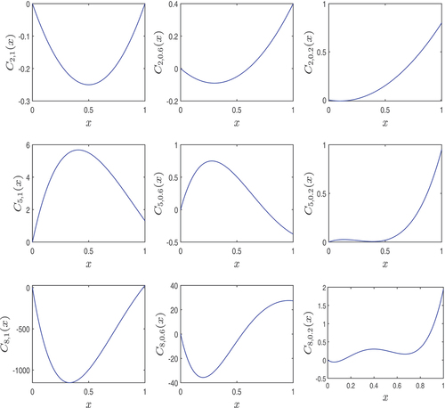
Table 1. |s(n,k)|.

$\mathit{k}$ $\mathit{n}$	0	1	2	3	4	5	6	7	8
0	1
1	0	1
2	0	1	1
3	0	2	3	1
4	0	6	11	6	1
5	0	24	50	35	10	1
6	0	120	274	225	85	15	1
7	0	720	1764	1624	735	175	21	1
8	0	5040	13068	13132	6769	1960	322	28	1

Table 2. T(n,k).

$\mathit{k}$ $\mathit{n}$	0	1	2	3	4	5	6	7	8
0	1
1	0	1
2	0	0	1
3	0	$\frac{1}{4}$	0	1
4	0	0	1	0	1
5	0	$\frac{1}{16}$	0	$\frac{5}{2}$	0	1
6	0	0	1	0	5	0	1
7	0	$\frac{1}{64}$	0	$\frac{91}{16}$	0	$\frac{35}{4}$	0	1
8	0	0	1	0	21	0	14	0	1

For $\mathit{n}\in \mathbb{N}\cup \{0\}$, the Stirling numbers of the second kind are defined by

(1) $x^n=\sum _{\mathit{k}=0}^n\mathit{S}\left(\mathit{n},\mathit{k}\right)(\mathit{x}{)}_k,$(1)

(see Comtet 1974; Roman 1984) where $(\mathit{x}{)}_0=1,(\mathit{x}{)}_n=\mathit{x}(\mathit{x}-1)\cdots (\mathit{x}-(\mathit{n}-1)),(\mathit{n}\ge 1)$.

The Stirling numbers of the first kind are, as the inversion formula of (1), given by

${\left(x\right)}_n=\sum _{\mathit{k}=0}^n\mathit{s}\left(\mathit{n},\mathit{k}\right)x^k$

(see Comtet 1974; Roman 1984) As is well known, the generating function of the Stirling numbers of the first kind is given by

(2) $\frac{1}{\mathit{k}!}(log(1+\mathit{t}){)}^k=\sum _{\mathit{n}=\mathit{k}}^{\mathrm{\infty }}\mathit{s}(\mathit{n},\mathit{k})\frac{t^n}{\mathit{n}!}.$(2)

The Stirling numbers of the first kind satisfy the following recurrence relation together with the initial conditions (see Roman 1984, p.61):

(3) $\mathit{s}(\mathit{n}+1,\mathit{k})=\mathit{s}(\mathit{n},\mathit{k}-1)-\mathit{ns}(\mathit{n},\mathit{k}),\mathit{s}(0,0)=1,\mathit{s}(\mathit{n},0)=0,(\mathit{n}\ge 1).$(3)

For later use in Section 3, we provide the table for $|\mathit{s}(\mathit{n},\mathit{k})|$, for $0\le \mathit{k}\le \mathit{n}\le 8$,(see Table 1), which can be computed from the recurrence relation for $\mathit{s}(\mathit{n},\mathit{k})$ in (3).

Let $\mathit{\lambda }$ be any nonzero real number. The degenerate falling factorial sequence (see Kim et al. 2019) is given by

(4) $(\mathit{x}{)}_{0,\mathit{\lambda }}=1,(\mathit{x}{)}_{\mathit{n},\mathit{\lambda }}=\mathit{x}(\mathit{x}-\mathit{\lambda })(\mathit{x}-2\mathit{\lambda })\cdots (\mathit{x}-(\mathit{n}-1)\mathit{\lambda }),(\mathit{n}\ge 1).$(4)

In addition, the degenerate rising factorial sequence (see Kim et al. 2019) is defined by

(5) $⟨\mathit{x}{⟩}_{0,\mathit{\lambda }}=1,⟨\mathit{x}{⟩}_{\mathit{n},\mathit{\lambda }}=\mathit{x}(\mathit{x}+\mathit{\lambda })(\mathit{x}+2\mathit{\lambda })\cdots (\mathit{x}+(\mathit{n}-1)\mathit{\lambda }),(\mathit{n}\ge 1).$(5)

The two degenerate factorial sequences are related to each other as in the following:

(6) ${\left(-\mathit{x}\right)}_{\mathit{n},\mathit{\lambda }}=(-1{)}^n(\mathit{x}){ }_{\mathit{n},\mathit{\lambda }},⟨-\mathit{x}⟩{ }_{\mathit{n},\mathit{\lambda }}=(-1{)}^n{\left(x\right)}_{\mathit{n},\mathit{\lambda }},$(6)

(see Kim and Kim 2022b). The degenerate Stirling numbers of the second kind are defined by Kim–Kim as

(7) ${\left(x\right)}_{\mathit{n},\mathit{\lambda }}=\sum _{\mathit{k}=0}^n{S}_{\lambda }\left(\mathit{n},\mathit{k}\right)(\mathit{x}{)}_k,\left(\mathit{n}\ge 0\right),$(7)

(see Kim and Kim 2022b, 2022a, 2023b). Note that ${lim}_{\mathit{\lambda }\to 0}{S}_{\lambda }(\mathit{n},\mathit{k})=\mathit{S}(\mathit{n},\mathit{k}),(\mathit{n}\ge \mathit{k}\ge 0)$.

The degenerate exponentials are given by

(8) $e_{\lambda }^x\left(\mathit{t}\right)=(1+\mathit{\lambda t}{)}^{\frac{x}{\lambda }}=\sum _{\mathit{n}=0}^{\mathrm{\infty }}{\left(x\right)}_{\mathit{n},\mathit{\lambda }}\frac{t^n}{\mathit{n}!},e_{\lambda }\left(\mathit{t}\right)=e_{\lambda }^1\left(\mathit{t}\right),$(8)

(see Kim et al. 2019, 2019; Kim and Kim 2019, 2022b, 2022a, 2023b). The central factorials $x^{[\mathit{n}]}$ (see Kim et al. 2019; Kim and Kim 2019, 2020a, 2023) are defined by

(9) $x^{[0]}=1,x^{[\mathit{n}]}=\mathit{x}(\mathit{x}+\frac{n}{2}-1)(\mathit{x}+\frac{n}{2}-2)\cdots (\mathit{x}+\frac{n}{2}-\mathit{n}+1),(\mathit{n}\ge 1).$(9)

The central factorial numbers of the second kind are defined by

(10) $x^n=\sum _{\mathit{k}=0}^n\mathit{T}\left(\mathit{n},\mathit{k}\right)x^{\left[\mathit{k}\right]},\left(\mathit{n}\ge 0\right),$(10)

(see Comtet 1974; Kim and Kim 2019, 2020a, 2023; Jang and Kim 2019) We recall the closed-form formulas for $\mathit{T}(\mathit{n},\mathit{k})$ from (Butzer et al. 1989). For nonnegative integers $\mathit{n},\mathit{k}$ with $\mathit{n}\ge \mathit{k}$, we have

(11) $\mathit{T}(\mathit{n},\mathit{k})=(-1{)}^k\sum _{\mathit{j}=\mathit{k}}^n(-1{)}^j\left(\begin{array}{c}\mathit{n}\\ \mathit{j}\end{array}\right){\left(\frac{k}{2}\right)}^{\mathit{n}-\mathit{j}}\mathit{S}(\mathit{j},\mathit{k}),$(11)

(see equation (7.6) of Proposition 7.4 in (Butzer et al. 1989), p.481),

(12) $=\frac{1}{\mathit{k}!}\sum _{\mathit{j}=0}^k(-1{)}^j\left(\begin{array}{c}\mathit{k}\\ \mathit{j}\end{array}\right){\left(\frac{k}{2}-\mathit{j}\right)}^{\mathit{n}}$(12)

(see the equation (xii) of Proposition 2.4 in (Butzer et al. 1989), p.429).

For later use in Section 3, we provide the table for $\mathit{T}(\mathit{n},\mathit{k})$, for $0\le \mathit{k}\le \mathit{n}\le 8$, (see Table 2), which can be computed from the closed-form formulas in Equations (11)(11) $\mathit{T}(\mathit{n},\mathit{k})=(-1{)}^k\sum _{\mathit{j}=\mathit{k}}^n(-1{)}^j\left(\begin{array}{c}\mathit{n}\\ \mathit{j}\end{array}\right){\left(\frac{k}{2}\right)}^{\mathit{n}-\mathit{j}}\mathit{S}(\mathit{j},\mathit{k}),$(11) or (12).

Recently, Kim–Kim introduced the degenerate central factorial numbers of the second kind which are defined by

(13) ${\left(x\right)}_{\mathit{n},\mathit{\lambda }}=\sum _{\mathit{k}=0}^n{T}_{\lambda }\left(\mathit{n},\mathit{k}\right)x^{\left[\mathit{k}\right]},\left(\mathit{n}\ge 0\right),$(13)

(see Kim et al. 2019; Kim and Kim 2019, 2023). From Equation (13)(13) ${\left(x\right)}_{\mathit{n},\mathit{\lambda }}=\sum _{\mathit{k}=0}^n{T}_{\lambda }\left(\mathit{n},\mathit{k}\right)x^{\left[\mathit{k}\right]},\left(\mathit{n}\ge 0\right),$(13) , we have

(14) $\frac{1}{\mathit{k}!}(e_{\lambda }^{12}(\mathit{t})-e_{\lambda }^{-12}(\mathit{t}){)}^k=\sum _{\mathit{n}=\mathit{k}}^{\mathrm{\infty }}{T}_{\lambda }(\mathit{n},\mathit{k})\frac{t^n}{\mathit{n}!},(\mathit{k}\ge 0).$(14)

Observe that, by taking $\mathit{\lambda }\to 0$ in Equation (14)(14) $\frac{1}{\mathit{k}!}(e_{\lambda }^{12}(\mathit{t})-e_{\lambda }^{-12}(\mathit{t}){)}^k=\sum _{\mathit{n}=\mathit{k}}^{\mathrm{\infty }}{T}_{\lambda }(\mathit{n},\mathit{k})\frac{t^n}{\mathit{n}!},(\mathit{k}\ge 0).$(14) , we have the generating function of the central factorial numbers $\mathit{T}(\mathit{n},\mathit{k})$:

(15) $\frac{1}{\mathit{k}!}(e^{\frac{t}{2}}-e^{-\frac{t}{2}}{)}^k=\sum _{\mathit{n}=\mathit{k}}^{\mathrm{\infty }}\mathit{T}(\mathit{n},\mathit{k})\frac{t^n}{\mathit{n}!}.$(15)

It is well known that the Bell polynomials are given by

(16) $e^{x\left(e^t-1\right)}=\sum _{\mathit{n}=0}^{\mathrm{\infty }}{\text{phii}}_n\left(\mathit{x}\right)\frac{t^n}{\mathit{n}!},$(16)

(see Comtet 1974; Roman 1984; Abbas and Bouroubi 2005; Kim and Kim 2023a). Assume that $\mathit{Y}$ is a random variable whose moment generating function exists in a neighbourhood of the origin, i.e.

(17) $\mathit{E}[e^{\mathit{tY}}]=\sum _{\mathit{n}=0}^{\mathrm{\infty }}\frac{E[Y^n]}{\mathit{n}!}{t}^n,(|\mathit{t}|<\mathit{r}),\mathrm{exists}\mathrm{for}\mathrm{some}\mathit{r}>0.$(17)

Let $(Y_j{)}_{\mathit{j}\ge 1}$ be a sequence of mutually independent copies of the random variable $\mathit{Y}$, and let

(18) $S_0=0,S_k=Y_1+Y_2+\cdots +Y_k,(\mathit{k}\ge 1).$(18)

Then the probabilistic degenerate Stirling numbers of the second kind associated with $\mathit{Y}$ are given by

(19) $S_{\mathit{Y},\mathit{\lambda }}(\mathit{n},\mathit{k})=\frac{1}{\mathit{k}!}\sum _{\mathit{j}=0}^k\left(\begin{array}{c}\mathit{k}\\ \mathit{j}\end{array}\right)(-1{)}^{\mathit{k}-\mathit{j}}\mathit{E}[(S_j{)}_{\mathit{n},\mathit{\lambda }}],$(19)

where $\mathit{n}\ge \mathit{k}\ge 0$, (see Kim and Kim 2023a; Kim et al. 2024).

In Kim and Kim (2023a), the probabilistic degenerate Bell polynomials associated with $\mathit{Y}$ are defined by

(20) ${\text{phii}}_{n,\lambda }^Y(\mathit{x})=\sum _{\mathit{k}=0}^n{S}_{\mathit{Y},\mathit{\lambda }}(\mathit{n},\mathit{k})x^k,(\mathit{n}\ge 0).$(20)

From Equations (19)(19) $S_{\mathit{Y},\mathit{\lambda }}(\mathit{n},\mathit{k})=\frac{1}{\mathit{k}!}\sum _{\mathit{j}=0}^k\left(\begin{array}{c}\mathit{k}\\ \mathit{j}\end{array}\right)(-1{)}^{\mathit{k}-\mathit{j}}\mathit{E}[(S_j{)}_{\mathit{n},\mathit{\lambda }}],$(19) and (20), we note that

(21) $\frac{1}{\mathit{k}!}(\mathit{E}[e_{\lambda }^Y(\mathit{t})]-1{)}^k=\sum _{\mathit{n}=\mathit{k}}^{\mathrm{\infty }}{S}_{\mathit{Y},\mathit{\lambda }}(\mathit{n},\mathit{k})\frac{t^n}{\mathit{n}!},(\mathit{k}\ge 0),$(21)

and

(22) $e^{x(E[e_{\lambda }^Y(\mathit{t})]-1)}=\sum _{\mathit{n}=0}^{\mathrm{\infty }}{\text{phii}}_{n,\lambda }^Y(\mathit{x})\frac{t^n}{\mathit{n}!},(\mathrm{see}[16]),$(22)

where we note that

(23) $\mathit{E}[e_{\lambda }^Y(\mathit{t})]=\sum _{\mathit{n}=0}^{\mathrm{\infty }}\mathit{E}[(\mathit{Y}{)}_{\mathit{n},\mathit{\lambda }}]\frac{t^n}{\mathit{n}!}.$(23)

Let $\mathit{k}$ be a nonnegative integer. The incomplete Bell polynomials are defined by

(24) $\frac{1}{\mathit{k}!}{\left(\sum _{\mathit{m}=1}^{\mathrm{\infty }}{x}_m\frac{t^m}{\mathit{m}!}\right)}^{\mathit{k}}=\sum _{\mathit{n}=\mathit{k}}^{\mathrm{\infty }}{B}_{\mathit{n},\mathit{k}}\left(x_1,x_2,\dots ,x_{\mathit{n}-\mathit{k}+1}\right)\frac{t^n}{\mathit{n}!},$(24)

(see Comtet 1974; Kim and Kim 2023a). From Equation (24)(24) $\frac{1}{\mathit{k}!}{\left(\sum _{\mathit{m}=1}^{\mathrm{\infty }}{x}_m\frac{t^m}{\mathit{m}!}\right)}^{\mathit{k}}=\sum _{\mathit{n}=\mathit{k}}^{\mathrm{\infty }}{B}_{\mathit{n},\mathit{k}}\left(x_1,x_2,\dots ,x_{\mathit{n}-\mathit{k}+1}\right)\frac{t^n}{\mathit{n}!},$(24) , we see that the incomplete Bell polynomials are explicitly given by

(25) $\begin{array}{cc}& B_{\mathit{n},\mathit{k}}(x_1,x_2,\dots ,x_{\mathit{n}-\mathit{k}+1})\\ \mathit{\hspace{0.17em}}& \begin{array}{c}=\sum _{\genfrac{}{}{0ex}{}{l_1+l_2+\cdots +l_{\mathit{n}-\mathit{k}+1}=\mathit{k}}{l_1+2l_2+\cdots +(\mathit{n}-\mathit{k}+1)l_{\mathit{n}-\mathit{k}+1}=\mathit{n}}}\frac{\mathit{n}!}{l_1!l_2!\cdots l_{\mathit{n}-\mathit{k}+1}!}(\frac{x_1}{1!}{)}^{l_1}(\frac{x_2}{2!}{)}^{l_2}\cdots (\frac{{\mathit{x}}_{\mathit{n}-\mathit{k}+1}}{(\mathit{n}-\mathit{k}+1)!}{)}^{{\mathit{l}}_{\mathit{n}-\mathit{k}+1}}.\end{array}\end{array}$(25)

The complete Bell polynomials are given by

(26) $e^{\sum _{\mathit{i}=1}^{\mathrm{\infty }}{x}_i\frac{t^i}{\mathit{i}!}}=\sum _{\mathit{n}=0}^{\mathrm{\infty }}{B}_n\left(x_1,x_2,\dots ,x_n\right)\frac{t^n}{\mathit{n}!},$(26)

(see Comtet 1974; Kim and Kim 2023a). By Equations (25)(25) $\begin{array}{cc}& B_{\mathit{n},\mathit{k}}(x_1,x_2,\dots ,x_{\mathit{n}-\mathit{k}+1})\\ \mathit{\hspace{0.17em}}& \begin{array}{c}=\sum _{\genfrac{}{}{0ex}{}{l_1+l_2+\cdots +l_{\mathit{n}-\mathit{k}+1}=\mathit{k}}{l_1+2l_2+\cdots +(\mathit{n}-\mathit{k}+1)l_{\mathit{n}-\mathit{k}+1}=\mathit{n}}}\frac{\mathit{n}!}{l_1!l_2!\cdots l_{\mathit{n}-\mathit{k}+1}!}(\frac{x_1}{1!}{)}^{l_1}(\frac{x_2}{2!}{)}^{l_2}\cdots (\frac{{\mathit{x}}_{\mathit{n}-\mathit{k}+1}}{(\mathit{n}-\mathit{k}+1)!}{)}^{{\mathit{l}}_{\mathit{n}-\mathit{k}+1}}.\end{array}\end{array}$(25) and (26), we get

(27) $B_n(x_1,x_2,\dots ,x_n)=\sum _{\mathit{k}=0}^n{B}_{\mathit{n},\mathit{k}}(x_1,x_2,\dots ,x_{\mathit{n}-\mathit{k}+1}).$(27)

Note that

(28) $B_{\mathit{n},\mathit{k}}((1{)}_{1,\mathit{\lambda }},(1{)}_{2,\mathit{\lambda }},(1{)}_{3,\mathit{\lambda }},\dots ,(1{)}_{\mathit{n}-\mathit{k}+1,\mathit{\lambda }})=S_{\lambda }(\mathit{n},\mathit{k}),(\mathit{n}\ge \mathit{k}\ge 0),$(28)

and

(29) $B_n(\mathit{x}(1{)}_{1,\mathit{\lambda }},\mathit{x}(1{)}_{2,\mathit{\lambda }},\dots ,\mathit{x}(1{)}_{\mathit{n},\mathit{\lambda }})={\text{phii}}_{\mathit{n},\mathit{\lambda }}(\mathit{x}),(\mathit{n}\ge 0),$(29)

(see (24),(26)),

where ${\text{phii}}_{\mathit{n},\mathit{\lambda }}(\mathit{x})$ are the degenerate Bell polynomials (see Kim et al. 2019; Kim and Kim 2022a) given by

$\sum _{\mathit{k}=0}^n{S}_{\lambda }(\mathit{n},\mathit{k})x^k.$

In Kim and Kim (2019), the degenerate central Bell polynomials are given by

(30) $e^{x(e_{\lambda }^{12}(\mathit{t})-e_{\lambda }^{-12}(\mathit{t}))}=\sum _{\mathit{n}=0}^{\mathrm{\infty }}{C}_{\mathit{n},\mathit{\lambda }}(\mathit{x})\frac{t^n}{\mathit{n}!}.$(30)

Thus, by (14) and (30), we get

(31) $C_{\mathit{n},\mathit{\lambda }}(\mathit{x})=\sum _{\mathit{k}=0}^n{T}_{\lambda }(\mathit{n},\mathit{k})x^k,(\mathit{n}\ge 0).$(31)

2. Probabilistic degenerate central Bell polynomials

Let $\mathit{Y}$ be a random variable, and let $(Y_j{)}_{\mathit{j}\ge 1}$ be a sequence of mutually independent copies of the random variable $\mathit{Y}$ with

(32) $S_0=0,S_k=Y_1+Y_2+\cdots +Y_k,(\mathit{k}\ge 1).$(32)

We define the probabilistic degenerate central factorial numbers of the second kind associated with $\mathit{Y}$ by

(33) $\frac{1}{\mathit{k}!}(\mathit{E}[e_{\lambda }^{\frac{Y}{2}}(\mathit{t})]-\mathit{E}[e_{\lambda }^{-\frac{Y}{2}}(\mathit{t})]{)}^k=\sum _{\mathit{n}=\mathit{k}}^{\mathrm{\infty }}{T}_{\lambda }^Y(\mathit{n},\mathit{k})\frac{t^n}{\mathit{n}!},(\mathit{k}\ge 0).$(33)

When $\mathit{Y}=1$, $T_{\lambda }^1(\mathit{n},\mathit{k})=T_{\lambda }(\mathit{n},\mathit{k}),(\mathit{n}\ge \mathit{k}\ge 0)$. Hereafter, ‘$\mathit{Y}=1$’ means $\mathit{Y}$ is the discrete random variable that takes on the only value 1.

From Equation (33)(33) $\frac{1}{\mathit{k}!}(\mathit{E}[e_{\lambda }^{\frac{Y}{2}}(\mathit{t})]-\mathit{E}[e_{\lambda }^{-\frac{Y}{2}}(\mathit{t})]{)}^k=\sum _{\mathit{n}=\mathit{k}}^{\mathrm{\infty }}{T}_{\lambda }^Y(\mathit{n},\mathit{k})\frac{t^n}{\mathit{n}!},(\mathit{k}\ge 0).$(33) , we have

(34) ${\displaystyle \sum _{\mathit{n}=\mathit{k}}^{\infty }{T}_{\lambda }^Y}(\mathit{n},\mathit{k})\frac{t^n}{\mathit{n}!}=\frac{1}{\mathit{k}!}{(E[e_{\lambda }^{\frac{Y}{2}}(\mathit{t})]-\mathit{E}[e_{\lambda }^{-\frac{Y}{2}}(\mathit{t})])}^{\mathit{k}}=\frac{1}{\mathit{k}!}{\displaystyle \sum _{\mathit{j}=0}^k\left(\mathit{k}\mathit{j}\right)}{(-1)}^{\mathit{k}-\mathit{j}}{\left(E[e_{\lambda }^{\frac{Y}{2}}(\mathit{t})]\right)}^{\mathit{j}}{\left(E[e_{\lambda }^{-\frac{Y}{2}}(\mathit{t})]\right)}^{\mathit{k}-\mathit{j}}=\frac{1}{\mathit{k}!}{\displaystyle \sum _{\mathit{j}=0}^k\left(\mathit{k}\mathit{j}\right)}{(-1)}^{\mathit{k}-\mathit{j}}\mathit{E}[e_{\lambda }^{\frac{S_j}{2}}(\mathit{t})]\mathit{E}[e_{\lambda }^{-\frac{{\mathit{S}}_{\mathit{k}-\mathit{j}}}{2}}(\mathit{t})]=\frac{1}{\mathit{k}!}{\displaystyle \sum _{\mathit{j}=0}^k\left(\mathit{kj}\right)}{(-1)}^{\mathit{k}-\mathit{j}}{\displaystyle \sum _{\mathit{n}=0}^{\infty }{\displaystyle \sum }_{\mathit{l}=0}^n}\left(\mathit{nl}\right)E{\left(\frac{S_j}{2}\right)}_{\mathit{l},\mathit{\lambda }}{(-1)}^{\mathit{n}-\mathit{l}}\mathit{E}\left[{〈\frac{{\mathit{S}}_{\mathit{k}-\mathit{j}}}{2}〉}_{\mathit{n}-\mathit{l},\mathit{\lambda }}\right]\frac{t^n}{\mathit{n}!}={\displaystyle \sum _{\mathit{n}=0}^{\infty }\frac{1}{\mathit{k}!}}{\displaystyle \sum _{\mathit{j}=0}^k{\displaystyle \sum _{\mathit{l}=0}^n\left(\mathit{n}\mathit{l}\right)}}\left(\mathit{k}\mathit{j}\right){(-1)}^{\mathit{n}-\mathit{k}-\mathit{l}-\mathit{j}}\mathit{E}{\left(\frac{S_j}{2}\right)}_{\mathit{l},\mathit{\lambda }}\mathit{E}\left[{〈\frac{{\mathit{S}}_{\mathit{k}-\mathit{j}}}{2}〉}_{\mathit{n}-\mathit{l},\mathit{\lambda }}\right]\frac{t^n}{\mathit{n}!}.$(34)

Here the third line follows from the second by using the assumption that $(Y_j{)}_{\mathit{j}\ge 1}$ is a sequence of mutually independent copies of $\mathit{Y}$ and the fourth line from the third by utilizing Equation (23)(23) $\mathit{E}[e_{\lambda }^Y(\mathit{t})]=\sum _{\mathit{n}=0}^{\mathrm{\infty }}\mathit{E}[(\mathit{Y}{)}_{\mathit{n},\mathit{\lambda }}]\frac{t^n}{\mathit{n}!}.$(23) .

Therefore, by comparing the coefficients on both sides of Equation (34)(34) ${\displaystyle \sum _{\mathit{n}=\mathit{k}}^{\infty }{T}_{\lambda }^Y}(\mathit{n},\mathit{k})\frac{t^n}{\mathit{n}!}=\frac{1}{\mathit{k}!}{(E[e_{\lambda }^{\frac{Y}{2}}(\mathit{t})]-\mathit{E}[e_{\lambda }^{-\frac{Y}{2}}(\mathit{t})])}^{\mathit{k}}=\frac{1}{\mathit{k}!}{\displaystyle \sum _{\mathit{j}=0}^k\left(\mathit{k}\mathit{j}\right)}{(-1)}^{\mathit{k}-\mathit{j}}{\left(E[e_{\lambda }^{\frac{Y}{2}}(\mathit{t})]\right)}^{\mathit{j}}{\left(E[e_{\lambda }^{-\frac{Y}{2}}(\mathit{t})]\right)}^{\mathit{k}-\mathit{j}}=\frac{1}{\mathit{k}!}{\displaystyle \sum _{\mathit{j}=0}^k\left(\mathit{k}\mathit{j}\right)}{(-1)}^{\mathit{k}-\mathit{j}}\mathit{E}[e_{\lambda }^{\frac{S_j}{2}}(\mathit{t})]\mathit{E}[e_{\lambda }^{-\frac{{\mathit{S}}_{\mathit{k}-\mathit{j}}}{2}}(\mathit{t})]=\frac{1}{\mathit{k}!}{\displaystyle \sum _{\mathit{j}=0}^k\left(\mathit{kj}\right)}{(-1)}^{\mathit{k}-\mathit{j}}{\displaystyle \sum _{\mathit{n}=0}^{\infty }{\displaystyle \sum }_{\mathit{l}=0}^n}\left(\mathit{nl}\right)E{\left(\frac{S_j}{2}\right)}_{\mathit{l},\mathit{\lambda }}{(-1)}^{\mathit{n}-\mathit{l}}\mathit{E}\left[{〈\frac{{\mathit{S}}_{\mathit{k}-\mathit{j}}}{2}〉}_{\mathit{n}-\mathit{l},\mathit{\lambda }}\right]\frac{t^n}{\mathit{n}!}={\displaystyle \sum _{\mathit{n}=0}^{\infty }\frac{1}{\mathit{k}!}}{\displaystyle \sum _{\mathit{j}=0}^k{\displaystyle \sum _{\mathit{l}=0}^n\left(\mathit{n}\mathit{l}\right)}}\left(\mathit{k}\mathit{j}\right){(-1)}^{\mathit{n}-\mathit{k}-\mathit{l}-\mathit{j}}\mathit{E}{\left(\frac{S_j}{2}\right)}_{\mathit{l},\mathit{\lambda }}\mathit{E}\left[{〈\frac{{\mathit{S}}_{\mathit{k}-\mathit{j}}}{2}〉}_{\mathit{n}-\mathit{l},\mathit{\lambda }}\right]\frac{t^n}{\mathit{n}!}.$(34) , we obtain the following theorem.

Theorem 1.

For $\mathit{n}\ge \mathit{k}\ge 0$, we have

$T_{\lambda }^Y(\mathit{n},\mathit{k})=\frac{1}{\mathit{k}!}{\displaystyle \sum _{\mathit{j}=0}^k{\displaystyle \sum _{\mathit{l}=0}^n\left(\mathit{n}\mathit{l}\right)}}\left(\mathit{k}\mathit{j}\right){(-1)}^{\mathit{n}-\mathit{k}-\mathit{l}-\mathit{j}}\mathit{E}{\left(\frac{S_j}{2}\right)}_{\mathit{l},\mathit{\lambda }}\mathit{E}\left[{〈\frac{{\mathit{S}}_{\mathit{k}-\mathit{j}}}{2}〉}_{\mathit{n}-\mathit{l},\mathit{\lambda }}\right].$

In view of Equation (31)(31) $C_{\mathit{n},\mathit{\lambda }}(\mathit{x})=\sum _{\mathit{k}=0}^n{T}_{\lambda }(\mathit{n},\mathit{k})x^k,(\mathit{n}\ge 0).$(31) , we define the probabilistic degenerate central Bell polynomials associated with $\mathit{Y}$ by

(35) $C_{n,\lambda }^Y(\mathit{x})=\sum _{\mathit{k}=0}^n{T}_{\lambda }^Y(\mathit{n},\mathit{k})x^k,(\mathit{n}\ge 0).$(35)

Especially, $C_{n,\lambda }^Y=C_{n,\lambda }^Y(1),(\mathit{n}\ge 0)$, are called the probabilistic degenerate central Bell numbers associated with $\mathit{Y}$. When $\mathit{Y}=1$, $C_{n,\lambda }^1(\mathit{x})=C_{\mathit{n},\mathit{\lambda }}(\mathit{x})$. From Equations (35)(35) $C_{n,\lambda }^Y(\mathit{x})=\sum _{\mathit{k}=0}^n{T}_{\lambda }^Y(\mathit{n},\mathit{k})x^k,(\mathit{n}\ge 0).$(35) and (33), we note that

(36) $\begin{array}{rl}& \sum _{\mathit{n}=0}^{\mathrm{\infty }}{C}_{n,\lambda }^Y(\mathit{x})\frac{t^n}{\mathit{n}!}=\sum _{\mathit{n}=0}^{\mathrm{\infty }}\sum _{\mathit{k}=0}^n{T}_{\lambda }^Y(\mathit{n},\mathit{k})x^k\frac{t^n}{\mathit{n}!}=\sum _{\mathit{k}=0}^{\mathrm{\infty }}\sum _{\mathit{n}=\mathit{k}}^{\mathrm{\infty }}{T}_{\lambda }^Y(\mathit{n},\mathit{k})\frac{t^n}{\mathit{n}!}{x}^k\\ & =\sum _{\mathit{n}=0}^{\mathrm{\infty }}\frac{x^k}{\mathit{k}!}(\mathit{E}[e_{\lambda }^{\frac{Y}{2}}(\mathit{t})]-\mathit{E}[e_{\lambda }^{-\frac{Y}{2}}(\mathit{t})]{)}^k\\ & =e^{x(E[e_{\lambda }^{\frac{Y}{2}}(\mathit{t})]-\mathit{E}[e_{\lambda }^{-\frac{Y}{2}}(\mathit{t})])}.\end{array}$(36)

Therefore, by Equation (36)(36) $\begin{array}{rl}& \sum _{\mathit{n}=0}^{\mathrm{\infty }}{C}_{n,\lambda }^Y(\mathit{x})\frac{t^n}{\mathit{n}!}=\sum _{\mathit{n}=0}^{\mathrm{\infty }}\sum _{\mathit{k}=0}^n{T}_{\lambda }^Y(\mathit{n},\mathit{k})x^k\frac{t^n}{\mathit{n}!}=\sum _{\mathit{k}=0}^{\mathrm{\infty }}\sum _{\mathit{n}=\mathit{k}}^{\mathrm{\infty }}{T}_{\lambda }^Y(\mathit{n},\mathit{k})\frac{t^n}{\mathit{n}!}{x}^k\\ & =\sum _{\mathit{n}=0}^{\mathrm{\infty }}\frac{x^k}{\mathit{k}!}(\mathit{E}[e_{\lambda }^{\frac{Y}{2}}(\mathit{t})]-\mathit{E}[e_{\lambda }^{-\frac{Y}{2}}(\mathit{t})]{)}^k\\ & =e^{x(E[e_{\lambda }^{\frac{Y}{2}}(\mathit{t})]-\mathit{E}[e_{\lambda }^{-\frac{Y}{2}}(\mathit{t})])}.\end{array}$(36) , we obtain the following theorem.

Theorem 2.

The generating function of the probabilistic degenerate central Bell polynomials associated with $\mathit{Y}$ is given by

(37) $e^{x(E[e_{\lambda }^{\frac{Y}{2}}(\mathit{t})]-\mathit{E}[e_{\lambda }^{-\frac{Y}{2}}(\mathit{t})])}=\sum _{\mathit{n}=0}^{\mathrm{\infty }}{C}_{n,\lambda }^Y(\mathit{x})\frac{t^n}{\mathit{n}!}.$(37)

From Equation (37)(37) $e^{x(E[e_{\lambda }^{\frac{Y}{2}}(\mathit{t})]-\mathit{E}[e_{\lambda }^{-\frac{Y}{2}}(\mathit{t})])}=\sum _{\mathit{n}=0}^{\mathrm{\infty }}{C}_{n,\lambda }^Y(\mathit{x})\frac{t^n}{\mathit{n}!}.$(37) , we note that

(38) ${\displaystyle \sum _{\mathit{n}=0}^{\infty }{C}_{n,\lambda }^Y}(\mathit{x})\frac{t^n}{\mathit{n}!}=e^{x(E[e_{\lambda }^{\frac{Y}{2}}(\mathit{t})])}{e}^{-x(E[e_{\lambda }^{-\frac{Y}{2}}(\mathit{t})])}={\displaystyle \sum _{\mathit{l}=0}^{\infty }\frac{x^l}{\mathit{l}!}}\mathit{E}[e_{\lambda }^{\frac{S_l}{2}}(\mathit{t})]{\displaystyle \sum _{\mathit{j}=0}^{\infty }{(-1)}^j}\frac{x^j}{\mathit{j}!}\mathit{E}[e_{\lambda }^{-\frac{S_j}{2}}(\mathit{t})]={\displaystyle \sum _{\mathit{l}=0}^{\infty }\frac{x^l}{\mathit{l}!}}{\displaystyle \sum _{\mathit{m}=0}^{\infty }\mathit{E}}{S}_{l}2\mathit{m},\mathit{\lambda }\frac{t^m}{\mathit{m}!}{\displaystyle \sum _{\mathit{j}=0}^{\infty }\frac{{(-1)}^j}{\mathit{j}!}}{x}^j{\displaystyle \sum _{\mathit{p}=0}^{\infty }\mathit{E}}{\left(-\frac{S_j}{2}\right)}_{\mathit{p},\mathit{\lambda }}\frac{t^p}{\mathit{p}!}={\displaystyle \sum _{\mathit{n}=0}^{\infty }{\displaystyle \sum _{\mathit{l}=0}^{\infty }{\displaystyle \sum _{\mathit{j}=0}^{\infty }{\displaystyle \sum _{\mathit{m}=0}^n\left(\mathit{n}\mathit{m}\right)}}}}{(-1)}^{\mathit{n}-\mathit{m}-\mathit{j}}\frac{{\mathit{x}}^{\mathit{l}+\mathit{j}}}{\mathit{l}!\mathit{j}!}\mathit{E}{S}_{l}2\mathit{m},\mathit{\lambda E}\left[{〈\frac{S_j}{2}〉}_{\mathit{n}-\mathit{m},\mathit{\lambda }}\right]\frac{t^n}{\mathit{n}!}.$(38)

Therefore, by Equation (38)(38) ${\displaystyle \sum _{\mathit{n}=0}^{\infty }{C}_{n,\lambda }^Y}(\mathit{x})\frac{t^n}{\mathit{n}!}=e^{x(E[e_{\lambda }^{\frac{Y}{2}}(\mathit{t})])}{e}^{-x(E[e_{\lambda }^{-\frac{Y}{2}}(\mathit{t})])}={\displaystyle \sum _{\mathit{l}=0}^{\infty }\frac{x^l}{\mathit{l}!}}\mathit{E}[e_{\lambda }^{\frac{S_l}{2}}(\mathit{t})]{\displaystyle \sum _{\mathit{j}=0}^{\infty }{(-1)}^j}\frac{x^j}{\mathit{j}!}\mathit{E}[e_{\lambda }^{-\frac{S_j}{2}}(\mathit{t})]={\displaystyle \sum _{\mathit{l}=0}^{\infty }\frac{x^l}{\mathit{l}!}}{\displaystyle \sum _{\mathit{m}=0}^{\infty }\mathit{E}}{S}_{l}2\mathit{m},\mathit{\lambda }\frac{t^m}{\mathit{m}!}{\displaystyle \sum _{\mathit{j}=0}^{\infty }\frac{{(-1)}^j}{\mathit{j}!}}{x}^j{\displaystyle \sum _{\mathit{p}=0}^{\infty }\mathit{E}}{\left(-\frac{S_j}{2}\right)}_{\mathit{p},\mathit{\lambda }}\frac{t^p}{\mathit{p}!}={\displaystyle \sum _{\mathit{n}=0}^{\infty }{\displaystyle \sum _{\mathit{l}=0}^{\infty }{\displaystyle \sum _{\mathit{j}=0}^{\infty }{\displaystyle \sum _{\mathit{m}=0}^n\left(\mathit{n}\mathit{m}\right)}}}}{(-1)}^{\mathit{n}-\mathit{m}-\mathit{j}}\frac{{\mathit{x}}^{\mathit{l}+\mathit{j}}}{\mathit{l}!\mathit{j}!}\mathit{E}{S}_{l}2\mathit{m},\mathit{\lambda E}\left[{〈\frac{S_j}{2}〉}_{\mathit{n}-\mathit{m},\mathit{\lambda }}\right]\frac{t^n}{\mathit{n}!}.$(38) , we obtain the following theorem.

Theorem 3.

For $\mathit{n}\ge 0$, we have

$C_{n,\lambda }^Y(\mathit{x})={\displaystyle \sum _{\mathit{l}=0}^{\infty }{\displaystyle \sum _{\mathit{j}=0}^{\infty }{\displaystyle \sum _{\mathit{m}=0}^n\left(\mathit{n}\mathit{m}\right)}}}{(-1)}^{\mathit{n}-\mathit{m}-\mathit{j}}\left(\mathit{l}+\mathit{j}\mathit{l}\right)\frac{{\mathit{x}}^{\mathit{l}+\mathit{j}}}{(\mathit{l}+\mathit{j})!}\mathit{E}{\left(\frac{S_l}{2}\right)}_{\mathit{m},\mathit{\lambda }}\mathit{E}\left[{〈\frac{S_j}{2}〉}_{\mathit{n}-\mathit{m},\mathit{\lambda }}\right].$

In particular, for $\mathit{Y}=1$, we have

$C_{\mathit{n},\mathit{\lambda }}(\mathit{x})=\sum _{\mathit{l}=0}^{\mathrm{\infty }}\sum _{\mathit{j}=0}^{\mathrm{\infty }}\left(\begin{array}{c}\mathit{l}+\mathit{j}\\ \mathit{l}\end{array}\right)(-1{)}^j\frac{{\mathit{x}}^{\mathit{l}+\mathit{j}}}{(\mathit{l}+\mathit{j})!}{\left(\frac{l}{2}-\frac{j}{2}\right)}_{\mathit{n},\mathit{\lambda }}.$

By Equation (37)(37) $e^{x(E[e_{\lambda }^{\frac{Y}{2}}(\mathit{t})]-\mathit{E}[e_{\lambda }^{-\frac{Y}{2}}(\mathit{t})])}=\sum _{\mathit{n}=0}^{\mathrm{\infty }}{C}_{n,\lambda }^Y(\mathit{x})\frac{t^n}{\mathit{n}!}.$(37) , we get

(39) $\begin{array}{rl}& \sum _{\mathit{n}=0}^{\mathrm{\infty }}{C}_{n,\lambda }^Y(\mathit{x})\frac{t^n}{\mathit{n}!}=e^{x(E[e_{\lambda }^{\frac{Y}{2}}(\mathit{t})]-\mathit{E}[e_{\lambda }^{-\frac{Y}{2}}(\mathit{t})])}\\ & =e^{x(E[e_{\lambda }^{\frac{Y}{2}}(\mathit{t})-1])}{e}^{-x(E[e_{\lambda }^{-\frac{Y}{2}}(\mathit{t})-1])}\\ & =\sum _{\mathit{m}=0}^{\mathrm{\infty }}{\text{pHi}}_{\mathit{m},\mathit{\lambda }}^{\frac{Y}{2}}(\mathit{x})\frac{t^m}{\mathit{m}!}\sum _{\mathit{l}=0}^{\mathrm{\infty }}{\varphi }_{\mathit{l},\mathit{\lambda }}^{-\frac{Y}{2}}(-\mathit{x})\frac{t^l}{\mathit{l}!}\\ & =\sum _{\mathit{n}=0}^{\mathrm{\infty }}\sum _{\mathit{m}=0}^n\left(\begin{array}{c}\mathit{n}\\ \mathit{m}\end{array}\right){\varphi }_{\mathit{m},\mathit{\lambda }}^{\frac{Y}{2}}(\mathit{x}){\varphi }_{\mathit{n}-\mathit{m},\mathit{\lambda }}^{-\frac{Y}{2}}(-\mathit{x})\frac{t^n}{\mathit{n}!}.\end{array}$(39)

Therefore, by Equation (39)(39) $\begin{array}{rl}& \sum _{\mathit{n}=0}^{\mathrm{\infty }}{C}_{n,\lambda }^Y(\mathit{x})\frac{t^n}{\mathit{n}!}=e^{x(E[e_{\lambda }^{\frac{Y}{2}}(\mathit{t})]-\mathit{E}[e_{\lambda }^{-\frac{Y}{2}}(\mathit{t})])}\\ & =e^{x(E[e_{\lambda }^{\frac{Y}{2}}(\mathit{t})-1])}{e}^{-x(E[e_{\lambda }^{-\frac{Y}{2}}(\mathit{t})-1])}\\ & =\sum _{\mathit{m}=0}^{\mathrm{\infty }}{\text{pHi}}_{\mathit{m},\mathit{\lambda }}^{\frac{Y}{2}}(\mathit{x})\frac{t^m}{\mathit{m}!}\sum _{\mathit{l}=0}^{\mathrm{\infty }}{\varphi }_{\mathit{l},\mathit{\lambda }}^{-\frac{Y}{2}}(-\mathit{x})\frac{t^l}{\mathit{l}!}\\ & =\sum _{\mathit{n}=0}^{\mathrm{\infty }}\sum _{\mathit{m}=0}^n\left(\begin{array}{c}\mathit{n}\\ \mathit{m}\end{array}\right){\varphi }_{\mathit{m},\mathit{\lambda }}^{\frac{Y}{2}}(\mathit{x}){\varphi }_{\mathit{n}-\mathit{m},\mathit{\lambda }}^{-\frac{Y}{2}}(-\mathit{x})\frac{t^n}{\mathit{n}!}.\end{array}$(39) , we obtain the following theorem.

Theorem 4.

For $\mathit{n}\ge 0$, we have

$C_{n,\lambda }^Y(\mathit{x})=\sum _{\mathit{m}=0}^n\left(\begin{array}{c}\mathit{n}\\ \mathit{m}\end{array}\right){\varphi }_{\mathit{m},\mathit{\lambda }}^{\frac{Y}{2}}(\mathit{x}){\varphi }_{\mathit{n}-\mathit{m},\mathit{\lambda }}^{-\frac{Y}{2}}(-\mathit{x}).$

Now, we define the probabilistic degenerate central Fubini polynomials associated $\mathit{Y}$ by

(40) $\sum _{\mathit{n}=0}^{\mathrm{\infty }}{W}_{n,\lambda }^Y(\mathit{x})\frac{t^n}{\mathit{n}!}=\frac{1}{1-x(E[e_{\lambda }^{\frac{Y}{2}}(\mathit{t})]-\mathit{E}[e_{\lambda }^{-\frac{Y}{2}}(\mathit{t})])}.$(40)

In particular, $W_{n,\lambda }^Y=W_{n,\lambda }^Y(1)$ are called the probabilistic degenerate central Fubini numbers associated with $\mathit{Y}$.

From Equation (40)(40) $\sum _{\mathit{n}=0}^{\mathrm{\infty }}{W}_{n,\lambda }^Y(\mathit{x})\frac{t^n}{\mathit{n}!}=\frac{1}{1-x(E[e_{\lambda }^{\frac{Y}{2}}(\mathit{t})]-\mathit{E}[e_{\lambda }^{-\frac{Y}{2}}(\mathit{t})])}.$(40) , we have

(41) $\begin{array}{rl}& \sum _{\mathit{n}=0}^{\mathrm{\infty }}{W}_{n,\lambda }^Y(\mathit{x})\frac{t^n}{\mathit{n}!}=\sum _{\mathit{k}=0}^{\mathrm{\infty }}{x}^k\frac{\mathit{k}!}{\mathit{k}!}(\mathit{E}[e_{\lambda }^{\frac{Y}{2}}(\mathit{t})]-\mathit{E}[e_{\lambda }^{-\frac{Y}{2}}(\mathit{t})]{)}^k\\ & =\sum _{\mathit{k}=0}^{\mathrm{\infty }}{x}^k\mathit{k}!\sum _{\mathit{n}=\mathit{k}}^{\mathrm{\infty }}{T}_{\lambda }^Y(\mathit{n},\mathit{k})\frac{t^n}{\mathit{n}!}\\ & =\sum _{\mathit{n}=0}^{\mathrm{\infty }}\sum _{\mathit{k}=0}^n{x}^k\mathit{k}!T_{\lambda }^Y(\mathit{n},\mathit{k})\frac{t^n}{\mathit{n}!}.\end{array}$(41)

Thus, by comparing the coefficients on both sides of Equation (41)(41) $\begin{array}{rl}& \sum _{\mathit{n}=0}^{\mathrm{\infty }}{W}_{n,\lambda }^Y(\mathit{x})\frac{t^n}{\mathit{n}!}=\sum _{\mathit{k}=0}^{\mathrm{\infty }}{x}^k\frac{\mathit{k}!}{\mathit{k}!}(\mathit{E}[e_{\lambda }^{\frac{Y}{2}}(\mathit{t})]-\mathit{E}[e_{\lambda }^{-\frac{Y}{2}}(\mathit{t})]{)}^k\\ & =\sum _{\mathit{k}=0}^{\mathrm{\infty }}{x}^k\mathit{k}!\sum _{\mathit{n}=\mathit{k}}^{\mathrm{\infty }}{T}_{\lambda }^Y(\mathit{n},\mathit{k})\frac{t^n}{\mathit{n}!}\\ & =\sum _{\mathit{n}=0}^{\mathrm{\infty }}\sum _{\mathit{k}=0}^n{x}^k\mathit{k}!T_{\lambda }^Y(\mathit{n},\mathit{k})\frac{t^n}{\mathit{n}!}.\end{array}$(41) , we obtain the following theorem.

Theorem 5.

For $\mathit{n}\ge 0$, we have

$W_{n,\lambda }^Y(\mathit{x})=\sum _{\mathit{k}=0}^n\mathit{k}!T_{\lambda }^Y(\mathit{n},\mathit{k})x^k.$

From Equation (40)(40) $\sum _{\mathit{n}=0}^{\mathrm{\infty }}{W}_{n,\lambda }^Y(\mathit{x})\frac{t^n}{\mathit{n}!}=\frac{1}{1-x(E[e_{\lambda }^{\frac{Y}{2}}(\mathit{t})]-\mathit{E}[e_{\lambda }^{-\frac{Y}{2}}(\mathit{t})])}.$(40) , we note that

(42) $\begin{array}{rl}& \sum _{\mathit{n}=0}^{\mathrm{\infty }}{W}_{n,\lambda }^Y(\mathit{x})\frac{t^n}{\mathit{n}!}=\sum _{\mathit{k}=0}^{\mathrm{\infty }}{x}^k\sum _{\mathit{j}=0}^k\left(\begin{array}{c}\mathit{k}\\ \mathit{j}\end{array}\right)(\mathit{E}[e_{\lambda }^{\frac{Y}{2}}(\mathit{t})]-1{)}^{\mathit{k}-\mathit{j}}(-1{)}^j(\mathit{E}[e_{\lambda }^{-\frac{Y}{2}}(\mathit{t})]-1{)}^j\\ & =\sum _{\mathit{k}=0}^{\mathrm{\infty }}{x}^k\mathit{k}!\sum _{\mathit{j}=0}^k(-1{)}^j\frac{1}{(\mathit{k}-\mathit{j})!}(\mathit{E}[e_{\lambda }^{\frac{Y}{2}}(\mathit{t})]-1{)}^{\mathit{k}-\mathit{j}}\frac{1}{\mathit{j}!}(\mathit{E}[e_{\lambda }^{-\frac{Y}{2}}(\mathit{t})]-1{)}^j\\ & =\sum _{\mathit{k}=0}^{\mathrm{\infty }}{x}^k\mathit{k}!\sum _{\mathit{j}=0}^k\sum _{\mathit{n}=\mathit{k}}^{\mathrm{\infty }}(-1{)}^j\sum _{\mathit{i}=\mathit{k}-\mathit{j}}^{\mathit{n}-\mathit{j}}{S}_{\frac{Y}{2},\mathit{\lambda }}(\mathit{i},\mathit{k}-\mathit{j})S_{-\frac{Y}{2},\mathit{\lambda }}(\mathit{n}-\mathit{i},\mathit{j})\left(\begin{array}{c}\mathit{n}\\ \mathit{i}\end{array}\right)\frac{t^n}{\mathit{n}!}\\ & =\sum _{\mathit{n}=0}^{\mathrm{\infty }}\sum _{\mathit{k}=0}^n\sum _{\mathit{j}=0}^k\sum _{\mathit{n}=\mathit{k}-\mathit{j}}^{\mathit{n}-\mathit{j}}(-1{)}^j\left(\begin{array}{c}\mathit{n}\\ \mathit{i}\end{array}\right)x^k\mathit{k}!S_{\frac{Y}{2},\mathit{\lambda }}(\mathit{i},\mathit{k}-\mathit{j})S_{-\frac{Y}{2},\mathit{\lambda }}(\mathit{n}-\mathit{i},\mathit{j})\frac{t^n}{\mathit{n}!}.\end{array}$(42)

Therefore, by comparing the coefficients on both sides of Equation (42)(42) $\begin{array}{rl}& \sum _{\mathit{n}=0}^{\mathrm{\infty }}{W}_{n,\lambda }^Y(\mathit{x})\frac{t^n}{\mathit{n}!}=\sum _{\mathit{k}=0}^{\mathrm{\infty }}{x}^k\sum _{\mathit{j}=0}^k\left(\begin{array}{c}\mathit{k}\\ \mathit{j}\end{array}\right)(\mathit{E}[e_{\lambda }^{\frac{Y}{2}}(\mathit{t})]-1{)}^{\mathit{k}-\mathit{j}}(-1{)}^j(\mathit{E}[e_{\lambda }^{-\frac{Y}{2}}(\mathit{t})]-1{)}^j\\ & =\sum _{\mathit{k}=0}^{\mathrm{\infty }}{x}^k\mathit{k}!\sum _{\mathit{j}=0}^k(-1{)}^j\frac{1}{(\mathit{k}-\mathit{j})!}(\mathit{E}[e_{\lambda }^{\frac{Y}{2}}(\mathit{t})]-1{)}^{\mathit{k}-\mathit{j}}\frac{1}{\mathit{j}!}(\mathit{E}[e_{\lambda }^{-\frac{Y}{2}}(\mathit{t})]-1{)}^j\\ & =\sum _{\mathit{k}=0}^{\mathrm{\infty }}{x}^k\mathit{k}!\sum _{\mathit{j}=0}^k\sum _{\mathit{n}=\mathit{k}}^{\mathrm{\infty }}(-1{)}^j\sum _{\mathit{i}=\mathit{k}-\mathit{j}}^{\mathit{n}-\mathit{j}}{S}_{\frac{Y}{2},\mathit{\lambda }}(\mathit{i},\mathit{k}-\mathit{j})S_{-\frac{Y}{2},\mathit{\lambda }}(\mathit{n}-\mathit{i},\mathit{j})\left(\begin{array}{c}\mathit{n}\\ \mathit{i}\end{array}\right)\frac{t^n}{\mathit{n}!}\\ & =\sum _{\mathit{n}=0}^{\mathrm{\infty }}\sum _{\mathit{k}=0}^n\sum _{\mathit{j}=0}^k\sum _{\mathit{n}=\mathit{k}-\mathit{j}}^{\mathit{n}-\mathit{j}}(-1{)}^j\left(\begin{array}{c}\mathit{n}\\ \mathit{i}\end{array}\right)x^k\mathit{k}!S_{\frac{Y}{2},\mathit{\lambda }}(\mathit{i},\mathit{k}-\mathit{j})S_{-\frac{Y}{2},\mathit{\lambda }}(\mathit{n}-\mathit{i},\mathit{j})\frac{t^n}{\mathit{n}!}.\end{array}$(42) , we obtain the following theorem.

Theorem 6.

For $\mathit{n}\ge 0$, we have

$W_{n,\lambda }^Y(\mathit{x})=\sum _{\mathit{k}=0}^n\sum _{\mathit{j}=0}^k\sum _{\mathit{n}=\mathit{k}-\mathit{j}}^{\mathit{n}-\mathit{j}}(-1{)}^j\left(\begin{array}{c}\mathit{n}\\ \mathit{i}\end{array}\right)\mathit{k}!S_{\frac{Y}{2},\mathit{\lambda }}(\mathit{i},\mathit{k}-\mathit{j})S_{-\frac{Y}{2},\mathit{\lambda }}(\mathit{n}-\mathit{i},\mathit{j})x^k.$

From Equation (33)(33) $\frac{1}{\mathit{k}!}(\mathit{E}[e_{\lambda }^{\frac{Y}{2}}(\mathit{t})]-\mathit{E}[e_{\lambda }^{-\frac{Y}{2}}(\mathit{t})]{)}^k=\sum _{\mathit{n}=\mathit{k}}^{\mathrm{\infty }}{T}_{\lambda }^Y(\mathit{n},\mathit{k})\frac{t^n}{\mathit{n}!},(\mathit{k}\ge 0).$(33) , we note that

(43) ${\displaystyle \sum _{\mathit{n}=\mathit{k}}^{\infty }{T}_{\lambda }^Y}(\mathit{n},\mathit{k})\frac{t^n}{\mathit{n}!}=\frac{1}{\mathit{k}!}{\left({\displaystyle \sum _{\mathit{j}=1}^{\infty }\left(\mathit{E}{\left(\frac{Y}{2}\right)}_{\mathit{j},\mathit{\lambda }}-\mathit{E}{\left(-\frac{Y}{2}\right)}_{\mathit{j},\mathit{\lambda }}\right)\frac{t^j}{\mathit{j}!}}\right)}^{\mathit{k}}=\frac{1}{\mathit{k}!}{\left({\displaystyle \sum _{\mathit{j}=1}^{\infty }{\left(\frac{1}{2}\right)}^{\mathit{j}}}\mathit{E}[{(\mathit{Y})}_{\mathit{j},2\mathit{\lambda }}]-\mathit{E}[{(-\mathit{Y})}_{\mathit{j},2\mathit{\lambda }}])\frac{t^j}{\mathit{j}!}\right)}^{\mathit{k}}=\frac{1}{\mathit{k}!}{\left({\displaystyle \sum _{\mathit{j}=1}^{\infty }{\left(\frac{1}{2}\right)}^{\mathit{j}}}\left(\mathit{E}[{(\mathit{Y})}_{\mathit{j},2\mathit{\lambda }}-{(-\mathit{Y})}_{\mathit{j},2\mathit{\lambda }}]\right)\frac{t^j}{\mathit{j}!}\right)}^{\mathit{k}}={\displaystyle \sum _{\mathit{n}=\mathit{k}}^{\infty }{B}_{\mathit{n},\mathit{k}}}(\frac{\mathit{E}[{(\mathit{Y})}_{1,2\mathit{\lambda }}-{(-\mathit{Y})}_{1,2\mathit{\lambda }}]}{2},\mathit{E}\left[{(\mathit{Y})}_{2,2\mathit{\lambda }}-{(-\mathit{Y})}_{2,2\mathit{\lambda }}\right]2^2,\dots ,\frac{\mathit{E}[{(\mathit{Y})}_{\mathit{n}-\mathit{k}+1,2\mathit{\lambda }}-{(-\mathit{Y})}_{\mathit{n}-\mathit{k}+1,2\mathit{\lambda }}]}{2^{\mathit{n}-\mathit{k}+1}})\frac{t^n}{\mathit{n}!}={\displaystyle \sum _{\mathit{n}=\mathit{k}}^{\infty }{\left(\frac{1}{2}\right)}^{\mathit{n}}}{B}_{\mathit{n},\mathit{k}}\mathit{E}\left[{(\mathit{Y})}_{1,2\mathit{\lambda }}-{(-\mathit{Y})}_{1,2\mathit{\lambda }}\right],\mathit{E}\left[{(\mathit{Y})}_{2,2\mathit{\lambda }}-{(-\mathit{Y})}_{2,2\mathit{\lambda }}\right],\dots ,\mathit{E}[{(\mathit{Y})}_{\mathit{n}-\mathit{k}+1,2\mathit{\lambda }}-{(-\mathit{Y})}_{\mathit{n}-\mathit{k}+1,2\mathit{\lambda }}])\frac{t^n}{\mathit{n}!}.$(43)

Therefore, by comparing the coefficients on both sides of Equation (43)(43) ${\displaystyle \sum _{\mathit{n}=\mathit{k}}^{\infty }{T}_{\lambda }^Y}(\mathit{n},\mathit{k})\frac{t^n}{\mathit{n}!}=\frac{1}{\mathit{k}!}{\left({\displaystyle \sum _{\mathit{j}=1}^{\infty }\left(\mathit{E}{\left(\frac{Y}{2}\right)}_{\mathit{j},\mathit{\lambda }}-\mathit{E}{\left(-\frac{Y}{2}\right)}_{\mathit{j},\mathit{\lambda }}\right)\frac{t^j}{\mathit{j}!}}\right)}^{\mathit{k}}=\frac{1}{\mathit{k}!}{\left({\displaystyle \sum _{\mathit{j}=1}^{\infty }{\left(\frac{1}{2}\right)}^{\mathit{j}}}\mathit{E}[{(\mathit{Y})}_{\mathit{j},2\mathit{\lambda }}]-\mathit{E}[{(-\mathit{Y})}_{\mathit{j},2\mathit{\lambda }}])\frac{t^j}{\mathit{j}!}\right)}^{\mathit{k}}=\frac{1}{\mathit{k}!}{\left({\displaystyle \sum _{\mathit{j}=1}^{\infty }{\left(\frac{1}{2}\right)}^{\mathit{j}}}\left(\mathit{E}[{(\mathit{Y})}_{\mathit{j},2\mathit{\lambda }}-{(-\mathit{Y})}_{\mathit{j},2\mathit{\lambda }}]\right)\frac{t^j}{\mathit{j}!}\right)}^{\mathit{k}}={\displaystyle \sum _{\mathit{n}=\mathit{k}}^{\infty }{B}_{\mathit{n},\mathit{k}}}(\frac{\mathit{E}[{(\mathit{Y})}_{1,2\mathit{\lambda }}-{(-\mathit{Y})}_{1,2\mathit{\lambda }}]}{2},\mathit{E}\left[{(\mathit{Y})}_{2,2\mathit{\lambda }}-{(-\mathit{Y})}_{2,2\mathit{\lambda }}\right]2^2,\dots ,\frac{\mathit{E}[{(\mathit{Y})}_{\mathit{n}-\mathit{k}+1,2\mathit{\lambda }}-{(-\mathit{Y})}_{\mathit{n}-\mathit{k}+1,2\mathit{\lambda }}]}{2^{\mathit{n}-\mathit{k}+1}})\frac{t^n}{\mathit{n}!}={\displaystyle \sum _{\mathit{n}=\mathit{k}}^{\infty }{\left(\frac{1}{2}\right)}^{\mathit{n}}}{B}_{\mathit{n},\mathit{k}}\mathit{E}\left[{(\mathit{Y})}_{1,2\mathit{\lambda }}-{(-\mathit{Y})}_{1,2\mathit{\lambda }}\right],\mathit{E}\left[{(\mathit{Y})}_{2,2\mathit{\lambda }}-{(-\mathit{Y})}_{2,2\mathit{\lambda }}\right],\dots ,\mathit{E}[{(\mathit{Y})}_{\mathit{n}-\mathit{k}+1,2\mathit{\lambda }}-{(-\mathit{Y})}_{\mathit{n}-\mathit{k}+1,2\mathit{\lambda }}])\frac{t^n}{\mathit{n}!}.$(43) , we obtain the following theorem.

Theorem 7

For $\mathit{n}\ge \mathit{k}\ge 0$, we have

$\begin{array}{rl}& 2^n{T}_{\lambda }^Y(\mathit{n},\mathit{k})=B_{\mathit{n},\mathit{k}}(\mathit{E}[(\mathit{Y}{)}_{1,2\mathit{\lambda }}-(-\mathit{Y}{)}_{1,2\mathit{\lambda }}],\mathit{E}[(\mathit{Y}{)}_{2,2\mathit{\lambda }}-(-\mathit{Y}{)}_{2,2\mathit{\lambda }}],\\ & \dots ,\mathit{E}[(\mathit{Y}{)}_{\mathit{n}-\mathit{k}+1,2\mathit{\lambda }}-(-\mathit{Y}{)}_{\mathit{n}-\mathit{k}+1,2\mathit{\lambda }}]).\end{array}$

Noting that $B_n(\mathit{x}{x}_1,\mathit{x}{x}_2,\dots ,\mathit{x}{x}_n)={\sum }_{k=0}^n{B}_{\mathit{n},\mathit{k}}(x_1,x_2,\dots ,x_{\mathit{n}-\mathit{k}+1})x^k$ (see Equations (24)(24) $\frac{1}{\mathit{k}!}{\left(\sum _{\mathit{m}=1}^{\mathrm{\infty }}{x}_m\frac{t^m}{\mathit{m}!}\right)}^{\mathit{k}}=\sum _{\mathit{n}=\mathit{k}}^{\mathrm{\infty }}{B}_{\mathit{n},\mathit{k}}\left(x_1,x_2,\dots ,x_{\mathit{n}-\mathit{k}+1}\right)\frac{t^n}{\mathit{n}!},$(24) , (27)) and from (37), we get

(44) $\begin{array}{rl}& \sum _{\mathit{n}=0}^{\mathrm{\infty }}{C}_{n,\lambda }^Y(\mathit{x})\frac{t^n}{\mathit{n}!}=\sum _{\mathit{k}=0}^{\mathrm{\infty }}\frac{1}{\mathit{k}!}{\left(\mathit{x}\sum _{\mathit{j}=1}^{\mathrm{\infty }}{\left(\frac{1}{2}\right)}^{\mathit{j}}\left(\mathit{E}[{(\mathit{Y})}_{\mathit{j},2\mathit{\lambda }}]-\mathit{E}[{(-\mathit{Y})}_{\mathit{j},2\mathit{\lambda }}\right)\frac{t^j}{\mathit{j}!}\right)}^{\mathit{k}}\\ & =\sum _{\mathit{k}=0}^{\mathrm{\infty }}\sum _{\mathit{n}=\mathit{k}}^{\mathrm{\infty }}\frac{1}{2^n}{B}_{\mathit{n},\mathit{k}}\left(\mathit{xE}[{(\mathit{Y})}_{1,2\mathit{\lambda }}-{(-\mathit{Y})}_{1,2\mathit{\lambda }}],\mathit{xE}[{(\mathit{Y})}_{2,2\mathit{\lambda }}-{(-\mathit{Y})}_{2,2\mathit{\lambda }}],\right.\\ & \left.\dots \mathit{K},\mathit{xE}[{(\mathit{Y})}_{\mathit{n}-\mathit{k}+1,2\mathit{\lambda }}-{(-\mathit{Y})}_{\mathit{n}-\mathit{k}+1,2\mathit{\lambda }}]\right)\frac{t^n}{\mathit{n}!}\\ & =\sum _{\mathit{n}=0}^{\mathrm{\infty }}\frac{1}{2^n}{B}_n\left(\mathit{xE}[{(\mathit{Y})}_{1,2\mathit{\lambda }}-{(-\mathit{Y})}_{1,2\mathit{\lambda }}],\mathit{xE}[{(\mathit{Y})}_{2,2\mathit{\lambda }}-{(-\mathit{Y})}_{2,2\mathit{\lambda }}],\right.\\ & \left.\dots \mathit{K},\mathit{xE}[{(\mathit{Y})}_{\mathit{n},2\mathit{\lambda }}-{(-\mathit{Y})}_{\mathit{n},2\mathit{\lambda }}]\right)\frac{t^n}{\mathit{n}!}.\end{array}$(44)

Therefore, by Equation (44)(44) $\begin{array}{rl}& \sum _{\mathit{n}=0}^{\mathrm{\infty }}{C}_{n,\lambda }^Y(\mathit{x})\frac{t^n}{\mathit{n}!}=\sum _{\mathit{k}=0}^{\mathrm{\infty }}\frac{1}{\mathit{k}!}{\left(\mathit{x}\sum _{\mathit{j}=1}^{\mathrm{\infty }}{\left(\frac{1}{2}\right)}^{\mathit{j}}\left(\mathit{E}[{(\mathit{Y})}_{\mathit{j},2\mathit{\lambda }}]-\mathit{E}[{(-\mathit{Y})}_{\mathit{j},2\mathit{\lambda }}\right)\frac{t^j}{\mathit{j}!}\right)}^{\mathit{k}}\\ & =\sum _{\mathit{k}=0}^{\mathrm{\infty }}\sum _{\mathit{n}=\mathit{k}}^{\mathrm{\infty }}\frac{1}{2^n}{B}_{\mathit{n},\mathit{k}}\left(\mathit{xE}[{(\mathit{Y})}_{1,2\mathit{\lambda }}-{(-\mathit{Y})}_{1,2\mathit{\lambda }}],\mathit{xE}[{(\mathit{Y})}_{2,2\mathit{\lambda }}-{(-\mathit{Y})}_{2,2\mathit{\lambda }}],\right.\\ & \left.\dots \mathit{K},\mathit{xE}[{(\mathit{Y})}_{\mathit{n}-\mathit{k}+1,2\mathit{\lambda }}-{(-\mathit{Y})}_{\mathit{n}-\mathit{k}+1,2\mathit{\lambda }}]\right)\frac{t^n}{\mathit{n}!}\\ & =\sum _{\mathit{n}=0}^{\mathrm{\infty }}\frac{1}{2^n}{B}_n\left(\mathit{xE}[{(\mathit{Y})}_{1,2\mathit{\lambda }}-{(-\mathit{Y})}_{1,2\mathit{\lambda }}],\mathit{xE}[{(\mathit{Y})}_{2,2\mathit{\lambda }}-{(-\mathit{Y})}_{2,2\mathit{\lambda }}],\right.\\ & \left.\dots \mathit{K},\mathit{xE}[{(\mathit{Y})}_{\mathit{n},2\mathit{\lambda }}-{(-\mathit{Y})}_{\mathit{n},2\mathit{\lambda }}]\right)\frac{t^n}{\mathit{n}!}.\end{array}$(44) , we obtain the following theorem.

Theorem 8.

For $\mathit{n}\ge 0$, we have

$\begin{array}{rl}& 2^n{C}_{n,\lambda }^Y(\mathit{x})=B_n(\mathit{xE}[(\mathit{Y}{)}_{1,2\mathit{\lambda }}-(-\mathit{Y}{)}_{1,2\mathit{\lambda }}],\mathit{xE}[(\mathit{Y}{)}_{2,2\mathit{\lambda }}-(-\mathit{Y}{)}_{2,2\mathit{\lambda }}],\\ & \dots ,\mathit{xE}[(\mathit{Y}{)}_{\mathit{n},2\mathit{\lambda }}-(-\mathit{Y}{)}_{\mathit{n},2\mathit{\lambda }}]).\end{array}$

We observe here that Theorem 8 follows also from Theorem 7 and Equation (35)(35) $C_{n,\lambda }^Y(\mathit{x})=\sum _{\mathit{k}=0}^n{T}_{\lambda }^Y(\mathit{n},\mathit{k})x^k,(\mathit{n}\ge 0).$(35) .

Now, we observe that

(45) ${\displaystyle \sum _{\mathit{n}=0}^{\infty }{C}_{n+1,\lambda }^Y}(\mathit{x})t^n\mathit{n}!=\mathit{d}\mathit{dt}{\displaystyle \sum _{\mathit{n}=0}^{\infty }{C}_{n,\lambda }^Y}(\mathit{x})t^n\mathit{n}!=\mathit{d}\mathit{dt}{e}^{x(E[e_{\lambda }^{Y2}(\mathit{t})]-\mathit{E}[e_{\lambda }^{-Y2}(\mathit{t})])}=\mathit{x}\left(\mathit{E}\left[\mathit{Y}2e_{\lambda }^{Y2-\lambda }(\mathit{t})\right]+\left[\mathit{Y}2e_{\lambda }^{-Y2-\lambda }(\mathit{t})\right]\right)e^{x(E[e_{\lambda }^{Y2}(\mathit{t})]-\mathit{E}[e_{\lambda }^{-Y2}(\mathit{t})])}=\mathit{x}\sum \mathit{l}=0\mathit{\infty E}\left[\mathit{Y}2{\left(\mathit{Y}2-\mathit{\lambda }\right)}_{\mathit{l},\mathit{\lambda }}\right]+\mathit{EY}2{\left(-\mathit{Y}2-\mathit{\lambda }\right)}_{\mathit{l},\mathit{\lambda }}{t}^l\mathit{l}!{\displaystyle \sum _{\mathit{m}=0}^{\infty }{C}_{m,\lambda }^Y}(\mathit{x})t^m\mathit{m}!=\mathit{x}\sum \mathit{l}=0\mathit{\infty E}{\left(\mathit{Y}2\right)}_{\mathit{l}+1,\mathit{\lambda }}-\mathit{E}{\left(-\mathit{Y}2\right)}_{\mathit{l}+1,\mathit{\lambda }}{t}^l\mathit{l}!{\displaystyle \sum _{\mathit{m}=0}^{\infty }{C}_{m,\lambda }^Y}(\mathit{x})t^m\mathit{m}!={\displaystyle \sum _{\mathit{n}=0}^{\infty }\mathit{x}}\sum \mathit{l}=0\mathit{nE}{\left(\mathit{Y}2\right)}_{\mathit{l}+1,\mathit{\lambda }}-\mathit{E}-\mathit{Y}$(45)

Therefore, by Equation (45)(45) ${\displaystyle \sum _{\mathit{n}=0}^{\infty }{C}_{n+1,\lambda }^Y}(\mathit{x})t^n\mathit{n}!=\mathit{d}\mathit{dt}{\displaystyle \sum _{\mathit{n}=0}^{\infty }{C}_{n,\lambda }^Y}(\mathit{x})t^n\mathit{n}!=\mathit{d}\mathit{dt}{e}^{x(E[e_{\lambda }^{Y2}(\mathit{t})]-\mathit{E}[e_{\lambda }^{-Y2}(\mathit{t})])}=\mathit{x}\left(\mathit{E}\left[\mathit{Y}2e_{\lambda }^{Y2-\lambda }(\mathit{t})\right]+\left[\mathit{Y}2e_{\lambda }^{-Y2-\lambda }(\mathit{t})\right]\right)e^{x(E[e_{\lambda }^{Y2}(\mathit{t})]-\mathit{E}[e_{\lambda }^{-Y2}(\mathit{t})])}=\mathit{x}\sum \mathit{l}=0\mathit{\infty E}\left[\mathit{Y}2{\left(\mathit{Y}2-\mathit{\lambda }\right)}_{\mathit{l},\mathit{\lambda }}\right]+\mathit{EY}2{\left(-\mathit{Y}2-\mathit{\lambda }\right)}_{\mathit{l},\mathit{\lambda }}{t}^l\mathit{l}!{\displaystyle \sum _{\mathit{m}=0}^{\infty }{C}_{m,\lambda }^Y}(\mathit{x})t^m\mathit{m}!=\mathit{x}\sum \mathit{l}=0\mathit{\infty E}{\left(\mathit{Y}2\right)}_{\mathit{l}+1,\mathit{\lambda }}-\mathit{E}{\left(-\mathit{Y}2\right)}_{\mathit{l}+1,\mathit{\lambda }}{t}^l\mathit{l}!{\displaystyle \sum _{\mathit{m}=0}^{\infty }{C}_{m,\lambda }^Y}(\mathit{x})t^m\mathit{m}!={\displaystyle \sum _{\mathit{n}=0}^{\infty }\mathit{x}}\sum \mathit{l}=0\mathit{nE}{\left(\mathit{Y}2\right)}_{\mathit{l}+1,\mathit{\lambda }}-\mathit{E}-\mathit{Y}$(45) , we obtain the following theorem.

Theorem 9.

For $\mathit{n}\ge 0$, we have

$C_{n+1,\lambda }^Y(\mathit{x})=\mathit{x}{\displaystyle \sum _{\mathit{l}=0}^n\left(\mathit{nl}\right)}\mathit{E}{\left(\frac{Y}{2}\right)}_{\mathit{l}+1,\mathit{\lambda }}-\mathit{E}{\left(-\frac{Y}{2}\right)}_{\mathit{l}+1,\mathit{\lambda }}{C}_{n-l,\lambda }^Y(\mathit{x}).$

From Equation (37)(37) $e^{x(E[e_{\lambda }^{\frac{Y}{2}}(\mathit{t})]-\mathit{E}[e_{\lambda }^{-\frac{Y}{2}}(\mathit{t})])}=\sum _{\mathit{n}=0}^{\mathrm{\infty }}{C}_{n,\lambda }^Y(\mathit{x})\frac{t^n}{\mathit{n}!}.$(37) , we have

(46) $\begin{array}{rl}& \sum _{\mathit{n}=0}^{\mathrm{\infty }}{C}_{n,\lambda }^Y(\mathit{x}+\mathit{y})\frac{t^n}{\mathit{n}!}=e^{(x+y)(E[e_{\lambda }^{\frac{Y}{2}}(\mathit{t})]-\mathit{E}[e_{\lambda }^{-\frac{Y}{2}}(\mathit{t})])}\\ & =e^{x(E[e_{\lambda }^{\frac{Y}{2}}(\mathit{t})]-\mathit{E}[e_{\lambda }^{-\frac{Y}{2}}(\mathit{t})])}{e}^{y(E[e_{\lambda }^{\frac{Y}{2}}(\mathit{t})]-\mathit{E}[e_{\lambda }^{-\frac{Y}{2}}(\mathit{t})])}\\ & =\sum _{\mathit{k}=0}^{\mathrm{\infty }}{C}_{k,\lambda }^Y(\mathit{x})\frac{t^k}{\mathit{k}!}\sum _{\mathit{m}=0}^{\mathrm{\infty }}{C}_{m,\lambda }^Y(\mathit{y})\frac{t^m}{\mathit{m}!}\\ & =\sum _{\mathit{n}=0}^{\mathrm{\infty }}\sum _{\mathit{k}=0}^n\left(\begin{array}{c}\mathit{n}\\ \mathit{k}\end{array}\right)C_{k,\lambda }^Y(\mathit{x})C_{n-k,\lambda }^Y(\mathit{y})\frac{t^n}{\mathit{n}!}.\end{array}$(46)

Therefore, by Equation (46)(46) $\begin{array}{rl}& \sum _{\mathit{n}=0}^{\mathrm{\infty }}{C}_{n,\lambda }^Y(\mathit{x}+\mathit{y})\frac{t^n}{\mathit{n}!}=e^{(x+y)(E[e_{\lambda }^{\frac{Y}{2}}(\mathit{t})]-\mathit{E}[e_{\lambda }^{-\frac{Y}{2}}(\mathit{t})])}\\ & =e^{x(E[e_{\lambda }^{\frac{Y}{2}}(\mathit{t})]-\mathit{E}[e_{\lambda }^{-\frac{Y}{2}}(\mathit{t})])}{e}^{y(E[e_{\lambda }^{\frac{Y}{2}}(\mathit{t})]-\mathit{E}[e_{\lambda }^{-\frac{Y}{2}}(\mathit{t})])}\\ & =\sum _{\mathit{k}=0}^{\mathrm{\infty }}{C}_{k,\lambda }^Y(\mathit{x})\frac{t^k}{\mathit{k}!}\sum _{\mathit{m}=0}^{\mathrm{\infty }}{C}_{m,\lambda }^Y(\mathit{y})\frac{t^m}{\mathit{m}!}\\ & =\sum _{\mathit{n}=0}^{\mathrm{\infty }}\sum _{\mathit{k}=0}^n\left(\begin{array}{c}\mathit{n}\\ \mathit{k}\end{array}\right)C_{k,\lambda }^Y(\mathit{x})C_{n-k,\lambda }^Y(\mathit{y})\frac{t^n}{\mathit{n}!}.\end{array}$(46) , we obtain the convolution formula.

Theorem 10

(Convolution). For $\mathit{n}\ge 0$, we have

$C_{n,\lambda }^Y(\mathit{x}+\mathit{y})=\sum _{\mathit{k}=0}^n\left(\begin{array}{c}\mathit{n}\\ \mathit{k}\end{array}\right)C_{k,\lambda }^Y(\mathit{x})C_{n-k,\lambda }^Y(\mathit{y}).$

By Equation (37)(37) $e^{x(E[e_{\lambda }^{\frac{Y}{2}}(\mathit{t})]-\mathit{E}[e_{\lambda }^{-\frac{Y}{2}}(\mathit{t})])}=\sum _{\mathit{n}=0}^{\mathrm{\infty }}{C}_{n,\lambda }^Y(\mathit{x})\frac{t^n}{\mathit{n}!}.$(37) , we get

(47) $\sum _{\mathit{n}=0}^{\mathrm{\infty }}{C}_{n,\lambda }^Y(\mathit{x})\frac{t^n}{\mathit{n}!}=\sum _{\mathit{k}=0}^{\mathrm{\infty }}\left(\mathit{xk}\mathit{\hspace{0.17em}}\right){\left(e^{E[e_{\lambda }^{\frac{Y}{2}}(\mathit{t})]-\mathit{E}[e_{\lambda }^{-\frac{Y}{2}}(\mathit{t})]}-1\right)}^{\mathit{k}}=\sum _{\mathit{k}=0}^{\mathrm{\infty }}{(\mathit{x})}_k\frac{1}{\mathit{k}!}{\left(\sum _{\mathit{i}=1}^{\mathrm{\infty }}{C}_{i,\lambda }^Y\frac{t^i}{\mathit{i}!}\right)}^{\mathit{k}}=\sum _{\mathit{k}=0}^{\mathrm{\infty }}(\mathit{x}{)}_k\sum _{\mathit{n}=\mathit{k}}^{\mathrm{\infty }}{B}_{\mathit{n},\mathit{k}}\left(C_{1,\lambda }^Y,C_{2,\lambda }^Y,\dots ,C_{n-k+1,\lambda }^Y\right)\frac{t^n}{\mathit{n}!}=\sum _{\mathit{n}=0}^{\mathrm{\infty }}\sum _{\mathit{k}=0}^n{(\mathit{x})}_k{B}_{\mathit{n},\mathit{k}}\left(C_{1,\lambda }^Y,C_{2,\lambda }^Y,\dots ,C_{n-k+1,\lambda }^Y\right)\frac{t^n}{\mathit{n}!}.$(47)

Therefore, by Equation (47)(47) $\sum _{\mathit{n}=0}^{\mathrm{\infty }}{C}_{n,\lambda }^Y(\mathit{x})\frac{t^n}{\mathit{n}!}=\sum _{\mathit{k}=0}^{\mathrm{\infty }}\left(\mathit{xk}\mathit{\hspace{0.17em}}\right){\left(e^{E[e_{\lambda }^{\frac{Y}{2}}(\mathit{t})]-\mathit{E}[e_{\lambda }^{-\frac{Y}{2}}(\mathit{t})]}-1\right)}^{\mathit{k}}=\sum _{\mathit{k}=0}^{\mathrm{\infty }}{(\mathit{x})}_k\frac{1}{\mathit{k}!}{\left(\sum _{\mathit{i}=1}^{\mathrm{\infty }}{C}_{i,\lambda }^Y\frac{t^i}{\mathit{i}!}\right)}^{\mathit{k}}=\sum _{\mathit{k}=0}^{\mathrm{\infty }}(\mathit{x}{)}_k\sum _{\mathit{n}=\mathit{k}}^{\mathrm{\infty }}{B}_{\mathit{n},\mathit{k}}\left(C_{1,\lambda }^Y,C_{2,\lambda }^Y,\dots ,C_{n-k+1,\lambda }^Y\right)\frac{t^n}{\mathit{n}!}=\sum _{\mathit{n}=0}^{\mathrm{\infty }}\sum _{\mathit{k}=0}^n{(\mathit{x})}_k{B}_{\mathit{n},\mathit{k}}\left(C_{1,\lambda }^Y,C_{2,\lambda }^Y,\dots ,C_{n-k+1,\lambda }^Y\right)\frac{t^n}{\mathit{n}!}.$(47) , we obtain the following theorem.

Theorem 11.

For $\mathit{n}\ge 0$, we have

$C_{n,\lambda }^Y(\mathit{x})=\sum _{\mathit{k}=0}^n{B}_{\mathit{n},\mathit{k}}(C_{1,\lambda }^Y,C_{2,\lambda }^Y,\dots ,C_{n-k+1,\lambda }^Y)(\mathit{x}{)}_k.$

Noting that $\mathit{t}{e}^{x(E[e_{\lambda }^{\frac{Y}{2}}(\mathit{t})]-\mathit{E}[e_{\lambda }^{-\frac{Y}{2}}(\mathit{t})])}={\sum }_{j=1}^{\mathrm{\infty }}\mathit{j}{C}_{j-1,\lambda }^Y(\mathit{x})\frac{t^j}{\mathit{j}!}$, we have

(48) $\begin{array}{rl}& (\sum _{\mathit{j}=1}^{\mathrm{\infty }}\mathit{j}{C}_{j-1,\lambda }^Y(\mathit{x})\frac{t^j}{\mathit{j}!}{)}^k=t^k(e^{x(E[e_{\lambda }^{\frac{Y}{2}}(\mathit{t})]-\mathit{E}[e_{\lambda }^{-\frac{Y}{2}}(\mathit{t})])}{)}^k\\ & =t^k\sum _{\mathit{j}=0}^{\mathrm{\infty }}{k}^j{x}^j\frac{1}{\mathit{j}!}(\mathit{E}[e_{\lambda }^{\frac{Y}{2}}(\mathit{t})]-\mathit{E}[e_{\lambda }^{-\frac{Y}{2}}(\mathit{t})]{)}^j\\ & =\sum _{\mathit{n}=0}^{\mathrm{\infty }}\sum _{\mathit{j}=0}^n{k}^j{x}^j{T}_{\lambda }^Y(\mathit{n},\mathit{j})\frac{{\mathit{t}}^{\mathit{n}+\mathit{k}}}{\mathit{n}!}\\ & =\sum _{\mathit{n}=\mathit{k}}^{\mathrm{\infty }}\mathit{k}!\sum _{\mathit{j}=0}^{\mathit{n}-\mathit{k}}{k}^j{x}^j{T}_{\lambda }^Y(\mathit{n}-\mathit{k},\mathit{j})\left(\begin{array}{c}\mathit{n}\\ \mathit{k}\end{array}\right)\frac{t^n}{\mathit{n}!}.\end{array}$(48)

Thus, by (48), we get

(49) $\sum _{\mathit{n}=\mathit{k}}^{\mathrm{\infty }}\sum _{\mathit{j}=0}^{\mathit{n}-\mathit{k}}{k}^j{x}^j{T}_{\lambda }^Y(\mathit{n}-\mathit{k},\mathit{j})\left(\mathit{n}\mathit{\hspace{0.17em}}\mathit{k}\mathit{\hspace{0.17em}}\right)\frac{t^n}{\mathit{n}!}=\frac{1}{\mathit{k}!}{\left(\sum _{\mathit{j}=1}^{\mathrm{\infty }}\mathit{j}{C}_{j-1,\lambda }^Y(\mathit{x})\frac{t^j}{\mathit{j}!}\right)}^{\mathit{k}}=\sum _{\mathit{n}=\mathit{k}}^{\mathrm{\infty }}{B}_{\mathit{n},\mathit{k}}\left(C_{0,\lambda }^Y(\mathit{x}),2C_{1,\lambda }^Y(\mathit{x}),3C_{2,\lambda }^Y(\mathit{x}),\dots ,(\mathit{n}-\mathit{k}+1)C_{n-k,\lambda }^Y(\mathit{x})\right)\frac{t^n}{\mathit{n}!}.$(49)

Therefore, by comparing the coefficients on both sides of Equation (49)(49) $\sum _{\mathit{n}=\mathit{k}}^{\mathrm{\infty }}\sum _{\mathit{j}=0}^{\mathit{n}-\mathit{k}}{k}^j{x}^j{T}_{\lambda }^Y(\mathit{n}-\mathit{k},\mathit{j})\left(\mathit{n}\mathit{\hspace{0.17em}}\mathit{k}\mathit{\hspace{0.17em}}\right)\frac{t^n}{\mathit{n}!}=\frac{1}{\mathit{k}!}{\left(\sum _{\mathit{j}=1}^{\mathrm{\infty }}\mathit{j}{C}_{j-1,\lambda }^Y(\mathit{x})\frac{t^j}{\mathit{j}!}\right)}^{\mathit{k}}=\sum _{\mathit{n}=\mathit{k}}^{\mathrm{\infty }}{B}_{\mathit{n},\mathit{k}}\left(C_{0,\lambda }^Y(\mathit{x}),2C_{1,\lambda }^Y(\mathit{x}),3C_{2,\lambda }^Y(\mathit{x}),\dots ,(\mathit{n}-\mathit{k}+1)C_{n-k,\lambda }^Y(\mathit{x})\right)\frac{t^n}{\mathit{n}!}.$(49) , we obtain the following theorem.

Theorem 12.

For $\mathit{n}\ge \mathit{k}\ge 0$, we have

$\left(\begin{array}{c}\mathit{n}\\ \mathit{k}\end{array}\right)\sum _{\mathit{j}=0}^{\mathit{n}-\mathit{k}}{k}^j{T}_{\lambda }^Y(\mathit{n}-\mathit{k},\mathit{j})x^j=B_{\mathit{n},\mathit{k}}(C_{0,\lambda }^Y(\mathit{x}),2C_{1,\lambda }^Y(\mathit{x}),3C_{2,\lambda }^Y(\mathit{x}),\dots ,(\mathit{n}-\mathit{k}+1)C_{n-k,\lambda }^Y(\mathit{x})).$

By combining the left hand side of Theorem 12 with Equation (35)(35) $C_{n,\lambda }^Y(\mathit{x})=\sum _{\mathit{k}=0}^n{T}_{\lambda }^Y(\mathit{n},\mathit{k})x^k,(\mathit{n}\ge 0).$(35) , we get the following corollary.

Corollary 13.

$\left(\begin{array}{c}\mathit{n}\\ \mathit{k}\end{array}\right)C_{n-k,\lambda }^Y(\mathit{kx})=B_{\mathit{n},\mathit{k}}(C_{0,\lambda }^Y(\mathit{x}),2C_{1,\lambda }^Y(\mathit{x}),3C_{2,\lambda }^Y(\mathit{x}),\dots ,(\mathit{n}-\mathit{k}+1)C_{n-k,\lambda }^Y(\mathit{x})).$

Now, we observe that

(50) $\begin{array}{rl}& \sum _{\mathit{n}=\mathit{k}}^{\mathrm{\infty }}{B}_{\mathit{n},\mathit{k}}\left(C_{1,\lambda }^Y(\mathit{x}),C_{2,\lambda }^Y(\mathit{x}),\dots ,C_{n-k+1,\lambda }^Y(\mathit{x})\right)\frac{t^n}{\mathit{n}!}\\ & =\frac{1}{\mathit{k}!}{\left(\sum _{\mathit{j}=1}^{\mathrm{\infty }}{C}_{j,\lambda }^Y(\mathit{x})\frac{t^j}{\mathit{j}!}\right)}^{\mathit{k}}=\frac{1}{\mathit{k}!}{\left(e^{x(E[e_{\lambda }^{\frac{Y}{2}}(\mathit{t})]-\mathit{E}[e_{\lambda }^{-\frac{Y}{2}}(\mathit{t})])}-1\right)}^{\mathit{k}}\\ & =\sum _{\mathit{j}=\mathit{k}}^{\mathrm{\infty }}{S}_2(\mathit{j},\mathit{k})x^j\frac{1}{\mathit{j}!}{\left(E[e_{\lambda }^{\frac{Y}{2}}(\mathit{t})]-\mathit{E}[e_{\lambda }^{-\frac{Y}{2}}(\mathit{t})]\right)}^{\mathit{j}}\\ & =\sum _{\mathit{j}=\mathit{k}}^{\mathrm{\infty }}{S}_2(\mathit{j},\mathit{k})x^j\sum _{\mathit{n}=\mathit{j}}^{\mathrm{\infty }}{T}_{\lambda }^Y(\mathit{n},\mathit{j})\frac{t^n}{\mathit{n}!}\\ & =\sum _{\mathit{n}=\mathit{k}}^{\mathrm{\infty }}\sum _{\mathit{j}=\mathit{k}}^n{S}_2(\mathit{j},\mathit{k})x^j{T}_{\lambda }^Y(\mathit{n},\mathit{j})\frac{t^n}{\mathit{n}!}.\end{array}$(50)

Therefore, by Equation (50)(50) $\begin{array}{rl}& \sum _{\mathit{n}=\mathit{k}}^{\mathrm{\infty }}{B}_{\mathit{n},\mathit{k}}\left(C_{1,\lambda }^Y(\mathit{x}),C_{2,\lambda }^Y(\mathit{x}),\dots ,C_{n-k+1,\lambda }^Y(\mathit{x})\right)\frac{t^n}{\mathit{n}!}\\ & =\frac{1}{\mathit{k}!}{\left(\sum _{\mathit{j}=1}^{\mathrm{\infty }}{C}_{j,\lambda }^Y(\mathit{x})\frac{t^j}{\mathit{j}!}\right)}^{\mathit{k}}=\frac{1}{\mathit{k}!}{\left(e^{x(E[e_{\lambda }^{\frac{Y}{2}}(\mathit{t})]-\mathit{E}[e_{\lambda }^{-\frac{Y}{2}}(\mathit{t})])}-1\right)}^{\mathit{k}}\\ & =\sum _{\mathit{j}=\mathit{k}}^{\mathrm{\infty }}{S}_2(\mathit{j},\mathit{k})x^j\frac{1}{\mathit{j}!}{\left(E[e_{\lambda }^{\frac{Y}{2}}(\mathit{t})]-\mathit{E}[e_{\lambda }^{-\frac{Y}{2}}(\mathit{t})]\right)}^{\mathit{j}}\\ & =\sum _{\mathit{j}=\mathit{k}}^{\mathrm{\infty }}{S}_2(\mathit{j},\mathit{k})x^j\sum _{\mathit{n}=\mathit{j}}^{\mathrm{\infty }}{T}_{\lambda }^Y(\mathit{n},\mathit{j})\frac{t^n}{\mathit{n}!}\\ & =\sum _{\mathit{n}=\mathit{k}}^{\mathrm{\infty }}\sum _{\mathit{j}=\mathit{k}}^n{S}_2(\mathit{j},\mathit{k})x^j{T}_{\lambda }^Y(\mathit{n},\mathit{j})\frac{t^n}{\mathit{n}!}.\end{array}$(50) , we obtain the following theorem.

Theorem 14.

For $\mathit{n}\ge \mathit{k}\ge 0$, we have

$B_{\mathit{n},\mathit{k}}(C_{1,\lambda }^Y(\mathit{x}),C_{2,\lambda }^Y(\mathit{x}),\dots ,C_{n-k+1,\lambda }^Y(\mathit{x}))=\sum _{\mathit{j}=\mathit{k}}^n{S}_2(\mathit{j},\mathit{k})T_{\lambda }^Y(\mathit{n},\mathit{j})x^j.$

From Equation (37)(37) $e^{x(E[e_{\lambda }^{\frac{Y}{2}}(\mathit{t})]-\mathit{E}[e_{\lambda }^{-\frac{Y}{2}}(\mathit{t})])}=\sum _{\mathit{n}=0}^{\mathrm{\infty }}{C}_{n,\lambda }^Y(\mathit{x})\frac{t^n}{\mathit{n}!}.$(37) , we note that

(51) $\sum _{\mathit{n}=0}^{\mathrm{\infty }}{(\frac{\mathit{d}}{\mathit{dx}})}^{\mathit{k}}{C}_{n,\lambda }^Y(\mathit{x})\frac{t^n}{\mathit{n}!}={\left(\frac{\mathit{d}}{\mathit{dx}}\right)}^{\mathit{k}}{e}^{x(E[e_{\lambda }^{\frac{Y}{2}}(\mathit{t})]-\mathit{E}[e_{\lambda }^{-\frac{Y}{2}}(\mathit{t})])}=\mathit{k}!\frac{1}{\mathit{k}!}{\left(E[e_{\lambda }^{\frac{Y}{2}}(\mathit{t})]-\mathit{E}[e_{\lambda }^{-\frac{Y}{2}}(\mathit{t})]\right)}^{\mathit{k}}{e}^{x(E[e_{\lambda }^{\frac{Y}{2}}(\mathit{t})]-\mathit{E}[e_{\lambda }^{-\frac{Y}{2}}(\mathit{t})])}=\mathit{k}!\sum _{\mathit{l}=\mathit{k}}^{\mathrm{\infty }}{T}_{\lambda }^Y(\mathit{l}.\mathit{k})\frac{t^l}{\mathit{l}!}\sum _{\mathit{j}=0}^{\mathrm{\infty }}{C}_{j,\lambda }^Y(\mathit{x})\frac{t^j}{\mathit{j}!}=\sum _{\mathit{n}=\mathit{k}}^{\mathrm{\infty }}\mathit{k}!\sum _{\mathit{l}=\mathit{k}}^n\left(\mathit{n}\mathit{\hspace{0.17em}}\mathit{l}\right)T_{\lambda }^Y(\mathit{l},\mathit{k})C_{n-l,\lambda }^Y(\mathit{x})\frac{t^n}{\mathit{n}!},$(51)

where $\mathit{k}$ is a positive integer.

Therefore, by (51), we obtain the following theorem.

Theorem 15.

For $\mathit{n},\mathit{k}\in \mathbb{Z}$ with $\mathit{n}\ge 0$ and $\mathit{k}\ge 1$, we have

${\left(\frac{\mathit{d}}{\mathit{dx}}\right)}^{\mathit{k}}{C}_{n,\lambda }^Y(\mathit{x})=\mathit{k}!\sum _{\mathit{l}=\mathit{k}}^n\left(\begin{array}{c}\mathit{n}\\ \mathit{l}\end{array}\right)T_{\lambda }^Y(\mathit{l},\mathit{k})C_{n-l,\lambda }^Y(\mathit{x}).$

Let $\mathit{Y}$ be the Poisson random variable with parameter $\mathit{\alpha }>0$. Then, we have

(52) $\mathit{E}\left[e_{\lambda }^{\frac{Y}{2}}(\mathit{t})\right]=\sum _{\mathit{n}=0}^{\mathrm{\infty }}\frac{{\alpha }^n}{\mathit{n}!}{e}^{-\mathit{\alpha }}{e}_{\lambda }^{\frac{n}{2}}(\mathit{t})=e^{\alpha (e_{\lambda }^{12}(\mathit{t})-1)}=e^{\mathit{\alpha }({\mathit{e}}_{2\mathit{\lambda }}(\frac{t}{2})-1)},$(52)

and

$\mathit{E}\left[e_{\lambda }^{-\frac{Y}{2}}(\mathit{t})\right]=\sum _{\mathit{n}=0}^{\mathrm{\infty }}\frac{{\alpha }^n}{\mathit{n}!}{e}^{-\mathit{\alpha }}{e}_{\lambda }^{-\frac{n}{2}}(\mathit{t})=e^{\alpha (e_{\lambda }^{-12}(\mathit{t})-1)}=e^{\mathit{\alpha }({\mathit{e}}_{-2\mathit{\lambda }}(-\frac{t}{2})-1)}.$

Thus, we have

(53) $\begin{array}{rl}& \sum _{\mathit{n}=0}^{\mathrm{\infty }}{C}_{n,\lambda }^Y(\mathit{x})\frac{t^n}{\mathit{n}!}=e^{\mathit{x}({\mathit{e}}^{\mathit{\alpha }({\mathit{e}}_{2\mathit{\lambda }}(\frac{t}{2})-1)}-1)}{e}^{-\mathit{x}({\mathit{e}}^{\mathit{\alpha }({\mathit{e}}_{-2\mathit{\lambda }}(-\frac{t}{2})-1)}-1)}\\ & =\sum _{\mathit{j}=0}^{\mathrm{\infty }}{\varphi }_j(\mathit{x})\frac{{\alpha }^j}{\mathit{j}!}{\left({\mathit{e}}_{2\mathit{\lambda }}\left(\frac{t}{2}\right)-1\right)}^{\mathit{j}}\sum _{\mathit{k}=0}^{\mathrm{\infty }}{\varphi }_k(-\mathit{x}){\alpha }^k\frac{1}{\mathit{k}!}{\left({\mathit{e}}_{-2\mathit{\lambda }}(-\frac{t}{2})-1\right)}^{\mathit{k}}\\ & =\sum _{\mathit{j}=0}^{\mathrm{\infty }}{\varphi }_j(\mathit{x}){\alpha }^j\sum _{\mathit{i}=\mathit{j}}^{\mathrm{\infty }}{S}_{2\mathit{\lambda }}(\mathit{i},\mathit{j})\frac{{(\frac{t}{2})}^{\mathit{i}}}{\mathit{i}!}\sum _{\mathit{k}=0}^{\mathrm{\infty }}{\varphi }_k(-\mathit{x}){\alpha }^k\sum _{\mathit{l}=\mathit{k}}^{\mathrm{\infty }}{S}_{-2\mathit{\lambda }}(\mathit{l},\mathit{k})\frac{{(-\frac{t}{2})}^{\mathit{l}}}{\mathit{l}!}\\ & =\sum _{\mathit{i}=0}^{\mathrm{\infty }}\sum _{\mathit{j}=0}^i{\alpha }^j{\varphi }_j(\mathit{x})S_{2\mathit{\lambda }}(\mathit{i},\mathit{j})\frac{{(\frac{t}{2})}^{\mathit{i}}}{\mathit{i}!}\sum _{\mathit{l}=0}^{\mathrm{\infty }}\sum _{\mathit{k}=0}^l{\varphi }_k(-\mathit{x}){\alpha }^k{S}_{-2\mathit{k}}(\mathit{l},\mathit{k})\frac{{(-\frac{t}{2})}^{\mathit{l}}}{\mathit{l}!}\\ & =\sum _{\mathit{n}=0}^{\mathrm{\infty }}\sum _{\mathit{l}=0}^n\sum _{\mathit{k}=0}^l\sum _{\mathit{j}=0}^{\mathit{n}-\mathit{l}}{\varphi }_j(\mathit{x})S_{2\mathit{\lambda }}(\mathit{n}-\mathit{l},\mathit{j})\frac{1}{2^n}(-1{)}^l{\varphi }_k(-\mathit{x}){\alpha }^{\mathit{j}+\mathit{k}}{S}_{-2\mathit{\lambda }}(\mathit{l},\mathit{k})\left(\begin{array}{c}\mathit{n}\\ \mathit{l}\end{array}\right)\frac{t^n}{\mathit{n}!}.\end{array}$(53)

Now, by Equation (53)(53) $\begin{array}{rl}& \sum _{\mathit{n}=0}^{\mathrm{\infty }}{C}_{n,\lambda }^Y(\mathit{x})\frac{t^n}{\mathit{n}!}=e^{\mathit{x}({\mathit{e}}^{\mathit{\alpha }({\mathit{e}}_{2\mathit{\lambda }}(\frac{t}{2})-1)}-1)}{e}^{-\mathit{x}({\mathit{e}}^{\mathit{\alpha }({\mathit{e}}_{-2\mathit{\lambda }}(-\frac{t}{2})-1)}-1)}\\ & =\sum _{\mathit{j}=0}^{\mathrm{\infty }}{\varphi }_j(\mathit{x})\frac{{\alpha }^j}{\mathit{j}!}{\left({\mathit{e}}_{2\mathit{\lambda }}\left(\frac{t}{2}\right)-1\right)}^{\mathit{j}}\sum _{\mathit{k}=0}^{\mathrm{\infty }}{\varphi }_k(-\mathit{x}){\alpha }^k\frac{1}{\mathit{k}!}{\left({\mathit{e}}_{-2\mathit{\lambda }}(-\frac{t}{2})-1\right)}^{\mathit{k}}\\ & =\sum _{\mathit{j}=0}^{\mathrm{\infty }}{\varphi }_j(\mathit{x}){\alpha }^j\sum _{\mathit{i}=\mathit{j}}^{\mathrm{\infty }}{S}_{2\mathit{\lambda }}(\mathit{i},\mathit{j})\frac{{(\frac{t}{2})}^{\mathit{i}}}{\mathit{i}!}\sum _{\mathit{k}=0}^{\mathrm{\infty }}{\varphi }_k(-\mathit{x}){\alpha }^k\sum _{\mathit{l}=\mathit{k}}^{\mathrm{\infty }}{S}_{-2\mathit{\lambda }}(\mathit{l},\mathit{k})\frac{{(-\frac{t}{2})}^{\mathit{l}}}{\mathit{l}!}\\ & =\sum _{\mathit{i}=0}^{\mathrm{\infty }}\sum _{\mathit{j}=0}^i{\alpha }^j{\varphi }_j(\mathit{x})S_{2\mathit{\lambda }}(\mathit{i},\mathit{j})\frac{{(\frac{t}{2})}^{\mathit{i}}}{\mathit{i}!}\sum _{\mathit{l}=0}^{\mathrm{\infty }}\sum _{\mathit{k}=0}^l{\varphi }_k(-\mathit{x}){\alpha }^k{S}_{-2\mathit{k}}(\mathit{l},\mathit{k})\frac{{(-\frac{t}{2})}^{\mathit{l}}}{\mathit{l}!}\\ & =\sum _{\mathit{n}=0}^{\mathrm{\infty }}\sum _{\mathit{l}=0}^n\sum _{\mathit{k}=0}^l\sum _{\mathit{j}=0}^{\mathit{n}-\mathit{l}}{\varphi }_j(\mathit{x})S_{2\mathit{\lambda }}(\mathit{n}-\mathit{l},\mathit{j})\frac{1}{2^n}(-1{)}^l{\varphi }_k(-\mathit{x}){\alpha }^{\mathit{j}+\mathit{k}}{S}_{-2\mathit{\lambda }}(\mathit{l},\mathit{k})\left(\begin{array}{c}\mathit{n}\\ \mathit{l}\end{array}\right)\frac{t^n}{\mathit{n}!}.\end{array}$(53) , we obtain the following theorem.

Theorem 16.

Let $\mathit{Y}$ be the Poisson random variable with parameter $\mathit{\alpha }>0$. For $\mathit{n}\ge 0$. We have

$C_{n,\lambda }^Y(\mathit{x})=\frac{1}{2^n}\sum _{\mathit{l}=0}^n\sum _{\mathit{k}=0}^l\sum _{\mathit{j}=0}^{\mathit{n}-\mathit{l}}(-1{)}^l{\alpha }^{\mathit{j}+\mathit{k}}\left(\begin{array}{c}\mathit{n}\\ \mathit{l}\end{array}\right){\varphi }_j(\mathit{x})S_{2\mathit{\lambda }}(\mathit{n}-\mathit{l},\mathit{j}){\varphi }_k(-\mathit{x})S_{-2\mathit{\lambda }}(\mathit{l},\mathit{k}),$

where $\mathit{n}$ is a nonnegative integer.

3. Illustrations of degenerate central Bell polynomials

Here, we illustrate the degenerate central Bell polynomials $C_{\mathit{n},\mathit{\lambda }}(\mathit{x})={\sum }_{k=0}^n{T}_{\lambda }(\mathit{n},\mathit{k})x^k$ (see 31) with their graphs. For this, we first recall from [7, Theorem 2.2] the explicit expression for those polynomials in terms of the Stirling numbers of the first kind $\mathit{s}(\mathit{n},\mathit{k})$ and the central factorial numbers of the second kind $\mathit{T}(\mathit{n},\mathit{k})$. For the convenience of reader, we provide a proof for that.

Theorem 17.

For $\mathit{n}\ge 0$, we have

$C_{\mathit{n},\mathit{\lambda }}(\mathit{x})=\sum _{\mathit{m}=0}^n\sum _{\mathit{k}=\mathit{m}}^n\mathit{s}(\mathit{n},\mathit{k})\mathit{T}(\mathit{k},\mathit{m}){\lambda }^{\mathit{n}-\mathit{k}}{x}^m=\sum _{\mathit{m}=0}^n\sum _{\mathit{k}=\mathit{m}}^n(-1{)}^{\mathit{n}-\mathit{k}}|\mathit{s}(\mathit{n},\mathit{k})|\mathit{T}(\mathit{k},\mathit{m}){\lambda }^{\mathit{n}-\mathit{k}}{x}^m.$

Proof.

We only need to show that $T_{\lambda }(\mathit{n},\mathit{m})={\sum }_{k=m}^n\mathit{s}(\mathit{n},\mathit{k})\mathit{T}(\mathit{k},\mathit{m}){\lambda }^{\mathit{n}-\mathit{k}}$. By using (14), (8), (15) and (2) in this order, we have

$\sum _{\mathit{n}=\mathit{m}}^{\mathrm{\infty }}{T}_{\lambda }(\mathit{n},\mathit{m})\frac{t^n}{\mathit{n}!}=\frac{1}{\mathit{m}!}(e_{\lambda }^{12}(\mathit{t})-e_{\lambda }^{-12}(\mathit{t}){)}^m$

$=\frac{1}{\mathit{m}!}((1+\mathit{\lambda t}{)}^{\frac{1}{2\mathit{\lambda }}}-(1+\mathit{\lambda t}{)}^{-\frac{1}{2\mathit{\lambda }}}{)}^m$

$=\frac{1}{\mathit{m}!}(e^{\frac{1}{2\mathit{\lambda }}log(1+\mathit{\lambda t})}-e^{-\frac{1}{2\mathit{\lambda }}log(1+\mathit{\lambda t})}{)}^m$

$=\sum _{\mathit{k}=\mathit{m}}^{\mathrm{\infty }}\mathit{T}(\mathit{k},\mathit{m}){\lambda }^{-\mathit{k}}\frac{1}{\mathit{k}!}(log(1+\mathit{\lambda t}){)}^k$

$=\sum _{\mathit{k}=\mathit{m}}^{\mathrm{\infty }}\mathit{T}(\mathit{k},\mathit{m}){\lambda }^{-\mathit{k}}\sum _{\mathit{n}=\mathit{k}}^{\mathrm{\infty }}\mathit{s}(\mathit{n},\mathit{k}){\lambda }^n\frac{t^n}{\mathit{n}!}$

which gives what we wanted.□

We compute the first few degenerate central Bell polynomials by using Theorem 17 and Tables 1 and 2 and plot some graphs of the degenerate central Bell polynomials.

$C_{1,\mathit{\lambda }}(\mathit{x})=\mathit{x},$

$C_{2,\mathit{\lambda }}(\mathit{x})=\mathit{x}(\mathit{x}-\mathit{\lambda }),$

$C_{3,\mathit{\lambda }}(\mathit{x})=\mathit{x}\left(\frac{1}{4}+x^2-3\mathit{x\lambda }+2{\lambda }^2\right),$

$C_{4,\mathit{\lambda }}(\mathit{x})=x^4-6x^3\mathit{\lambda }+x^2(1+11{\lambda }^2)-\frac{3}{2}\mathit{x}(\mathit{\lambda }+4{\lambda }^3),$

$C_{5,\mathit{\lambda }}(\mathit{x})=\mathit{x}(\frac{1}{16}+\frac{5}{2}{x}^2+x^4-10\mathit{x}(1+x^2)\mathit{\lambda }+\frac{35}{4}(1+4x^2){\lambda }^2-50\mathit{x}{\lambda }^3+24{\lambda }^4),$

$C_{6,\mathit{\lambda }}(\mathit{x})=x^6-15x^5\mathit{\lambda }+x^4(5+85{\lambda }^2)-\frac{75}{2}{x}^3(\mathit{\lambda }+6{\lambda }^3)+x^2(1+85{\lambda }^2+274{\lambda }^4)$

$-\frac{15}{16}\mathit{x}(\mathit{\lambda }+60{\lambda }^3+128{\lambda }^5),$

$C_{7,\mathit{\lambda }}(\mathit{x})=\frac{1}{64}\mathit{x}(1+364x^2+560x^4+64x^6-1344\mathit{x}(1+5x^2+x^4)\mathit{\lambda }+700(1+40x^2+16x^4){\lambda }^2$

$-47040\mathit{x}(1+x^2){\lambda }^3+25984(1+4x^2){\lambda }^4-112896\mathit{x}{\lambda }^5+46080{\lambda }^6),$

$C_{8,\mathit{\lambda }}(\mathit{x})=\frac{1}{16}\mathit{x}(16(\mathit{x}+21x^3+14x^5+x^7)-7(1+364x^2+560x^4+64x^6)\mathit{\lambda }$

$+5152\mathit{x}(1+5x^2+x^4){\lambda }^2-1960(1+40x^2+16x^4){\lambda }^3+108304\mathit{x}(1+x^2){\lambda }^4$

$-52528(1+4x^2){\lambda }^5+209088\mathit{x}{\lambda }^6-80640{\lambda }^7).$

In Figure 1, we plot the graphs of $C_{2,\mathit{\lambda }}(\mathit{x})$, $C_{5,\mathit{\lambda }}(\mathit{x})$, and $C_{8,\mathit{\lambda }}(\mathit{x})$, for the values of $\mathit{\lambda }=1,0.6,0.2$. As $\mathit{\lambda }$ tends to $0$, the graph of $C_{2,\mathit{\lambda }}(\mathit{x})$ approaches to that of $C_2(\mathit{x})=x^2$, the graph of $C_{5,\mathit{\lambda }}(\mathit{x})$ to that of $C_5(\mathit{x})=\frac{1}{16}\mathit{x}+\frac{5}{2}{x}^3+x^5$, and the graph of $C_{8,\mathit{\lambda }}(\mathit{x})$ to that of $C_8(\mathit{x})=x^2+21x^4+14x^6+x^8$. Here $C_n(\mathit{x})={\sum }_{k=0}^n\mathit{T}(\mathit{n},\mathit{k})x^k$ are the central Bell polynomials and the expressions of $C_2(\mathit{x}),C_5(\mathit{x})$, and $C_8(\mathit{x})$ can be obtained from those of $C_{2,\mathit{\lambda }}(\mathit{x})$, $C_{5,\mathit{\lambda }}(\mathit{x})$, and $C_{8,\mathit{\lambda }}(\mathit{x})$ in the above by taking $\mathit{\lambda }=0$ or using Table 2.

4. Conclusion

Let $\mathit{Y}$ be a random variable such that the moment generating function of $\mathit{Y}$ exists in a neighbourhood of the origin. In this paper, we studied by using generating functions probabilistic extensions of several special polynomials and numbers, namely the probabilistic degenerate central factorial numbers of the second kind associated with $\mathit{Y}$, the probabilistic degenerate central Bell polynomials associated with $\mathit{Y}$ and the probabilistic degenerate central Fubini polynomials associated with $\mathit{Y}$.

In more detail, we obtained for $T_{\lambda }^Y(\mathit{n},\mathit{k})$ an explicit expression in Theorem 1 and a representation in terms of incomplete Bell polynomial in Theorem 7. As to $C_{n,\lambda }^Y(\mathit{x})$, we found the generating function in Theorem 2, a recurrence relation in Theorem 9, the convolution in Theorem 10 and higher-order derivatives in Theorem 15. In addition, we derived explicit expressions in Theorems 3 and 4, representations in terms of the complete Bell polynomial in Theorem 8 and of the incomplete Bell polynomials in Theorem 11, and an explicit expression in the special case that $\mathit{Y}$ is the Poisson random variable with parameter $\mathit{\alpha }>0$ in Theorem 16. We deduced explicit expressions for $W_{n,\lambda }^Y(\mathit{x})$ in Theorems 5 and 6. Finally, we obtained identities involving $T_{\lambda }^Y(\mathit{n},\mathit{k}),C_{n,\lambda }^Y(\mathit{x})$ and the incomplete Bell polynomials in Theorems 12 and 14.

As we mentioned in the Introduction, the probabilistic degenerate central Bell polynomials associated with $\mathit{Y}$ have close connection with the central factorial numbers of the second kind $\mathit{T}(\mathit{n},\mathit{k})$. Indeed, they are the coefficients of the polynomials obtained from (35) by taking $\mathit{Y}=1$ and letting $\mathit{\lambda }\to 0$. The central factorial numbers are at least as important as the Stirling numbers, have many applications and have close relations with many other special numbers (see Butzer et al. 1989). Indeed, it has applications to spline theory (see Butzer et al. 1989; Lee and Osman 1995) and approximation theory (see Butzer et al. 1989; Abel 2004). Further, they have connections with other well-known numbers like Bernoulli numbers, Euler numbers and Stirling numbers of both kinds, etc. (see Butzer et al. 1989) and Riemann zeta function (see Butzer and Hauss 1992; Kim and Kim 2024). As one of our future projects, we would like to continue to study probabilistic extensions of many special polynomials and numbers and to find their applications to physics, science and engineering as well as to mathematics.

Acknowledgements

This work is supported by the Natural Science Basic Research Plan in Shaanxi Province of China (2022JQ–072). The authors would like to thank the reviewers for their detailed comments and suggestions that helped improve the original manuscript.

Disclosure statement

No potential conflict of interest was reported by the author(s).

Additional information

Funding

The work was supported by the Natural Science Basic Research Program of Shaanxi Province [2022JQ-072].

References

- Abbas M, Bouroubi S. 2005. On new identities for Bell’s polynomials. Discrete Math. 293(1–3):5–10. doi: 10.1016/j.disc.2004.08.023.
- Abel U. 2004. Asymptotic approximation by dela Vallée Poussin means and their derivatives. J Approx Theory. 120(2):115–125. doi: 10.1016/j.jat.2004.01.010.
- Abramowitz M, Stegun IA, editors. 1964. Handbook of mathematical functions with formulas, graphs, and mathematical tables. In: National bureau of standards applied mathematics series No. 55. Washington (DC): U. S. Government Printing Office.
- Adell JA. 2022. Probabilistic Stirling numbers of the second kind and applications. J Theoret Probab. 35(1):636–652. doi: 10.1007/s10959-020-01050-9.
- Adell JA, Lekuona A. 2019. A probabilistic generalization of the Stirling numbers of the second kind. J Number Theory. 194:335–355. doi: 10.1016/j.jnt.2018.07.003.
- Askan ZS, Kucukoglu I, Simsek Y. 2020. A survey on some old and new identities associated with Laplace distribution and Bernoulli numbers. Adv Stud Contemp Math (Kyungshang). 30(4):455–469.
- Aydin MS, Acikgoz M, Araci S. 2022. A new construction on the degenerate Hurwitz-zeta function associated with certain applications. Proc Jangjeon Math Soc. 25(2):195–203.
- Butzer PL, Hauss M. 1992. Riemann zeta function: rapidly converging series and integral representations. Appl Math Lett. 5(2):83–88. doi: 10.1016/0893-9659(92)90118-S.
- Butzer PL, Schmidt M, Stark EL, Vogt L. 1989. Central factorial numbers; their main properties and some applications. Numer Funct Anal Optim. 10(5–6):419–488. doi: 10.1080/01630568908816313.
- Carlitz L. 1979. Degenerate Stirling, Bernoulli and Eulerian numbers. Utilitas Math. 15:51–88.
- Comtet L. 1974. Advanced combinatorics, the art of finite and infinite expansions. Revised and enlarged ed. Dordrecht: D. Reidel Publishing Co.
- Jang G-W, Kim T. 2019. Some identities of central Fubini polynomials arising from nonlinear differential equation. Proc Jangjeon Math Soc. 22(2):205–213.
- Kim DS, Dolgy DV, Kim T, Kim D. 2019. Extended degenerate r-central factorial numbers of the second kind and extended degenerate r-central Bell polynomials. Symmetry. 11(4):595. doi: 10.3390/sym11040595.
- Kim DS, Kim T. 2021. Degenerate Sheffer sequences and λ-Sheffer sequences. J Math Anal Appl. 493(1):124521. doi: 10.1016/j.jmaa.2020.124521.
- Kim DS, Kim T. 2023. Central factorial numbers associated with sequences of polynomials. Math Methods Appl Sci. 46(9):10348–10383. doi: 10.1002/mma.9127.
- Kim T, Kim DS. 2019. Degenerate central Bell numbers and polynomials. Rev R Acad Cienc Exactas Fís Nat Ser A Mat RACSAM. 113(3):2507–2513. doi: 10.1007/s13398-019-00637-0.
- Kim T, Kim DS. 2020a. A note on central Bell numbers and polynomials. Russ J Math Phys. 27(1):76–81. doi: 10.1134/S1061920820010070.
- Kim T, Kim DS. 2020b. Note on the degenerate gamma function. Russ J Math Phys. 27(3):352–358. doi: 10.1134/S1061920820030061.
- Kim T, Kim DS. 2022a. Degenerate Whitney numbers of first and second kind of Dowling lattices. Russ J Math Phys. 29(3):358–377. doi: 10.1134/S1061920822030050.
- Kim T, Kim DS. 2022b. Some identities on degenerate r-Stirling numbers via boson operators. Russ J Math Phys. 29(4):508–517. doi: 10.1134/S1061920822040094.
- Kim T, Kim DS. 2023a. Probabilistic degenerate Bell polynomials associated with random variables. Russ J Math Phys. 30(4):528–542. doi: 10.1134/S106192082304009X.
- Kim T, Kim DS. 2023b. Some identities involving degenerate Stirling numbers associated with several degenerate polynomials and numbers. Russ J Math Phys. 30(1):62–75. doi: 10.1134/S1061920823010041.
- Kim T, Kim DS. 2024. Probabilistic Bernoulli and Euler Polynomials. Russ J Math Phys. 31(1):94–105. doi: 10.1134/S106192084010072.
- Kim T, Kim DS, Jang G-W. 2019. On degenerate central complete Bell polynomials. Appl Anal Discrete Math. 13(3):805–818. doi: 10.2298/AADM181103034K.
- Kim T, Kim DS, Kim HK. 2022. λ-q-Sheffer sequence and its applications. Demonstr Math. 55(1):843–865. doi: 10.1515/dema-2022-0174.
- Kim DS, Kim HY, Kim D, Kim T. 2019. Identities of symmetry for type 2 Bernoulli and Euler Polynomials. Symmetry. 11(5):613. doi: 10.3390/sym11050613.
- Kim T, Kim DS, Kwon J. 2024. Probabilistic degenerate Stirling polynomials of the second kind and their applications. Math Comput Model Dyn Syst. 30(1):16–30. doi: 10.1080/13873954.2023.2297571.
- Kurt B, Simsek Y. 2013. On the Hermite based Genocchi polynomials. Adv Stud Contemp Math (Kyungshang). 23:13–17.
- Lee SL, Osman R. 1995. Asymptotic formulas for convolution operators with spline kernels. J Approx Theory. 83(2):182–204. doi: 10.1006/jath.1995.1116.
- Leon-Garcia L. 1994. Probability and random processes for electrical engineering. 2nd ed. (NY): Addison-Wesley Publishing Company, Inc.
- Roman S. 1984. The umbral calculus, pure and applied mathematics, 111. (NY): Academic Press, Inc. [Harcourt Brace Jovanovich, Publishers].
- Ross SM. 2019. Introduction to probability models. 12th ed. London: Academic Press.
- Withers CS. 2000. A simple expression for the multivariate Hermite polynomials. Statist Probab Lett. 47(2):165–169. doi: 10.1016/S0167-7152(99)00153-4.
- Xu R, Ma Y, Kim T, Kim DS, Boulaaras S. 2024. Probabilistic Central Bell Polynomials. arXiv:2403.00468.