Dynamic multibody model of a turntable ladder truck considering unloaded outriggers and sensitivity-based parameter identification

ABSTRACT

Turntable ladders are flexible large-scale manipulators, so an active oscillation damping is highly valuable. Aiming to support the development and parametrization of the controller, a precise dynamic model of the vehicle is desired. Previous work considering solely the dynamic oscillations of the ladder parts is extended by a dynamic model of the chassis and support structure that includes flexible deformation of the chassis. All contact forces to the ground are calculated because they provide potential for determining dynamic outreach limits in future. As it can happen in practice, the outriggers are able to become fully unloaded in the simulation model. This behaviour is validated by measurements. A sensitivity analysis is used to establish a suitable approach for identification of model parameters. Dynamical measurements illustrate that the combination of two dynamic models of ladder and chassis improves representation of the dynamic oscillations that are crucial for the active oscillation damping control.

KEYWORDS:

• Dynamic modelling
• sensitivity analysis
• parameter identification

1. Introduction

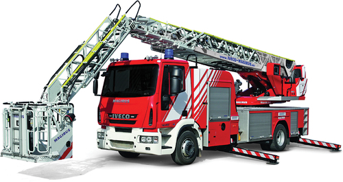
Turntable ladders are examples of mobile large-scale manipulators that are used by fire departments all over the world. As shown in Figure 1, the vehicle consists of a conventional truck chassis with additional support structure and telescopic extractable ladder parts mounted on a rotating frame. Turntable ladders are used to reach high positions (e.g. windows in a high building) for rescuing people in danger or extinguishing fires.

Figure 1. Turntable ladder M32L-AT from Magirus GmbH.

Unlike other large-scale manipulators, such as mobile cranes or elevating working platforms, turntable ladders need to consist of U-shaped segments providing an ascendable path inside the ladder parts. In combination with inevitable lightweight construction due to legal weight limitations (see (DIN EN 14043: 2014-04 2014)) and large ladder lengths up to 68 m, turntable ladders are susceptible to structural oscillations. Pertsch and Sawodny (2016) propose an active oscillation damping for turntable ladders that proves to be an effective way to increase speed, comfort and precision for operating turntable ladders. Multiple sensors are used to reconstruct the states of oscillations by an observer and a state controller is used to increase virtual damping for reducing the oscillations.

However, the model-based approach requires a high effort of conducting measurements to obtain precise identification data. Aiming to reduce the effort and cost of the control design process, a precise flexible multibody system representing all ladder parts is derived in (Densborn and Sawodny 2021) and later extended in (Densborn 2022). This dynamic model does not include the chassis and support structure of the vehicle, but it was shown that their stiffness influences the dynamic behaviour of the ladder oscillations significantly. Therefore, a dynamic model for the chassis including the outriggers and tires is derived in this paper to extend the previous model for obtaining an overall dynamic system of the entire vehicle. The resulting model aims for a simulation-based parametrization of the active damping control. Additionally, the support structure model can be used to analyse the outrigger contact forces in dynamic scenarios. These contact forces are crucial for mobile manipulators because the outreach limit calculations are one of the most important safety precautions. Potential approaches to determine dynamic outreach limits considering the tip-over stability can be examined with the presented dynamic model.

There is related research in the field of large-scale manipulators focusing on the support structure of mobile cranes or concrete pumps. Posiadala (1997) presents a dynamic model for a mobile crane that combines the dynamics of the flexible support structure with the pendulum motion. Similar models for mobile cranes are derived in (Trabka 2016) analysing the influence of the support structure onto the load trajectory and in (Jarzebowska et al. 2019) focusing on the vibration behaviour of the pendulum. A model for the support structure of concrete pumps is presented in (Kemmetmüller et al. 2021) aiming for optimizing its configuration. Wanner (2024) uses the support configuration of a concrete pump to define position limits for the manipulator during an automated movement. All these systems share a widely used vertical-horizontal support structure. In contrast, the turntable ladder in Figure 1 uses an uncommon V-shaped support structure which also does not lift the tires off the ground completely. Due to all differences, a newly derived dynamic model for the specific turntable ladder support structure is needed.

The dynamic model includes all outrigger forces which is interesting because the special support structure allows for one outrigger to become fully unloaded. Hasan et al. (2010) shows that knowledge about the outrigger forces helps in the planning and design of the system. Also Romanello (2018), and Romanello (2022) focus on outrigger forces to examine the tip-over stability for mobile cranes which is crucial for safety standards and very useful to determine essential outreach limits. However, most previous works perform static calculations without considering dynamics. In contrast, this paper provides a dynamic model that allows for analysis of contact forces and tip-over stability for dynamic trajectories.

In summary, the contributions of this paper are the following:

• Dynamic model of the chassis including flexible deformation and specific support structure system including the possibility of a fully unloaded outrigger.

• Parameter identification approach based on a sensitivity analysis and the Fisher-Information matrix.

• Validation of the resulting chassis model with quasi-static measurements.

• Validation with dynamic measurements after adding an existing flexible multibody system model for the ladder parts’ dynamics to get an overall dynamic system.

The remainder of this paper is structured as follows: Sec. 2 presents the derivation of the dynamic model. A suitable parameter identification approach based on a sensitivity analysis is described in Sec. 3. In Sec. 4, an outrigger lift-off prediction using the dynamical model is compared to measurements. Subsequently, the dynamic model is validated by measurements with dynamical excitation in Sec. 5 followed by a final conclusion in Sec. 6.

2. Derivation of the dynamic model

This section covers the derivation of a dynamic model for the undercarriage of the turntable ladder including the support structure. For this purpose, a multibody system with rigid bodies coupled by spring-damper elements is assumed and the dynamic equations are derived by using the Lagrange formalism. Details including the used parameters, degrees of freedom and kinematics are described in the following.

2.1. System description

To allow for deformations of the structure, the chassis is split into four parts leading to a multibody system which is depicted in Figure 2. Each rigid body $B_i$ with $\mathit{i}\in \{1,2,3,4\}$ is defined by its geometric dimensions, mass, and inertia given by known CAD (computer aided design) data. $B_1$ to $B_3$ are at the rear part of the vehicle located between the rear outriggers and the front outriggers. As the outmost rigid body $B_4$ at the front represents the driver’s cabin, its dimensions are significantly larger compared to the other bodies.

Figure 2. Mechanical structure of the entire multibody system (side view).

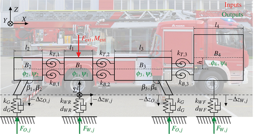
The inertial coordinate system ${\mathrm{\Sigma }}^I$ is located right below the swing bearing at ground level and the orientation is defined according to (DIN ISO 8855:2013-11 2013): The inertial $\mathit{x}$-axis is pointing to the front, parallel to the longitudinal axis of the vehicle and the $\mathit{z}$-axis points upwards in vertical direction to align with the rotational axis of the swing bearing.

According to the position and acceleration of the ladder, an external force ${\mathit{F}}_{\mathrm{ext}}$ and moment ${\mathit{M}}_{\mathrm{ext}}$ is induced at the swing bearing that excites the dynamic behaviour of the undercarriage. Therefore, these values combined represent the input for the dynamic system. As the first body $B_1$ is located directly underneath the swing bearing, the external force ${\mathit{F}}_{\mathrm{ext}}$ and moment ${\mathit{M}}_{\mathrm{ext}}$ are applied to it. All four parts $B_1$ to $B_4$ are aligned with the $\mathit{x}$-axis and they are connected by two-dimensional rotational joints. So, the bodies have two degrees of freedom each to enable a twisting and bending deformation of the chassis. These bodies can separately rotate around the $\mathit{x}$-axis with a displacement ${\varphi }_i$ (twisting) and also change their orientation around the $\mathit{y}$-axis by ${\psi }_i$ (bending). For allowing these deformations and transmitting the energy along the construction, there are three torsional stiffnesses ${\mathit{k}}_T={\left[{\mathit{k}}_{\mathit{T},1},k_{\mathit{T},2},k_{\mathit{T},3}\right]}^{\mathrm{\top }}$ and three bending stiffnesses ${\mathit{k}}_B={\left[{\mathit{k}}_{\mathit{B},1},k_{\mathit{B},2},k_{\mathit{B},3}\right]}^{\mathrm{\top }}$ modelled between two adjacent bodies. A rotational deformation around the $\mathit{z}$-axis is not needed for the model because the external forces and momentum are mainly induced by gravitation. The deformation angles are outputs of the dynamic system completed by all vertically acting ground contact forces of the outriggers $F_{\mathit{O},\mathit{j}}$ and wheels $F_{\mathit{W},\mathit{j}}$. Here, the index $\mathit{j}$ indicates one of the position rear right (RR), rear left (RL), front right (FR) and front left (FL), respectively. These contact forces are computed with the spring deformations $\mathrm{\Delta }{z}_{\mathit{O},\mathit{j}}$ and $\mathrm{\Delta }{z}_{\mathit{W},\mathit{j}}$ that are obtained by kinematic calculations.

Every body is connected by either tires or the outriggers leading to a contact point to the ground. Note that in contrast to many other mobile cranes with support structure, the turntable ladder’s tires always remain in contact to the ground even though the main load is absorbed by the outriggers. The tires are located beneath the two bodies $B_1$ and $B_4$ and are represented by spring-damper elements in the model that are added at the left and right side of the vehicle at different positions along the $\mathit{y}$-axis. As the rear axle is constructed more sturdy, two different parameters are used for the stiffnesses $k_{\mathit{WR}}$ and $k_{\mathit{WF}}$ representing the rear axle and front axle, respectively. The damping coefficients $d_{\mathit{WR}}$ and $d_{\mathit{WF}}$ are named accordingly.

The outriggers holding the main load of the ladder are mounted to the other two bodies $B_2$ and $B_3$ and their setup is shown more precise in Figure 3 from a rear view. Because of the characteristic placement of the outriggers, it is also called a V-shaped support structure.

Figure 3. Mechanical structure of the rear outriggers (rear view).

The upper cuboidal body is the rigid body $B_2$ representing the rear part of the chassis. The outriggers are mounted to the chassis and connected by rotational joints. The enclosed tilt angle is and ${\beta }_m={\beta }_0+\mathrm{\Delta }{\beta }_m$ with $\mathit{m}\in \{1,2,3,4\}$ where ${\beta }_0$ is the initial angle obtained from CAD data without considering any load. The relative displacements $\mathrm{\Delta }{\beta }_m$ are defined as degrees of freedom for the system. A rotational spring-damper element with stiffness $k_L$ and damping $d_L$ is placed in the corner of that link to represent the stiffness of that connection. At the end of each supporting leg, the outriggers are in contact to the ground. These contact points are represented in the model by a vertical spring-damper element with the parameters $k_G$ and $d_G$ modelling the resistance of the ground. Even though the contact points also have a displacement in $\mathit{y}$-direction due to the kinematics, this value is so minor that it is neglected. As the main load is the gravitational force of the ladder parts on top of the chassis, it is sufficient that the spring-damper element with $k_G$ and $d_G$ acts only in vertical direction.

Combining everything of the previously explained structure, the multibody system can be fully described with 13 degrees of freedom as

(1) $\mathit{q}={\left[\begin{array}{cccc}\mathbf{\Delta }{\mathit{\beta }}^{\mathrm{\top }}& {\mathit{\varphi }}^{\mathbf{\top }}& {\mathit{\psi }}^{\mathbf{\top }}& z_1\end{array}\right]}^{\mathrm{\top }}$(1)

where $\mathbf{\Delta }\mathit{\beta }$ are the relative tilt angles between the chassis and each supporting leg, $\mathit{\varphi }$ represents the twisting deformations and $\mathit{\psi }$ represents the bending deformation of all four bodies. The value $z_1$ describes the height of body $B_1$ and changes according to the load ${\mathit{F}}_{\mathrm{ext}}$. Its reference value for ${\mathit{F}}_{\mathrm{ext}}=\mathbf{0}$ and no deformations is chosen such that the contact points of the outriggers are exactly at ground level with $\mathrm{\Delta }{z}_{\mathit{O},\mathit{j}}=0$. All heights of the other bodies are not included in $\mathit{q}$, as they are calculated based on $z_1$ and the kinematic structure. The previously introduced stiffness and damping parameters are combined to

(2) $\mathit{k}={\left[\begin{array}{cccccc}{k}_L& k_G& {\mathit{k}}_T^{\mathrm{\top }}& {\mathit{k}}_B^{\mathrm{\top }}& k_{\mathit{WR}}& k_{\mathit{WF}}\end{array}\right]}^{\mathrm{\top }}$(2)

(3) $\mathrm{and}\mathit{d}={\left[\begin{array}{cccc}{d}_L& d_G& d_{\mathit{WR}}& d_{\mathit{WF}}\end{array}\right]}^{\mathrm{\top }}.$(3)

2.2. Kinematics

Each body of the multibody system has its own coordinate system defined by the kinematics of the system. For deriving the rotation matrix from each body $B_i$ with respect to the inertial frame the rotation matrices

(4) ${\mathit{R}}_x(\mathit{\gamma })=\left[\begin{array}{ccc}1& 0& 0\\ 0& cos(\mathit{\gamma })& -sin(\mathit{\gamma })\\ 0& sin(\mathit{\gamma })& cos(\mathit{\gamma })\end{array}\right],$(4)

(5) ${\mathit{R}}_y(\mathit{\gamma })=\left[\begin{array}{ccc}cos(\mathit{\gamma })& 0& sin(\mathit{\gamma })\\ 0& 1& 0\\ -sin(\mathit{\gamma })& 0& cos(\mathit{\gamma })\end{array}\right]$(5)

are used. As the deformation angles of the chassis are small with ${\varphi }_i,{\psi }_i<1^{\circ }$, the small-angles approximations $sin(\mathit{\gamma })\approx \mathit{\gamma }$ and $cos(\mathit{\gamma })\approx 1$ are applied to obtain ${\mathit{R}}_{\mathrm{x},\mathrm{lin}}$ and ${\mathit{R}}_{\mathrm{y},\mathrm{lin}}$. The resulting rotation matrix of body $B_i$ is then defined by

(6) ${\mathit{R}}_{IB}^i={\mathit{R}}_{\mathrm{y},\mathrm{lin}}({\psi }_i)\cdot {\mathit{R}}_{\mathrm{x},\mathrm{lin}}({\varphi }_i).$(6)

Additionally, the displacement vector of each coordinate system’s origin is needed for the kinematics. The position of the first body ${\mathit{r}}_{IB}^1$ is defined by solely the height $z_1$ and this body is the base of the kinematic tree. The constant $\mathit{x}$-coordinates of each body are calculated with the given lengths $l_i$. All $\mathit{y}$-coordinates are set to 0 constraining the bodies to be aligned along the longitudinal axis of the chassis. Therefore, the model does not allow a translation of the truck chassis in the $\mathit{xy}$-plane. This is based on the assumption that all displacements in the horizontal directions are negligibly small and not relevant for the given load ${\mathit{F}}_{\mathrm{ext}}$ and ${\mathit{M}}_{\mathrm{ext}}$ induced by gravitation. The $\mathit{z}$-coordinate of the bodies $B_2$, $B_3$ and $B_4$ are depending on $z_1$ and the bending deformations ${\psi }_i$. They are calculated by using the lengths $l_i$ and an additional height $\mathit{h}$ needed for $B_4$ as shown in Figure 2. Note that ${\psi }_i$ is the absolute value of the angle around the $\mathit{y}$-axis for body $B_i$ with respect to the inertial coordinate system. This leads to the displacement vectors

${\mathit{r}}_{IB}^1={\left[\begin{array}{ccc}0& 0& z_1\end{array}\right]}^{\mathrm{\top }}$

(7) ${\mathit{r}}_{IB}^2={\left[\begin{array}{ccc}-\frac{l_1}{2}-\frac{l_2}{2}& 0& z_1+\frac{l_1}{2}sin({\psi }_1)+\frac{l_2}{2}sin({\psi }_2)\end{array}\right]}^{\mathrm{\top }}$(7)

${\mathit{r}}_{IB}^3={\left[\begin{array}{ccc}\frac{l_1}{2}+\frac{l_3}{2}& 0& z_1-\frac{l_1}{2}sin({\psi }_1)-\frac{l_3}{2}sin({\psi }_3)\end{array}\right]}^{\mathrm{\top }}$

${\mathit{r}}_{IB}^4={\left[\begin{array}{ccc}\frac{l_1}{2}+l_3+\frac{l_4}{2}& 0& z_1+\mathit{h}-\frac{l_1}{2}sin({\psi }_1)-l_{3}sin({\psi }_3)-\frac{l_4}{2}sin({\psi }_4)\end{array}\right]}^{\mathrm{\top }}.$

Combining the orientation and the translational displacement of each coordinate system, the homogeneous transformation

(8) $T_{IB}^i=\left[\begin{array}{cc}{\mathit{R}}_{IB}^i& {\mathit{r}}_{IB}^i\\ \mathbf{0}& 1\end{array}\right]$(8)

is obtained. Similarly, the coordinate systems for the outriggers are derived considering the position of the connected body and additionally the twisting deformations ${\varphi }_i$ and the tilt angle ${\beta }_m$ of each outrigger. So, the outrigger contact points to the ground are the end points of the kinematic tree structure and the spring-damper displacements $\mathrm{\Delta }{z}_{\mathit{O},\mathit{j}}$ are depending on all degrees of freedom $\mathit{q}$. These displacements are then used to compute the contact forces described in Sec. 2.4.

Note that both outriggers (rear and front) are not at the exact same $\mathit{x}$-position along the longitudinal axis which is also influencing the kinematics. Due to the small difference in $\mathit{x}$-direction, the multibody system is not symmetric anymore comparing the left and right side.

For implementation, the software framework CasADi from (Andersson et al. 2019) is used. The automatic differentiation provides an efficient calculation for the derivative of each rotation matrix ${\mathit{R}}_{\mathit{IB}}$. Using this result, the rotational velocity of each body ${\omega }_i$ can be extracted by applying from (Siciliano et al. 2008).

(9) ${\mathbf{\Omega }}_{\mathit{IB}}={\dot{\mathit{R}}}_{\mathit{IB}}^{\mathit{i}}{\mathit{R}}_{IB}^{i\mathrm{\top }}\in {\mathbb{R}}^{3\times 3}$(9)

(10) ${\mathit{\omega }}_{\mathit{i}}=\frac{1}{2}\left[\begin{array}{c}{\mathbf{\Omega }}_{\mathit{IB}}(3,2)-{\mathbf{\Omega }}_{\mathit{IB}}(2,3)\\ {\mathbf{\Omega }}_{\mathit{IB}}(1,3)-{\mathbf{\Omega }}_{\mathit{IB}}(3,1)\\ {\mathbf{\Omega }}_{\mathit{IB}}(2,1)-{\mathbf{\Omega }}_{\mathit{IB}}(1,2)\end{array}\right]$(10)

2.3. Lagrange formalism

For deriving the dynamic equations, the Lagrange formalism is applied. The Lagrangian function

(11) $\mathcal{L}=\mathit{T}-\mathit{V}$(11)

is defined where $\mathit{T}$ is the total kinetic energy and $\mathit{V}$ the total potential energy of the overall system. The dynamic equations of motion are obtained by applying

(12) $\frac{\mathrm{d}}{\mathrm{d}t}{\left(\frac{\mathrm{\partial }\mathcal{L}}{\mathrm{\partial }\dot{\mathit{q}}}\right)}^{\mathrm{\top }}-{\left(\frac{\mathrm{\partial }\mathcal{L}}{\mathrm{\partial }\mathit{q}}\right)}^{\mathrm{\top }}=\mathit{\tau }$(12)

leading to a system of the form

(13) $\mathit{M}\left(\mathit{q}\right)\ddot{\mathit{q}}+\mathit{C}(\mathit{q},\dot{\mathit{q}},\mathit{u})=\mathit{\tau }\left(\mathit{u}\right).$(13)

The nonconservative forces $\mathit{\tau }$ depend on all damper forces and the input $\mathit{u}$ that combines the external forces ${\mathit{F}}_{\mathrm{ext}}$ and external moment ${\mathit{M}}_{\mathrm{ext}}$:

(14) $\mathit{\tau }\left(\mathit{u}\right)={\mathit{J}}_F^{\mathrm{\top }}{\mathit{F}}_{\mathrm{ext}}+{\mathit{J}}_M^{\mathrm{\top }}{\mathit{M}}_{\mathrm{ext}}-\sum _{\mathit{\mu }=1}^{{\mathit{n}}_{\mathit{CP}}}{\mathit{J}}_{\mu }^{\mathrm{\top }}{d}_{\mu }\mathrm{\Delta }{\dot{\mathit{z}}}_{\mathit{\mu }}-\sum _{\mathit{m}=1}^4{\mathit{J}}_m^{\mathrm{\top }}{d}_L\mathrm{\Delta }{\dot{\beta }}_{\mathit{m}}.$(14)

The Jacobians ${\mathit{J}}_F=\frac{{\mathrm{\partial }}_I{\mathit{r}}_{{\mathit{F}}_{\mathrm{ext}}}}{\mathrm{\partial }\mathit{q}}$, ${\mathit{J}}_M=\frac{{\mathrm{\partial }}_I{\mathit{\omega }}_1}{\mathrm{\partial }\dot{\mathit{q}}}$, ${\mathit{J}}_{\mu }=\frac{{\mathrm{\partial }}_I{\mathit{r}}_{\mu }}{\mathrm{\partial }\mathit{q}}$ or ${\mathit{J}}_m=\frac{\mathrm{\partial }\mathrm{\Delta }{\dot{\beta }}_{\mathit{m}}}{\mathrm{\partial }\dot{\mathit{q}}}$ correspond to the degree of freedom where the respective force or moment is acting and transform all forces to the generalized coordinates frame. Here, $n_{\mathit{CP}}=8$ depicts the number of contact points to the ground in the system with $\mathrm{\Delta }{\mathit{z}}_{\mu }$ being the displacement of the respective damper element with damping coefficient $d_{\mu }$, namely $d_G$, $d_{\mathit{WR}}$ or $d_{\mathit{WF}}$. The overall kinetic energy of the system is given by

(15) $\mathit{T}=\sum _{\mathit{i}=1}^{n_B}\left(\frac{1}{2}{m}_i{\mathit{v}}_i^{\mathrm{\top }}{\mathit{v}}_i+\frac{1}{2}{\mathit{\omega }}_i^{\mathrm{\top }}{\mathit{I}}_i{\mathit{\omega }}_i\right)$(15)

where $n_B=8$ is the amount of bodies in the system including four bodies for the vehicle chassis $B_1$ to $B_4$ and four bodies for the outriggers. The velocities ${\mathit{v}}_i$ and ${\omega }_i$ of each body are computed in the inertial frame and the values of the masses $m_i$ and inertias ${\mathit{I}}_i$ are taken from CAD data. The overall potential energy is computed by

(16) $\mathit{V}=\sum _{\mathit{i}=1}^{n_B}\left(m_i{\mathit{g}}^{\mathrm{\top }}{\mathit{r}}_{IB}^i\right)+\sum _{\mathit{\mu }=1}^{{\mathit{n}}_{\mathit{CP}}}\frac{1}{2}{k}_{\mu }\cdot \mathrm{\Delta }{z}_{\mu }^2+\sum _{\mathit{m}=1}^4\frac{1}{2}{k}_L\cdot \mathrm{\Delta }{\beta }_m^2$(16)

(17) $\dots +\sum _{\hat{i}=1}^3\frac{1}{2}{k}_{T,\hat{i}}\cdot \mathrm{\Delta }{\varphi }_{\hat{i}}^2+\sum _{\hat{i}=1}^3\frac{1}{2}{k}_{B,\hat{i}}\cdot \mathrm{\Delta }{\psi }_{\hat{i}}^2$(17)

where $\mathit{g}={\left[\begin{array}{ccc}0& 0& 9.81\end{array}\right]}^{\mathrm{\top }}$ is the gravitational acceleration needed to compute the potential energy of each body. Index $\mathit{\mu }$ again represents all contact points to the ground with stiffness constants $k_G$, $k_{\mathit{WR}}$ or $k_{\mathit{WF}}$. Also, $\mathrm{\Delta }{\varphi }_{\hat{i}}$ and $\mathrm{\Delta }{\psi }_{\hat{i}}$ indicate the difference of the twisting or bending angles of two adjacent bodies where the stiffness $k_{T,\hat{i}}$ and $k_{B,\hat{i}}$ is placed.

2.4. Outputs

The output $\mathit{y}={\left[\begin{array}{cccc}{\mathit{F}}_O^{\mathrm{\top }}& {\mathit{F}}_W^{\mathrm{\top }}& {\mathit{\varphi }}^{\mathbf{\top }}& {\mathit{\psi }}^{\mathbf{\top }}\end{array}\right]}^{\mathrm{\top }}$ of the system during the identification measurements is defined with the measurable quantities

(18a) ${\mathit{F}}_O={\left[\begin{array}{cccc}{\mathit{F}}_{\mathit{O},\mathit{RR}}& F_{\mathit{O},\mathit{RL}}& F_{\mathit{O},\mathit{FR}}& F_{\mathit{O},\mathit{FL}}\end{array}\right]}^{\mathrm{\top }}$(18a)

(18b) ${\mathit{F}}_W={\left[\begin{array}{cccc}{\mathit{F}}_{\mathit{W},\mathit{RR}}& F_{\mathit{W},\mathit{RL}}& F_{\mathit{W},\mathit{FR}}& F_{\mathit{W},\mathit{FL}}\end{array}\right]}^{\mathrm{\top }}$(18b)

(18c) $\mathit{\varphi }={\left[\begin{array}{cccc}{\varphi }_1& {\varphi }_2& {\varphi }_3& {\varphi }_4\end{array}\right]}^{\mathrm{\top }}$(18c)

(18d) $\mathit{\psi }={\left[\begin{array}{cccc}{\psi }_1& {\psi }_2& {\psi }_3& {\psi }_4\end{array}\right]}^{\mathrm{\top }}.$(18d)

In total, 16 outputs can be measured, where the first eight outputs are the contact forces on each connection point to the ground measured by special scales. The four contact forces of the outriggers are computed by

(19) $F_{\mathit{O},\mathit{j}}=k_G\mathrm{\Delta }{z}_{\mathit{O},\mathit{j}}+d_G\mathrm{\Delta }{\dot{z}}_{\mathit{O},\mathit{j}}.$(19)

The four wheel forces $F_{\mathit{W},\mathit{i}}$ are similarly computed with the parameters of the front and rear tires, respectively:

(20) $F_{\mathit{W},\mathit{j}}=k_{\mathit{WR}}\mathrm{\Delta }{z}_{\mathit{W},\mathit{j}}+d_{\mathit{WR}}\mathrm{\Delta }{\dot{z}}_{\mathit{W},\mathit{j}},\mathit{j}\in \{\mathit{RR},\mathit{RL}\}$(20)

(21) $F_{\mathit{W},\mathit{j}}=k_{\mathit{WF}}\mathrm{\Delta }{z}_{\mathit{W},\mathit{j}}+d_{\mathit{WF}}\mathrm{\Delta }{\dot{z}}_{\mathit{W},\mathit{j}},\mathit{j}\in \{\mathit{FR},\mathit{FL}\}.$(21)

The last outputs are the four twisting angles ${\varphi }_i$ of each body and the four bending angles ${\psi }_i$ representing the flexible deformation of the chassis. The absolute angles are measured with inclination sensors mounted to the mechanical structure.

2.5. Special case: a fully unloaded outrigger

For modelling the contact points of the outriggers and tires with spring-damper elements it is crucial that forces can only be transmitted when the contact persists. However, the turntable ladder is designed to allow that one of four outriggers is possibly fully unloaded when the outreach is close to its maximum. In this case, there is no force transmitted between the multibody system and the ground for the respective outrigger $\mathit{j}$ leading to $F_{\mathit{O},\mathit{j}}=0$ while all other three outriggers and all tires carry the entire load of the vehicle. Note that only outriggers can become fully unloaded while the contact forces of the tires remain all the time.

For including this case into the dynamic model, the stiffness representing the ground $k_G$ is adapted to enable a representation of a fully unloaded outrigger. This approach is motivated by the nonlinear approximation of the contact forces of a concrete pump support structure in Kemmetmüller et al. (2021). Whenever the outrigger is fully unloaded, the displacement of the respective spring-damper element is positive. So, for $\mathrm{\Delta }{z}_{\mathit{O},\mathit{j}}\ge 0$ the stiffness and damping is set to zero $k_{\mathit{G},\mathit{j}}=0$. The resulting nonlinear stiffness $k_{\mathit{G},\mathit{nl}}$ is illustrated in Figure 4.

Figure 4. Nonlinear stiffness model for a fully unloaded outrigger.

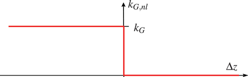
The nonlinear stiffness is expressed by the equation

(22) $k_{\mathit{G},\mathit{nl}}=\left\{\begin{array}{cc}{k}_G& ,\mathrm{\Delta z}<0\\ 0& ,\mathrm{\Delta z}\ge 0.\end{array}\right.$(22)

The possibility to avoid the discontinuity was examined by introducing a small transition region with a linear decrease from $k_G$ to $0$. However, no significant improvement was noted. Therefore, the nonlinear stiffness from (22) is used. The same procedure is applied for the damping coefficient $d_G$.

3. Parameter identification

A parameter identification is needed to find numerical values of each parameter that is used in the model from Sec. 2.

3.1. Measurement for parameter identification

Identification measurements are conducted using a turntable ladder from the manufacturer Magirus. Note that the sensor outputs defined in (18a) to (18d) are specifically for identification purposes and not included in the serial product. The contact forces in (18a) and (18b) are measured with special wheel load scales with a resolution of 10 kg and a sampling time of 1.2 s. The inclination sensors for measuring the deformation angles in (18c) and (18d) have a resolution of ${0.04}^{\circ }$ and a sampling time of 20 ms.

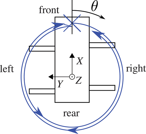
The applied process is as follows: The ladder is extracted close to the maximum ladder length for a constant elevation angle to induce a large excitation of the chassis deformation resulting in large differences of the contact forces. The ladder is controlled to perform a rotation with a low and constant velocity starting at the swing angle $\mathit{\theta }=0$ and ending at $\mathit{\theta }=2\mathit{\pi }$. After that, the ladder is also moved in the opposite direction to the starting point $\mathit{\theta }=0$ in the same measurement to avoid any dependency on the rotation direction. This movement is sketched in Figure 5 by an aerial view on the vehicle.

Figure 5. Path of the ladder movement during the measurements.

Due to the low velocity with $\dot{\theta }\approx 2^{\circ }/\mathit{s}$, the measurement can be stated as quasi-static. Therefore, only the gravitational force of the ladder with mass $m_{\mathrm{ladder}}$ is considered leading to

(23) ${\mathit{F}}_{\mathrm{ext}}=\left[\begin{array}{c}{F}_x\\ F_y\\ F_z\end{array}\right]=\left[\begin{array}{c}0\\ 0\\ -9.81\mathrm{m}/{\mathrm{s}}^2\cdot m_{\mathrm{ladder}}\end{array}\right]$(23)

and the external moment

(24) ${\mathit{M}}_{\mathrm{ext}}=\left[\begin{array}{c}{M}_x\\ M_y\\ M_z\end{array}\right]=\left[\begin{array}{c}\parallel M_{\mathrm{abs}}\parallel \cdot sin(\mathit{\theta })\\ \parallel M_{\mathrm{abs}}\parallel \cdot cos(\mathit{\theta })\\ 0\end{array}\right]$(24)

where $\parallel M_{\mathrm{abs}}\parallel$ is the amplitude of the resulting moment depending on the chosen ladder length. The values of ${\mathit{F}}_{\mathrm{ext}}$ and ${\mathit{M}}_{\mathrm{ext}}$ cannot be directly measured, but they can be precisely calculated with given ladder length $\mathit{L}$ and its elevation angle $\mathit{\alpha }$. The measured strain gauges at the ladder parts proof that there are no noteworthy structural oscillations during this measurement that falsify the quasi-static measurements.

After conducting the measurements, all outputs are approximated by periodic functions to remove any effects that do not respect the dynamic model, e.g. measurement offsets. The deformation of the vehicle chassis can be approximated by

(25) $\begin{array}{cc}{\varphi }_i& =A_{\mathit{\varphi },\mathit{i}}\cdot sin(\mathit{\theta })+{\varphi }_{\mathrm{off},i}\\ {\psi }_i& =A_{\mathit{\psi },\mathit{i}}\cdot cos(\mathit{\theta })+{\psi }_{\mathrm{off},i}.\end{array}$(25)

The parameter identification then aims to fit the amplitudes $A_{\mathit{\varphi },\mathit{i}}$ and $A_{\mathit{\psi },\mathit{i}}$. However, the measured offsets ${\varphi }_{\mathrm{off},i}$ and ${\psi }_{\mathrm{off},i}$ are neglected for the parameter identification. The offsets occur due to non ideal evenness of the ground and cannot be represented by the model that assumes an even ground.

The measured contact forces can be approximated by

(26) $F_{0,\mathit{j}}=max\left(F_{\mathit{O},\min },A_{\mathit{O},\mathit{j}}\cdot sin(\mathit{\theta }+{\theta }_0)+F_{\mathit{O},\mathrm{off},j}\right)$(26)

(27) $F_{\mathit{W},\mathit{j}}=A_{\mathit{W},\mathit{j}}\cdot sin(\mathit{\theta }+{\theta }_0)+F_{\mathit{W},\mathrm{off},j}.$(27)

For approximating the outrigger forces, a special case needs to be considered because of its construction, see Figure 6. Even when the outrigger is fully unloaded and there is no force transmitted between the outrigger beam and outrigger plate, the outrigger plate will not lift off the ground at any time in reality. This is a mandatory safety feature for those kind of vehicles defined by (DIN EN 14043: 2014-04 2014). So, the measured outrigger force will always include the gravitational force of the outrigger plate that provides a lower bound of the measured forces of $F_{\mathit{O},\min }\approx 500\mathrm{N}$. As the tires will never become fully unloaded, the special case is not considered here and it can be described by a conventional sinusoidal wave. The previously described approximations of each output are used for fitting the parameters in the identification process.

Figure 6. Construction of the outrigger contact to the ground.

3.2. General setup of parameter identification

The aim is to identify an optimal parameter set ${\mathit{p}}^{\ast }$ such that the simulated output ${\mathit{y}}_s$ represent the measured output ${\mathit{y}}_m$ as close as possible. This identification can be formulated as an optimization problem with

(28) ${\mathit{p}}^{\ast }=arg\underset{\mathit{p}\in P}{min}\mathit{J}$(28)

where $\mathit{P}$ is a set of all physically possible parameters and $\mathit{J}$ is a cost function to be minimized. It is defined as the squared absolute error between measured and simulated output:

(29) $\mathit{J}=\sum _{\mathit{n}=1}^N\sum _{\mathit{i}=1}^{16}{w}_i\cdot s_i\cdot (y_{\mathit{m},\mathit{i}}[\mathit{n}]-y_{\mathit{s},\mathit{i}}[\mathit{n}]{)}^2.$(29)

$w_i$ are respective weighting factors that are initially set to $1$. Whenever the value of $w_i$ is changed, it is mentioned in Sec. 3.4. The values $s_i$ are additional scaling factors for each output. These scaling factors $s_i$ are needed because the magnitude of each outputs are significantly different and the error of each output should have an equal influence to the cost function $\mathit{J}$ and they are set to the value

(30) $s_i=\frac{1}{{\left(max({\mathit{y}}_{\mathit{m},\mathit{i}})-min(y_{\mathit{m},\mathit{i}})\right)}^2}.$(30)

Additionally, the weighting factors $w_i$ are used to favour a fit to specific outputs. For example, when the goal is to examine the unloaded outriggers, the weighting factors $w_i$ of the outrigger forces are chosen relatively larger compared to the other weighting factors. The measurement interval $\mathit{\theta }\in \left[{0,360}^{\circ }\right]$ is sampled at $5^{\circ }$ steps leading to $\mathit{N}=73$ points. The cost function $\mathit{J}$ sums over the fit for each sample point of $\mathit{\theta }$.

As the system input $\mathit{u}$ from Section 3.1 only includes low velocities and is quasi-static, the exact values of the damping coefficients $\mathit{d}$ do not have significant impact on the simulated output ${\mathit{y}}_s$. However, numerical problems occur when setting the damping coefficients to $\mathit{d}=\mathbf{0}$ resulting in high frequency oscillations in simulation that are not related to the system dynamics. To avoid these numerical problems, the damping coefficients are set to nonzero values. For the sake of simplicity, all values in $\mathit{d}$ are chosen equally. The values were increased iteratively to determine a suitable value for $\mathit{d}$ empirically. After this procedure, the damping coefficient are set to

(31) $d_L=1\cdot {10}^4\mathrm{Nms}/\mathrm{rad},d_G=d_{\mathit{WR}}=d_{\mathit{WF}}=1\cdot {10}^4\mathrm{Ns}/\mathrm{m}.$(31)

Thus, it is inferred that the parameter vector $\mathit{p}$ for the optimization in the identification process should only contain the stiffnesses $\mathit{k}$. Note that the damping coefficients from (34) not only achieve good results for a quasi-static input, but they are also set to the same values for the dynamic simulation in Sec. 5.

3.3. Identifiability and sensitivity analysis

The identifiability of the parameter vector $\mathit{p}=\mathit{k}$ with the given measurable output $\mathit{y}$ is shown. The equations of motion in (13) and the output equations in (18a) to (18d) are used to obtain the general nonlinear system

(32) $\dot{\mathit{x}}=\mathit{f}\left(\mathit{x},\mathit{u},\mathit{p}\right)$(32)

(33) $\mathit{y}=\mathit{h}(\mathit{x},\mathit{u},\mathit{p})$(33)

by defining the states $\mathit{x}={\left[\begin{array}{cc}{\mathit{q}}^{\mathrm{\top }}& {\dot{\mathit{q}}}^{\mathrm{\top }}\end{array}\right]}^{\mathrm{\top }}$. Note that the dimensions of the system are $\mathit{p}=\mathit{k}\in {\mathit{R}}^{10},\mathit{q}\in {\mathit{R}}^{13},\mathit{x}\in {\mathit{R}}^{26},\mathit{y}\in {\mathit{R}}^{16}$. For showing the identifiability of the parameter vector $\mathit{p}$, a nonlinear observability analysis – see (Horacio 2003) – is applied to the extended state vector

(34) $\bar{\mathit{x}}=\left[\begin{array}{c}\mathit{x}\\ \mathit{p}\end{array}\right].$(34)

An output mapping $\mathrm{\Gamma }$ is defined that includes the output $\mathit{y}$ and its derivative yielding

(35) $\mathrm{\Gamma }={\left[\begin{array}{cc}{\mathit{y}}^{\mathrm{\top }}& {\dot{\mathit{y}}}^{\mathrm{\top }}\end{array}\right]}^{\mathrm{\top }}$(35)

and the local observability matrix ${\mathit{Q}}_{\mathrm{obs}}$ is computed by

(36) ${\mathit{Q}}_{\mathrm{obs}}={\left(\frac{\mathrm{\partial }\mathrm{\Gamma }}{\mathrm{\partial }\bar{\mathit{x}}}{|}_{\mathit{x},\mathit{p},\mathit{u}}\right)}^{\mathrm{\top }}\left(\frac{\mathrm{\partial }\mathrm{\Gamma }}{\mathrm{\partial }\bar{\mathit{x}}}{|}_{\mathit{x},\mathit{p},\mathit{u}}\right)\in \mathbb{R}{ }^{n_{\bar{x}}\times n_{\bar{x}}}.$(36)

For showing the identifiability of parameters $\mathit{p}$, only the partial matrix ${\mathit{Q}}_{\mathrm{part}}\in {\mathit{R}}^{n_p\times n_p}$ is of interest which is the last $n_p$ rows and columns of ${\mathit{Q}}_{\mathrm{obs}}$. It is confirmed that the matrix ${\mathit{Q}}_{\mathrm{part}}$ has full rank and therefore, all parameters in the vector $\mathit{p}$ are identifiable with the used input.

Additionally, a parameter sensitivity analysis based on (Müller et al. 2022) is applied to the dynamic multibody system to obtain more relevant information for the identification. Here, the approach is extended by suitable scaling factors. As described in (Skogestad and Postlethwaite 2005), a MIMO-system needs to be scaled with respect to its inputs and outputs. When comparing the output sensitivities ${\mathit{S}}_y=\frac{\mathrm{\partial }\mathit{y}}{\mathrm{\partial }\mathit{p}}\in {\mathit{R}}^{n_y\times n_p}$, the nominal values of $\mathit{p}$ should not influence the result. Therefore, a scaling with respect to the parameter vector $\mathit{p}$ is crucial to allow for a meaningful interpretation of the sensitivity analysis. Instead of using $\mathit{p}=\mathit{k}$, solely for the purpose of the sensitivity analysis, a new vector $\hat{\mathit{p}}$ is defined. It has the same length as $\mathit{p}$, but all entries are equal to $1$. Subsequently, the model is derived with the stiffness vector

(37) $\hat{\mathit{k}}={\mathit{k}}_{\mathit{SA}}\circ \hat{\mathit{p}}$(37)

where $\circ$ is the element-wise multiplication. ${\mathit{k}}_{\mathit{SA}}$ represents the nominal values of the stiffnesses during the sensitivity analysis. As the parameters are not yet identified, these values are obtained by a global optimization such that the simulated output is roughly in the range of the measurements. Applying this scaling procedure, all partial derivatives with respect to $\hat{p}$ needed for the sensitivity analysis can be derived. Also, all entries in $\hat{p}$ have the same value, such that the influence of each parameter value itself is equalized by the scaling.

The sensitivities of states ${\mathit{S}}_x=\frac{\mathrm{\partial }\mathit{x}}{\mathrm{\partial }\hat{\mathit{p}}}$ and the output sensitivities ${\mathit{S}}_y=\frac{\mathrm{\partial }\mathit{y}}{\mathrm{\partial }\hat{\mathit{p}}}$ describe how one single parameter influences the respective state or output. These sensitivities can be computed with the sensitivity differential equations (SDE) given by

(38 ${\dot{\mathit{S}}}_{\mathit{x}}=\frac{\mathrm{\partial }\mathit{f}}{\mathrm{\partial }\mathit{x}}{\mathit{S}}_x+\frac{\mathrm{\partial }\mathit{f}}{\mathrm{\partial }\hat{\mathit{p}}},\mathit{t}>0,{\mathit{S}}_x\left(0\right)=\frac{\mathrm{\partial }{\mathit{x}}_0}{\mathrm{\partial }\hat{\mathit{p}}}$(38

(39) ${\mathit{S}}_y=\frac{\mathrm{\partial }\mathit{h}}{\mathrm{\partial }\mathit{x}}{\mathit{S}}_x+\frac{\mathrm{\partial }\mathit{h}}{\mathrm{\partial }\hat{\mathit{p}}},\mathit{t}\ge 0$(39)

as presented in (Schmidt et al. 2010) or in (Bestle 1994). These SDE are solved simultaneously to the conventional ordinary differential equation of the system while simulating the dynamics. After simulating the SDE (41) and (42) to obtain the output sensitivity ${\mathit{S}}_{\mathit{y}}^{\mathrm{s}\mathrm{i}\mathrm{m}}$, this matrix is scaled with respect to the absolute value of the simulated outputs. This is necessary due to the different units resulting in significant different ranges of the outputs’ values. For this purpose, a scaling matrix

(40) $Y_{\mathit{sc}}=\mathrm{diag}\left(\frac{1}{{\mathit{y}}_{1,\max }},\frac{1}{{\mathit{y}}_{2,\max }},\dots ,\frac{1}{{\mathit{y}}_{16,\max }}\right)$(40)

is defined and the scaled output sensitivity matrix is obtained by

(41) ${\mathit{S}}_y^{\mathrm{s}\mathrm{c}\mathrm{aled}}=Y_{\mathit{sc}}\cdot {\mathit{S}}_y^{\mathrm{s}\mathrm{i}\mathrm{m}}.$(41)

Using the scaled output sensitivity matrix ${\mathit{S}}_{\mathit{y}}^{\mathrm{s}\mathrm{c}\mathrm{aled}}$, the Fisher-Information matrix (FIM) – see (Ljung 1999) – is derived by

(42) $\mathit{F}(\mathit{p},\mathit{u})=\sum \sum _{t_k=1}^{N_t}{\mathit{S}}_y^{\mathrm{s}\mathrm{c}\mathrm{aled}}[t_k{]}^{\mathrm{\top }}{\mathit{S}}_y^{\mathrm{s}\mathrm{c}\mathrm{aled}}[t_k]$(42)

where $t_k$ is a time step of the simulation. The FIM has full rank showing the identifiability of all parameters in $\mathit{p}$. However, some additional information can be extracted from the FIM when observing the eigenvalues $\mathit{\lambda }$ because small eigenvalues are related to larger variances which is obstructive for parameter identification. Sorting the eigenvalues of the FIM leads to

(43) ${\lambda }_1>{\lambda }_2>\dots >{\lambda }_8>{\lambda }_9\gg {\lambda }_{10}$(43)

(44) $1.92\cdot {10}^4>5.23\cdot {10}^3>\dots >203>80.5\gg 0.02$(44)

showing that the last eigenvalue is significantly lower compared to the others. The procedure described in (Majer 1998) and applied in (Müller et al. 2022) is used to find the related parameter. For that, the eigenvector matrix $\mathit{V}=[{\mathit{v}}_1,\dots ,{\mathit{v}}_{10}]$ is examined. The related parameter to ${\lambda }_{10}$ is indicated by the row in which the highest entry of the normed eigenvector ${\mathit{v}}_{10}$ is found. In this case, it is found in second row with value $max({\mathit{v}}_{10})=0.99$ which indicates a strong relation to the parameter $k_G$.

Appropriately, it is discovered that the highest three eigenvalues ${\lambda }_1$, ${\lambda }_2$ and ${\lambda }_3$ are related to the three parameters $k_L$, $k_{\mathit{WF}}$ and $k_{\mathit{WR}}$, respectively. Again, the highest entry in the respective eigenvector holds $max(\mathit{v})\ge 0.9$ which is showing a clear relation between the eigenvalue and the parameter. The remaining six eigenvalues are connected to the torsional and bending stiffnesses ${\mathit{k}}_T$ and ${\mathit{k}}_B$. This information is useful when designing the identification setup that is described in the following.

3.4. Identification approach

As already described, the identification process aims to find numerical values for the parameter vector including all stiffnesses

(45) $\mathit{k}={\left[\begin{array}{cccccc}{k}_L& k_G& {\mathit{k}}_T^{\mathrm{\top }}& {\mathit{k}}_B^{\mathrm{\top }}& k_{\mathit{WR}}& k_{\mathit{WF}}\end{array}\right]}^{\mathrm{\top }}.$(45)

Because of the significant differences in the output sensitivities of each parameter, it is beneficial not to optimize all parameters simultaneously. The sensitivity analysis in Sec. 3.3 shows the low sensitivity of $k_G$ which can be explained by two main reasons: First, the same $F_{\mathit{O},\mathit{j}}$ can be achieved with different spring deformations $\mathrm{\Delta }{z}_{\mathit{O},\mathit{j}}$ depending on the stiffness $k_G$. Second, the link stiffness $k_L$ effects the same outputs as parameter $k_G$. Therefore, it is proposed to set $k_G$ to a specific value and not include it in the identification process. Choosing $k_G=1\cdot {10}^8\mathrm{N}/\mathrm{m}$ leads to a limit of the spring deformation with $\mathrm{\Delta }{z}_{\mathit{O},\mathit{j}}<1\mathrm{mm}$ which is a desirable behaviour assuming the vehicle standing on a hard surface like concrete streets. For identifying all other parameters, it is proposed to split up the identification process into two different runs:

Run 1: The torsional stiffnesses ${\mathit{k}}_T$ and the bending stiffness ${\mathit{k}}_B$ are shown to have small sensitivities, too. Therefore, the values of these parameters are fixed for the first run to a specific value that is determined by finite element method (FEM) using the CAD data of the construction. For this calculation, suitable conditions are defined and a virtual moment is applied to the CAD model. The FEM simulation yields a displacement of the respective angle and the resulting stiffness is calculated. When using these FEM-based parameters for the first optimization run, only three remaining stiffnesses

(46) ${\mathit{p}}_{\mathrm{Run}1}={\left[\begin{array}{ccc}{k}_L& k_{\mathit{WR}}& k_{\mathit{WF}}\end{array}\right]}^{\mathrm{\top }}$(46)

are optimized. These stiffnesses in ${\mathit{p}}_{\mathrm{Run}1}$ have the largest sensitivities and are especially significant for determining the ground contact forces. As the focus of Run 1 is on the outrigger forces, the respective weighting factor in the cost function (32) is set to $w_{F_O}=3$ while all other weighting factors are $1$. For minimizing the cost function $\mathit{J}$ in Run 1 a genetic algorithm is chosen, because there is not much information about the range of the parameters and this algorithm only requires lower and upper bounds. The lower limit is set to zero to achieve nonnegative stiffnesses and the upper limit is set to a realistic value to avoid numerical problems in the simulation due to infinite stiffnesses.

Run 2: The result of the first optimization run ${\mathit{p}}_{\mathrm{R}\mathrm{u}\mathrm{n}1}^{\ast }$ is used as initial value for the second run that now uses a local optimization algorithm (Nelder-Mead Method, see e.g. (Nocedal and Wright 2006)). As the values for ${\mathit{k}}_T$ and ${\mathit{k}}_B$ from the finite element analysis (FEA) are not completely reliable, these parameters are optimized in Run 2. In contrary, only the two stiffnesses $k_L$ and $k_G$ are fixed to find a suitable parameter set with these values. This leads to the parameter set

(47) ${\mathit{p}}_{\mathrm{Run}2}={\left[\begin{array}{cccc}{\mathit{k}}_T^{\mathrm{\top }}& {\mathit{k}}_B^{\mathrm{\top }}& k_{\mathit{WR}}& k_{\mathit{WF}}\end{array}\right]}^{\mathrm{\top }}.$(47)

Since the torsional and bending stiffnesses have a high sensitivity onto the outputs ${\varphi }_i$ and ${\psi }_i$, the weighting factor of these outputs are increased in (32) to $w_{\varphi }=w_{\psi }=2$ aiming for a better fit of these angles. As the tire stiffnesses $k_{\mathit{WR}}$ and $k_{\mathit{WF}}$ also have a high sensitivity to the outputs ${\varphi }_i$, these parameters need to be included in the optimization in both runs. However, due to the local optimization in Run 2, the values are not changing significantly compared to the previously obtained values.

Summary of Both Identification Runs:

• Run 1:

Global optimization using genetic algorithm.

Parameters ${\mathit{k}}_T$ and ${\mathit{k}}_B$ are fixed and obtained by FEA.

Increase weightings $w_{F_O}$ in $\mathit{J}$ for the outrigger forces ${\mathit{F}}_O$.

• Run 2:

Previous result is starting value for local optimization.

Only $k_L$ and $k_G$ are fixed, other parameters are optimized.

Increase weightings $w_{\varphi }$ and $w_{\psi }$ for deformation angles.

With the previously described procedure of splitting the parameter identification in two consecutive optimization runs, a better result for the idenitified parameter set ${\mathit{p}}^{\ast }$ is achieved compared to optimizing all parameters at once.

3.5. Results of parameter identification

Applying the previous explained parameter identification approach yields the optimized parameters

${\mathit{p}}^{\ast }=[2.08\cdot {10}^7\mathrm{Nm}/\mathrm{rad},1.00\cdot {10}^8\mathrm{Nm},\dots$

$3.78\cdot {10}^7\mathrm{Nm}/\mathrm{rad},1.72\cdot {10}^7\mathrm{Nm}/\mathrm{rad},7.05\cdot {10}^5\mathrm{Nm}/\mathrm{rad},\dots$

$4.12\cdot {10}^7\mathrm{Nm}/\mathrm{rad},3.47\cdot {10}^7\mathrm{Nm}/\mathrm{rad},1.85\cdot {10}^6\mathrm{Nm}/\mathrm{rad},\dots$

$1.15\cdot {10}^6\mathrm{N}/\mathrm{m},4.44\cdot {10}^6\mathrm{Nm}/\mathrm{rad}{]}^{\mathrm{\top }}$

including all stiffnesses $\mathit{k}$ with dimension and order as stated in (45). This parameter set ${\mathit{p}}^{\ast }$ is used to simulate the dynamics and the results are compared to the measurements. The two states ${\varphi }_1$ and ${\psi }_1$ representing the deformation at the swing bearing (body $B_1$) are shown in Figure 7. Due to the quasi-static measurements, the following plots are depicted with dependency on the swing angle $\mathit{\theta }$ instead of the simulation time. Note that two different measurements were executed with different ladder lengths and elevation angles that both result in the same external load $M_{\mathrm{abs}}$. The measurement data was filtered with a low pass filter using a cutoff frequency $f_c=100\mathrm{Hz}$ to suppress measurement noise. It can be seen that the output follows the approximations in (25) and both measurements are nearly equivalent, as their amplitude only differs by $2\mathrm{\%}$ and $4\mathrm{\%}$ for ${\varphi }_1$ and ${\psi }_1$, respectively. The simulated outputs do not perfectly fit because the choice of the weighting factors $w_i$ in the cost function is in favor for fitting the outrigger forces. The mean absolute error is ${0.053}^{\circ }$ for ${\varphi }_1$ and ${0.071}^{\circ }$ for ${\psi }_1$, when the simulation is compared to the measured angles as they are used for the optimization in (29). With different design of the identification process, the fit of the angles ${\varphi }_1$ and ${\psi }_1$ could still be increased. However, the accuracy of the deformation angles ${\varphi }_1$ and ${\psi }_1$ are sufficient for focusing on the prediction of an fully unloaded outrigger as presented in Sec. 4. For this task, the fit of the simulated outrigger forces as shown in Figure 8 is more relevant.

Figure 7. Comparing two measurements of ${\varphi }_1$ and ${\psi }_1$ with the simulated output using optimized parameter ${\mathit{p}}^{\ast }$.

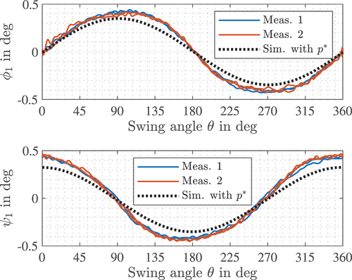
Figure 8. Comparing measurements of all outrigger forces $F_{\mathit{O},\mathit{j}}$ with the simulation using the optimized parameters ${\mathit{p}}^{\ast }$.

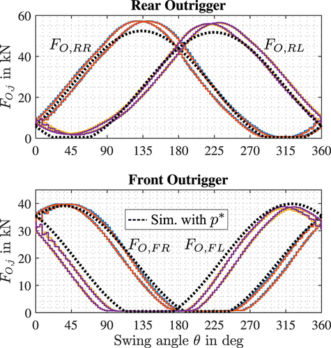
The measurements of the outrigger forces are shifted slightly comparing the different directions of the angular velocity due to the sampling time $T_s=1.2\mathit{s}$ of the wheel scales. Even though the velocity is not high, there is some dependency on the direction of the velocity. It can be observed that during the measurement three out of four outriggers are fully unloaded at some point. However, the forces are not completely symmetrical when comparing the left and right outriggers. This is mainly due to irreversible effects when operating the ladder and unfortunately cannot be represented by the dynamical model. Nevertheless, the simulation of the outrigger forces $F_{\mathit{O},\mathit{j}}$ are very close to the measurements. Calculating the mean absolute error for all outrigger forces yields $1.29\mathrm{kN}$ and $1.68\mathrm{kN}$ for the rear forces $F_{\mathit{O},\mathit{RR}}$ and $F_{\mathit{O},\mathit{RL}}$, as well as $1.79\mathrm{kN}$ and $3.84\mathrm{kN}$ for the front forces $F_{\mathit{O},\mathit{FR}}$ and $F_{\mathit{O},\mathit{FL}}$. These errors are comparatively small considering the large amplitude of the forces. This proves the identification process to be successful and it is explicitly promising for prediction of fully unloaded outrigger.

4. Prediction of fully unloaded outrigger

After deriving the model and conducting the parameter identification, the dynamic model is used to predict the fully unloaded outrigger in a validation scenario.

4.1. Measurement setup

For the validation of the dynamic model by predicting a unloaded outrigger, a measurement is needed that differs from the ones used for the parameter identification. This time, the ladder is positioned at a constant elevation angle $\mathit{\alpha }$ and a load inside the rescue cage $m_{\mathrm{cage}}$ is defined beforehand. For six different swing angles

(48) $\mathit{\theta }=\{{120}^{\circ },{135}^{\circ },{150}^{\circ },-{120}^{\circ },-{135}^{\circ },-{150}^{\circ }\}$(48)

the ladder length $\mathit{L}$ is then gradually increased resulting in a linearly increasing absolute moment $M_{\mathrm{abs}}$. As already mentioned in Sec. 3.1, the value of $M_{\mathrm{abs}}$ is not measured itself, but it is precisely calculated with the measurements of the static ladder positions. When the ladder is positioned to the rear end of the vehicle, the front outrigger opposite to the ladder has the lowest contact force. As the moment is increasing, the system will reach one point where this outrigger is then fully unloaded.

During the first measurement attempt, a relevant realization was achieved: Aiming for reliable and reproducible measurement data, the setup process of the outriggers is fundamental. During the setup, the outriggers need to be extracted until they have ground contact. After this process, the contact forces of the left and right side are similar. However, the distribution of contact forces can change significantly during operation. Therefore it is recommended to setup the outriggers always before a new measurement is conducted for ensuring a symmetrical distribution of the contact forces at the initial position. This procedure is done for all upcoming measurements at $\mathit{\theta }=\{\pm {120}^{\circ },\pm {135}^{\circ }\}$. In contrary, the setup process of the outriggers is not explicitly executed before the measurements at $\mathit{\theta }=\pm {150}^{\circ }$ to verify the impact on the prediction.

4.2. Validation results

The measurements and simulated output for the previously described validation measurements are shown in Figure 9. For the top three plots with positive swing angle $\mathit{\theta }$, only the contact force of the front left outrigger $F_{\mathit{O},\mathit{FL}}$ is shown. Equivalently, the bottom three plots present the force of the front right outrigger $F_{\mathit{O},\mathit{FR}}$, as the swing angle $\mathit{\theta }$ is negative. All forces are shown with respect to the linearly increasing absolute moment $M_{\mathrm{abs}}$.

Figure 9. Measurement of the unloaded outrigger (blue circles) and a linear approximation of the decreasing segment (dashed) compared to the simulated output (solid red) with optimized parameters ${\mathit{p}}^{\ast }$.

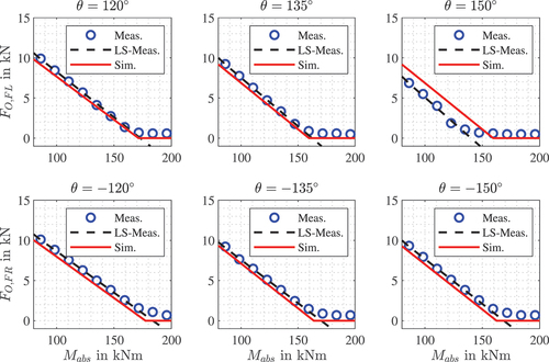
It can be observed that the measured outrigger forces are first decreasing linearly. Just before the measured contact force is reaching the value zero, the outrigger force is approaching some constant positive value. This value is exactly the weight of the outrigger plate that always remains in contact with the ground as described with Figure 6. Because the measured value never reaches zero, a linear approximation of the first segment is conducted by using the least-squares method. For comparing the measurement with the simulation, the critical moment of the unloaded outrigger is when the linear function is crossing zero. In simulation, the outrigger force is decreasing linearly until it becomes zero which is the time instant used for comparison to the measurement. After reaching zero, the simulated outrigger forces stays at this value.

For the comparison, the ‘critical moment’ $M_{\mathrm{crit}}$, at which the outrigger becomes fully unloaded, is listed in Table 1. This table displays the acting moment $M_{\mathrm{abs}}$ at the zero-crossing and the relative error defined by

Table 1. Prediction error w.R.t moment $\mathit{M}$.

Swing angle	$M_{\mathbf{crit}\mathbf{,}\mathbf{meas}}$ in $\mathit{kNm}$	$M_{\mathbf{crit}\mathbf{,}\mathbf{sim}}$ in $\mathit{kNm}$	${\epsilon }_{\mathbf{M}\mathbf{,}\mathbf{rel}}$ in $\mathrm{\%}$
$\mathit{\theta }={120}^{\circ }$	173.0	171.4	0.91
$\mathit{\theta }=-{120}^{\circ }$	184.0	177.5	3.52
$\mathit{\theta }={135}^{\circ }$	162.3	159.6	1.66
$\mathit{\theta }=-{135}^{\circ }$	170.3	163.9	3.78
$\mathit{\theta }={150}^{\circ }$	140.2	159.5	13.77
$\mathit{\theta }=-{150}^{\circ }$	168.8	162.5	3.74

(49) ${\epsilon }_{\mathrm{M},\mathrm{rel}}=\frac{\left|{\mathit{M}}_{\mathrm{crit},\mathrm{meas}}-M_{\mathrm{crit},\mathrm{sim}}\right|}{M_{\mathrm{crit},\mathrm{meas}}}.$(49)

A more intuitive representation is found in Table 2, comparing ‘critical ladder length’ $L_{\mathrm{crit}}$, both measured and in simulation. Due to the known relation between moment $M_{\mathrm{abs}}$ and ladder length $\mathit{L}$, these values can be easily obtained by interpolation. Here, the absolute error

Table 2. Prediction error w.R.t ladder length $\mathit{L}$.

Swing angle	$L_{\mathbf{crit}\mathbf{,}\mathbf{meas}}$ in $\mathit{m}$	$L_{\mathbf{crit}\mathbf{,}\mathbf{sim}}$ in $\mathit{m}$	${\epsilon }_{\mathbf{L}\mathbf{,}\mathbf{abs}}$ in $\mathit{m}$
$\mathit{\theta }={120}^{\circ }$	24.11	23.98	0.13
$\mathit{\theta }=-{120}^{\circ }$	25.02	24.49	0.53
$\mathit{\theta }={135}^{\circ }$	23.24	23.02	0.22
$\mathit{\theta }=-{135}^{\circ }$	23.90	23.37	0.53
$\mathit{\theta }={150}^{\circ }$	21.43	23.01	1.58
$\mathit{\theta }=-{150}^{\circ }$	23.77	23.25	0.52

(50) ${\epsilon }_{\mathrm{L},\mathrm{abs}}=\left|L_{\mathrm{crit},\mathrm{meas}}-L_{\mathrm{crit},\mathrm{sim}}\right|$(50)

is taken for comparison because it is directly the value of one controlled actuator that can be more easily interpreted.

For the first measurement at $\mathit{\theta }={120}^{\circ }$, the simulation predicts the unloaded outrigger from the measurements very well. The relative error is less than $1\mathrm{\%}$ that is resulting in an absolute error for the ladder length $\mathit{L}$ of only $0.13\mathrm{m}$. The measurements on the left side with $\mathit{\theta }=-{120}^{\circ }$ reveal that more load is needed to reach the critical moment when the outrigger is unloaded. One reason is the asymmetrical construction of the outriggers because they are not at the same $\mathit{x}$-position along the longitudinal axis. By considering this kinematics in the model, the same behaviour is achieved in simulation. However, the error is with $3.5\mathrm{\%}$ or $0.5\mathrm{m}$ slightly larger.

Both measurements at $\mathit{\theta }={135}^{\circ }$ and $\mathit{\theta }=-{135}^{\circ }$ confirm the previous observation. The critical moment $M_{\mathrm{crit},\mathrm{meas}}$ is larger for the measurement on the left side and the precision is slightly lower in that case. Overall, the precision of the prediction with errors less than $4\mathrm{\%}$ or respectively $0.55\mathrm{m}$ is satisfactory.

While the last measurement at $\mathit{\theta }=-{150}^{\circ }$ showed similar results as the measurements at other angles with errors less than $4\mathrm{\%}$ or respectively $0.55\mathrm{m}$, there is one clear outlier in the measurements at swing angle $\mathit{\theta }={150}^{\circ }$. It is the only time that the simulated critical moment is higher than the measured one. Also, the error between simulation and measurements is much larger in this case. The outlier at $\mathit{\theta }={150}^{\circ }$ exists because the outriggers were not setup explicitly before that specific measurement. During the operation, the distribution of the contact outrigger forces changed and were not symmetrical any more. Hence, the prediction of the unloaded outrigger is inaccurate. Nevertheless, when omitting this single outlier, the measurements are in general well represented by the simulation with the previously derived dynamic model.

5. Validation with dynamic measurements

So far, all simulations and measurements were conducted with slow velocities because of the following reasons: First, for the identification measurement it is more important to cover all swing angles than exciting dynamic oscillations. Second, for the validation of the fully unloaded outrigger, the ladder length is extracted where the actuator dynamics is usually slow. However, the presented model still aims to represent the dynamic oscillations of the system appropriately, when a typical dynamic excitation, e.g. by a high acceleration in the elevation angle, is applied to the ladder. This desired dynamic behaviour is approved in the following.

As the model shall be used for supporting the parametrization of the active damping control, the dynamic response to an impulse-type excitation is crucial. Therefore, the dynamic model of the ladder from (Densborn 2022) and the model of the chassis are connected to conduct some simulations that can be compared to dynamic measurements. For this purpose, the ladder is positioned to a swing angle of $\mathit{\theta }={90}^{\circ }$ and the system is excited by applying maximum speed in the elevation angle for a short time of 0.5 s. After the excitation, the outputs are measured during the free oscillation. The dynamic measurement in this section are not filtered at all because with the chosen excitation the structural oscillation is dominant compared to the measurement noise. Also, the original signal is not falsified like this.

Using the same excitation as in the measurements, the dynamic behaviour of the ladder can be simulated with the ladder model from (Densborn 2022). In Figure 10a, the vertical strain gauge $y_{\mathrm{vSG}}$ shows that the simulated oscillation of the ladder is nearly identical to the measured one. From that simulation, the external load $\mathit{u}={\left[\begin{array}{ccc}{F}_z& M_x& M_y\end{array}\right]}^{\mathrm{\top }}$ for the chassis model is derived with the moment $M_x$ around the longitudinal axis shown in Figure 10b being the most important load for the position $\mathit{\theta }={90}^{\circ }$. After applying this calculated load to the model of the chassis, all resulting outputs are simulated and compared to the measurements. In Figure 10c,d, two exemplary outputs are shown. With the chosen position and excitation, the torsional deformation ${\varphi }_1$ at the swing bearing and the force at the right, rear outrigger $F_{\mathit{O},\mathit{RR}}$ are the outputs of the most interest.

Figure 10. Simulation of the ladder dynamics with an impulse-type excitation (a) and the resulting load applied to the chassis (b). Then, validating the dynamic chassis model by comparing two important outputs in (c) and (d) to the measurements.

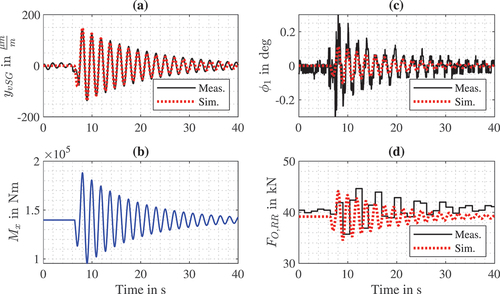
It is shown that the torsional deformation of the chassis ${\varphi }_1$ oscillates in the same frequency as the ladder and the oscillation decays in the same time. The lowest and most relevant eigenfrequency of the entire system is clearly the eigenfrequency of the ladder oscillation. In comparison, the computed eigenfrequency of the chassis model itself is around ten times larger than that. Therefore, all outputs are oscillated with the same frequency and damping as the ladder parts itself. In conclusion, the simulation represents the measurement of ${\varphi }_1$ well when omitting the measurement noise.

The measurement of the contact force $F_{\mathit{O},\mathit{RR}}$ reveal that the used wheel scales do not even fulfill the Nyquist – Shannon sampling theorem with the given eigenfrequency of the ladder. These sensors are usually used for static measurements and unfortunately its sampling time cannot be increased. However, the simulated force $F_{\mathit{O},\mathit{RR}}$ is clearly within the range of the measurements. The steady state offset differs by $2.9\mathrm{\%}$ and the relative error comparing the largest amplitude of the oscillation in both signals is $2.0\mathrm{\%}$.

6. Conclusion and outlook

A new dynamic model for a turntable ladder was derived by dividing the chassis into four parts reproducing a twisting and bending deformation. Also, the special support structure was considered that allows one outrigger to become completely unloaded. A parameter sensitivity analysis revealed that all parameters are identifiable, but their sensitivities are significantly different. Therefore, an identification approach with two steps is proposed that delivers better results than identifying all parameters at once. These optimized parameters are used in simulation that represent quasi-static measurements well. The simulation can recreate the point of time at which an outrigger becomes completely unloaded. However, it is important for predicting the unloaded outrigger that the outrigger setup is providing a symmetrical force distribution in the initial position.

Additionally, dynamic measurements after an impulse-type excitation were conducted. The ladder dynamics were simulated with a separate model from previous work calculating the resulting load acting on the vehicle chassis. Applying that load to the proposed dynamic model, the simulated outputs match the dynamic measurements well. The eigenfrequency of the overall system is clearly the same eigenfrequency of the ladder’s oscillations. The chassis stiffness is large, and hence, its eigenfrequency is not visible in the dynamic measurements anymore. However, the chassis model in combination with the ladder dynamics now represents the entire dynamics of the vehicle including all contact forces and flexible deformations of the chassis.

The presented results are promising, and the dynamic model will be useful to support the development work concerning the active oscillation damping control. Future work is to establish a simulation-based parametrization of the control system using the dynamic model of the overall turntable ladder. This approach possibly reduces the measurement effort significantly and therefore has potential to save costs. Also, the model of the support structure could provide interesting insights to the contact forces of the outriggers concerning structural safety and unloaded outriggers. Especially for dynamic trajectories close to the outreach limits, the impact of all dynamic effects onto the structural safety could be further examined in upcoming work.

Acknowledgments

This research has been conducted in close cooperation with Magirus GmbH, Ulm, Germany. The authors thank the industrial partner for many years of trustful partnership.

Disclosure statement

No potential conflict of interest was reported by the author(s).

References

- Andersson JAE, Gillis J, Horn G, Rawlings JB, Diehl M. 2019. CasADi: a software framework for nonlinear optimization and optimal control. Math Prog Comp. 11(1):1–36. doi: 10.1007/s12532-018-0139-4.
- Bestle D. 1994. Analyse und Optimierung von Mehrkörpersystemen. Berlin Heidelberg: Springer.
- Densborn S. 2022. Modellierung, Regelung und Trajektoriengenerierung für ein flexibles Mehrkörpersystem am Beispiel einer Feuerwehrdrehleiter. Düren, Germany: Shaker Verlag GmbH. doi: 10.2370/9783844086126.
- Densborn S, Sawodny O. 2021. Flexible multibody system modelling of an aerial rescue ladder using Lagrange’s equations. Math Comput Model Dyn Syst. 27(1):322–346. doi: 10.1080/13873954.2021.1918175.
- DIN EN 14043: 2014-04. 2014 Apr. High rise aerial appliances for fire and rescue service use - turntable ladders with combined movements - safety and performance requirements and test methods. DIN Deutsches Institut für Normung e.V.
- DIN ISO 8855:2013-11. 2013 Nov. Road vehicles - vehicle dynamics and road-holding ability - vocabulary. DIN Deutsches Institut für Normung e.V.
- Hasan S, Al-Hussein M, Hermann UH, Safouhi H. 2010. Interactive and dynamic integrated module for mobile cranes supporting system design. J Constr Eng Manag. 136(2):179–186. doi: 10.1061/(ASCE)CO.1943-7862.0000121.
- Horacio M. 2003. Nonlinear control systems: analysis and design. Hoboken, NJ: John Wiley & Sons.
- Jarzebowska E, Urbas A, Augustynek K. 2019. Analysis of influence of a crane flexible supports, link flexibility, and joint friction on vibration associated with programmed motion execution. J Vib Eng Technol. 8(2):337–350. doi: 10.1007/s42417-019-00186-1.
- Kemmetmüller W, Meiringer M, Platzgummer V, Kugi A. 2021. Optimale Abstützung eines mobilen Großraummanipulators. Automatisierungstechnik. 69(9):782–794. doi: 10.1515/auto-2021-0052.
- Ljung L. 1999. System identification: theory for the user (second edition). Upper Saddle River, NJ: Prentice-Hall.
- Majer CP. 1998. Parameterschätzung, Versuchsplanung und Trajektorienoptimierung für verfahrenstechnische Prozesse. Düsseldorf, Germany: VDI Fortschrittsberichte.
- Müller B, Rolle B, Sawodny O. 2022. Sensitivity analysis and fisher-information matrix for a dynamic model of a turntable ladder. IFAC-Papersonline. 55(27):172–177. doi: 10.1016/j.ifacol.2022.10.507.
- Nocedal J, Wright S. 2006. Numerical optimization. New York, NY: Springer New York.
- Pertsch A, Sawodny O. 2016. Modelling and control of coupled bending and torsional vibrations of an articulated aerial ladder. Mechatron. 33:34–48. doi: 10.1016/j.mechatronics.2015.11.009.
- Posiadala B. 1997. Influence of crane support system on motion of the lifted load. Mech Mach Theory. 32(1):9–20. doi: 10.1016/0094-114X(96)00044-4.
- Romanello G. 2018. Stability analysis of mobile cranes and determination of outriggers loading. J Engg, Design Technol. 16(6):938–958. doi: 10.1108/JEDT-05-2018-0084.
- Romanello G. 2022. A graphical approach for the determination of outrigger loads in mobile cranes. Mech Based Des Struct Mach. 50(3):767–780. doi: 10.1080/15397734.2020.1726184.
- Schmidt AP, Bitzer M, Imre ÁW, Guzzella L. 2010. Experiment-driven electrochemical modeling and systematic parameterization for a lithium-ion battery cell. J Power Sources. 195(15):5071–5080. doi: 10.1016/j.jpowsour.2010.02.029.
- Siciliano B, Sciavicco L, Villani L, Oriolo G. 2008. Robotics. London, England: Springer London Ltd.
- Skogestad S, Postlethwaite I. 2005. Multivariable feedback control: analysis and design. Chichester, West Sussex: Wiley.
- Trabka A. 2016. Influence of flexibilities of cranes structural components on load trajectory. J Mech Sci Technol. 30(1):1–14. doi: 10.1007/s12206-015-1201-z.
- Wanner J. 2024. Modellierung, Steuerung und Regelung für den Verteilermasts einer Autobetonpumpe. Düren, Germany: Shaker Verlag GmbH. doi: 10.2370/9783844093698.