Voice source, formant frequencies and vocal tract shape in overtone singing. A case study

Abstract

Purpose: In overtone singing a singer produces two pitches simultaneously, a low-pitched, continuous drone plus a melody played on the higher, flutelike and strongly enhanced overtones of the drone. The purpose of this study was to analyse underlying acoustical, phonatory and articulatory phenomena.

Methods: The voice source was analyzed by inverse filtering the sound, the articulation from a dynamic MRI video of the vocal tract profile, and the lip opening from a frontal-view video recording. Vocal tract cross-distances were measured in the MR recording and converted to area functions, the formant frequencies of which computed.

Results: Inverse filtering revealed that the overtone enhancement resulted from a close clustering of formants 2 and 3. The MRI material showed that for low enhanced overtone frequencies (F_E) the tongue tip was raised and strongly retracted, while for high F_E the tongue tip was less retracted but forming a longer constriction. Thus, the tongue configuration changed from an apical/anterior to a dorsal/posterior articulation. The formant frequencies derived from the area functions matched almost perfectly those used for the inverse filtering. Further, analyses of the area functions revealed that the second formant frequency was strongly dependent on the back cavity, and the third on the front cavity, which acted like a Helmholtz resonator, tuned by the tongue tip position and lip opening.

Conclusions: This type of overtone singing can be fully explained by the well-established source-filter theory of voice production, as recently found by Bergevin et al. [1] for another type of overtone singing.

Keywords:

• Formant clustering
• inverse filtering
• front cavity
• Helmholtz resonator
• tongue shape
• tongue tip
• area function

Introduction

Rendering melodies with overtones

The spectrum of a sustained vowel, whether sung or spoken, shows the amplitudes and frequencies of its harmonic partials. The frequency of the lowest partial f_o, – the fundamental, – determines the pitch of the vowel. The frequencies of the other partials – the overtones – occur at multiples of the f_o. Normally, they are not perceived individually. The spectral envelope determines the perceived vowel and voice quality. This is because our hearing system averages the spectral information in broad frequency bands – the critical bands of hearing.

Against this background, overtone singing comes across as a rather puzzling phenomenon. In this type of singing you hear a single voice produce two distinct pitches, a low-pitched drone and a whistle-like high tone, see e.g. [2]. The low-pitched tone is constant, while the high tone plays a series of harmonic partials or even melodies. An example can be found at t = 14.03 in [3].

Overtone singing was first described by Manuel Garcia [4]. Since then it has been analyzed by several voice researchers; for an overview, see e.g. [1]. More than half a century ago Smith and associates published the first investigation of a type of overtone singing, which was included in the religious ceremonies of certain Tibetan lamas [5]. Bloothooft and associates [6] applied acoustical analysis to examples provided by an experienced overtone singer. They concluded that enhanced overtones above 800 Hz may be interpreted as a clustering of formants two and three, achieved by a retroflex and rounded articulation. Bergevin and associates [4] recently published an exhaustive analysis of a type of overtone singing called Biphonic Tuvan throat singing. They analyzed the vocal tract shape using dynamic magnetic resonance imaging and calculated the associated formant frequencies in three overtone singers. Their results verified the earlier assumptions that also in Biphonic Tuvan throat singing the enhancing of a single spectrum partial is the acoustic result of clustering the second and third formants close to the enhanced overtone. They concluded that this type of overtone singing could be explained as a purely resonatory phenomenon.

As long as the pitch of the drone is kept constant, the ten lowest spectrum partials correspond to only a limited number of the tones constituting the scale typically used in western tonal music. For getting access to all pitches in these scales, it is necessary to use different drone tones. Our overtone singer subject explored this possibility when performing W A Mozart’s song Sehnsucht Nach der Frühlinge with overtone technique, where she shifts the pitch of the drone to get access to all pitches in the melody. A video of this performance, described in [7], shows her vocal tract in profile, recorded with magnetic resonance imaging at the Freiburg Institute of Musician’s Medicine and published on the website of the World Voice Day (world-voice-day.org). The present authors analyzed this MR documentation and complemented it with analysis of her voice source, modeling and synthesis; a condensed description of these analyses was recently published in Acoustics Today [8].^{1 2}

Background

Figure 1 shows a spectrogram of a passage of the video that includes shifts of the drone pitch. [2] Our overtone singer subject’s performance of the first bars of the song Sehnsucht Nach dem Frühlinge by W. A. Mozart is an interesting example [1], previously described and studied by Hefele and associates [2]. The timing and pitches of the first bars of the song are shown in the musical notation at the top of Figure 1(A).

Figure 1. (A) Score of the melody our overtone singer subject performed in overtone singing. (B) Partials are used for the melody tones (red lines) and the drone f_o (blue and black lines). (C) Wideband spectrogram of the performance (range 40 dB). Reproduced with the permission of the Acoustical Society of America.

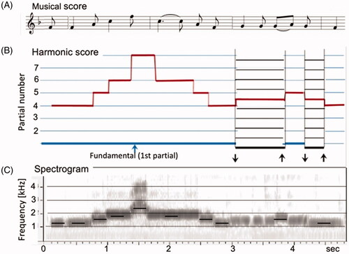
Section B illustrates how this melody was sung using the overtones of a drone. The vertical scale represents frequency, and the first eight harmonics are represented by the equidistant horizontal lines. Assuming that the singer selects a drone with a fundamental frequency, henceforth f_o, of 300 Hz, overtones will appear at integer multiples of 300 Hz: 600 Hz, 900 Hz, 1200 Hz, 1500, 1800 Hz, 2100 Hz, 2400 Hz. In other words, the frequencies of the overtones form ratios: (i) 1500/1200 = 1.25; (ii) 1800/1200 = 1.5; (iii) 2400/1200 = 2. These ratios correspond to musical intervals with the first note at 1200 Hz, major third, perfect fifth, and octave, respectively. Those intervals are sufficient to produce the notes of the first two bars.

However, the third bar uses the scale tone G. The series just mentioned does not provide an equally convenient choice for that note. Looking ahead to our overtone singer subject’s performance (part B) we see how she handled the situation: She lowered f_o to produce an overtone whose relation to 1200 is that of a major second, about 1.125! Our harmonic score includes that approach as illustrated below by a shift in f_o and the harmonics (thin and thick black lines).

The lower part of Figure 1(B) shows a spectrogram of our overtone singer subject’s overtone version of the song in terms of a wide-band spectrogram. The black short lines indicate the expected frequency values of the melody tones, assuming a drone with a f_o of 300 Hz. Note that these predictions agree with our overtone singer subject’s overtones rather well, even though the black marks slightly underestimate the observed values. The reason is that f_o of our overtone singer subject’s drones was slightly higher than our hypothetical 300 Hz.

The above illustrates the fact that overtone singing is a musical application of the harmonic structure of the overtones of periodic sounds. Overtone singers have developed a method of selecting and amplifying overtones to produce melodic sequences. This requires considerable precision of articulatory motor skills in time and frequency. Next, we will discuss how the needed amplification and selection may be achieved.

Acoustic theory

Amplification of single harmonic overtones

The envelope peaks of a vowel spectrum provide strong cues in the perceptual processing of vowels; it is the frequency locations of the formants that carry perceptually relevant information rather than their amplitudes; a change of the spectral tilt of a vowel spectrum, e.g. by applying a pre-emphasis of say +6 or −6 d B/octave changes the voice quality, while the phonetic vowel quality remains the same. Indeed, in the languages of the world, no sound systems use a phonological contrast between vowels in terms of merely spectral tilt difference. The reason is that formant amplitudes are predictable given the formant frequencies, so merely the overall spectrum tilt cannot be trusted with the task of carrying differences in meaning.

According to the classical source-filter theory of voice production, the envelope of a vowel spectrum, determining the amplitudes of the harmonics, is the sum of formant resonance curves, which are controlled by the shape of the vocal tract. Also contributing are certain more or less constant characteristics, such as radiation and the glottal source, which do not depend appreciably on articulatory activity [9]. We calculated spectrum envelopes of the tones in our overtone singer subject’s overtone singing using the equations given by Fant [9] (chapter 1.3 Analytical Constraints on the Composition of Speech Spectra). Thus, all transfer functions were derived as the sum of the envelopes for radiation, source, higher-pole correction, and formants. The shapes of the latter were accordingly computed from two numbers: The pole frequencies and the bandwidths of the formants. To calculate bandwidths the empirical formulas proposed by Fant were used: formants bandwidths are about 50 Hz for formant frequencies up to 2000 Hz and increase exponentially up to between 100 and 400 Hz at 4000 Hz [10]. Therefore, only the frequencies of the formants are needed for predicting the main characteristics of a spectrum envelope. This is illustrated in Figure 2, which shows three-line spectra and the cardinal resonance curve shapes for the first and second formants, F1 and F2.

Figure 2. Creating a “duplex formant” peak by moving two formants closer together. The schematic diagrams show F1 fixed at 600 Hz while F2 is shifted from 2150 Hz (left) to 1400 Hz (middle) to 650 Hz (left). Note the rightmost panel where F1 and F2 merge into a single peak, whose amplitude and the corresponding partial (arrow) are significantly enhanced. Reproduced with the permission of the Acoustical Society of America.

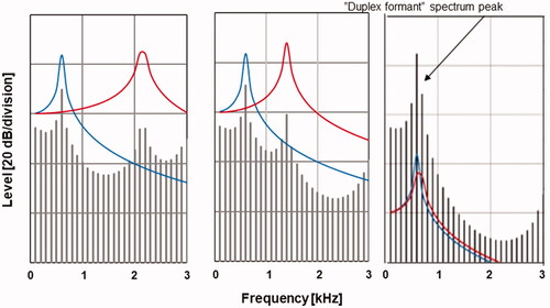
In the figure the amplitudes of the partials, and hence the spectral envelopes, were computed by the standard source-filter model [9] In the figure, F1 was fixed at 600 Hz while F2 was varied. The figure illustrates the fact that the amplitudes of two formants increase when the frequency distance between them is decreased. Therefore, when F1 and F2 approach almost identical frequencies (rightmost panel), creating a “duplex-formant,” a single spectrum peak with a very high amplitude is produced. In other words, the acoustic theory of voice production comprises a strategy for enhancing the amplitude of individual harmonics: Tune two formants to almost the same frequency, such that they create a duplex-formant!

These facts from the acoustic theory of voice production suggest an explanation of the overtone singing phenomenon. To test this possibility, measurements of formant frequencies were needed. We used two independent methods (1) analysing the sound by inverse filtering and (2) analysing the vocal tract shapes from the profile MR video of our overtone singer subject, and then estimating the frequencies of the vocal tract resonances, i.e. the formants, which were associated with the observed vocal tract shapes.

Measurements and modeling

Voice source characteristics: Inverse filtering

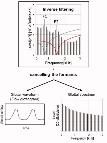
Inverse filtering is a classical method for analyzing the glottal sound source, and it has been extensively used for more than half a century, see e.g. [11–13]. The method, which is reliable for the typical f_o of adult male and female speech, is schematically illustrated in Figure 3. The basic idea is to remove the effect of the formants, so as to obtain a “residue” waveform representing the pulsating glottal airflow input signal of the vocal tract. By filtering the radiated vowel signal with filters representing the inverted (upside-down) version of the formant curves in Figure 3, the amplifying effect of the formant peaks is removed. Accurate tuning of each inverse filter ideally produces an output signal meeting two criteria: a waveform characterized by a ripple-free closed phase and a spectrum with an envelope void of troughs and peaks near the formant frequencies. In the waveform, referred to as the flow glottogram, the closed phase of the vocal fold vibration appears as a flat or sometimes somewhat tilted segment, surrounding quasi-triangular pulses that correspond to the open phase. A tilting closed phase can result from a piston motion of the glottal plane [14]. The steepness of the trailing end of the pulses, i.e. rate of flow decrease during the closing phase, varies systematically with vocal loudness. The peak-to-peak amplitude of the pulses varies with phonation type.

Figure 3. Schematic illustration of inverse filtering. Upper panel: input spectrum and frequency responses of inverse filters 1 and 2 (blue and red curves), which cancel the effects of F1 and F2 on the radiated spectrum. The bottom panels show the result of the inverse filtering in terms of the waveform or flow glottogram, and the spectrum of the voice source (left and right panels).

For analyzing formant frequencies, and also the phonatory characteristics of our subject’s overtone singing, an audio recording was made, where she produced a steady drone tone with a sequence of enhanced overtones, from the 4^th and up through the 10^th followed by a descending sequence down to the 4^th. The performance was picked up by an OM1 omnidirectional condenser microphone (Line Audio Design, Stockholm, Sweden, response 20–20000 Hz ±1 dB), held by the experimenter about 2 cm off the cheek and 6 cm from the lateral center of the lip opening, background noise 26 dB. It was connected to a Focusrite external soundcard, the output of which was fed via a USB contact to a PC and recorded by the Sopran software at a sampling rate of 44100 Hz.

The Inverse-filter module of the custom-made Sopran software [15] was used for the analysis. The frequencies and bandwidths of its inverse filters are tuned manually and the resulting waveform and spectrum are displayed in quasi-real-time. These frequencies and bandwidths are stored in a log file. The left panels of Figure 4 show a typical example, where the frequency of the enhanced overtone, henceforth F_E, was 1510 Hz. The flow glottogram shows an almost perfectly ripple-free closed phase with a slight negative tilt and the envelope of the corresponding spectrum is smooth up to and beyond F_E.

Figure 4. Left three panels: (A) Radiated spectrum for an F_E of 1490 Hz; (B) Flow glottogram and (C) spectrum of the associated voice source. Middle panels: Closed quotient (D) and normalized amplitude quotient (E) as functions of F_E; triangles and diamonds refer to data from the ascending and the descending sequence of overtones, respectively. Rightmost panel: The lowest three formant frequencies F1, F2, and F3, used in the inverse filtering and plotted as a function of F_E.

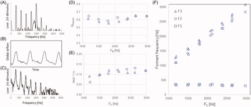
The two graphs in the center of the figure shows two aspects related to phonation type, the closed quotient Q_Closed, defined as the relative duration of the closed phase, and the normalized amplitude quotient NAQ, defined as the ratio between the peak-to-peak pulse amplitude and the negative peak amplitude of the derivative of the flow glottogram, or maximum flow declination rate. The variation with F_E is small and systematic, and the data points from the ascending and the descending F_E sequences are similar, suggesting well-controlled phonation. The mean Q_Closed is close to 0.6 and the mean source spectrum slopes 8.7 dB/octave. The mean level difference between the lowest two source spectrum partials (H1–H2) was −2.6 dB, which can be compared with +2.1 dB found for untrained female speakers [16]. The mean NAQ was close to 0.12, while 0.15 has been found for untrained female speakers [17]. These results suggest that our overtone singer subject used a rather high degree of glottal adduction in her overtone singing.

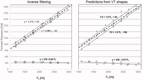
The frequencies of the lowest three formants used for the inverse filtering are plotted against F_E in the rightmost panel of Figure 4. F2 and F3 surround F_E closely, while F1 is close to the 300 Hz f_o of the drone and shows a slight trend to decrease with increasing F_E. The inverse filtering thus supported the assumption that F1 was tuned to a frequency just above the f_o of the drone, and that F2 and F3 formed a formant cluster centered at F_E, thus supporting the assumption that our overtone singer subject’s overtone singing is produced with a “duplex-formant” technique.

Analyses: Formants and cavities in overtone singing

As formant frequencies are determined by the shape of the vocal tract, another possibility of testing the “duplex-formant” hypothesis was to derive vocal tract shapes from a dynamic MR documentation of our overtone singer subject’s vocal tract during overtone singing. Thus, the aim of this section is to describe the vocal tract shape for each F_E (analysis) and then to calculate the formant pattern she used in her overtone singing (synthesis). Of particular interest is to see whether the “duplex-formant” effect would crop up and if there is a reasonable numerical agreement between its center frequency and the observed FE:s. If perfect matches are obtained, we will be justified in concluding that our model – essentially based on the classical source-filter theory of Fant [9] and Stevens [18] – is sufficient to explain the overtone singing phenomenon.

A standard way used to analyse vocal tract shapes is to divide the vocal tract into cross-sections, measure the area and the length of each section and then plot the areas as a function of the section’s position along the vocal tract. Such a diagram is known as the (cross-sectional) area function, allowing calculation of the formant frequencies of any given vocal tract shape.

Data sources

Our observations come from three recordings made on separate occasions: (i) the audio recording mentioned above, used for the inverse filtering analyses; (ii) a dynamic MRI video showing how she formed her vocal tract as she changed F_E; (iii) a frontal-view video of the lip opening. In all these three recordings our overtone singer subject produced the same series as in the audio recording (i). For documenting the lip opening in the frontal video, distance measurements were obtained from a ruler with an mm scale next to the lip opening. The dynamic MR video Naturtonreihe in Zungentechnik, produced at the Freiburg Institute of Musician’s Medicine (https://youtu.be/-jKl61Xxkh0), shows our overtone subject’s entire vocal tract in mid-sagittal lateral profiles. In the MR images, distance calibration was based on known distances between fixed anatomical landmarks on the singer’s skull.

Area functions and formant frequencies

Area functions

Back cavity

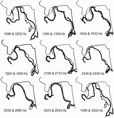
For each of the tones, an MR frame was selected near the middle of the duration of the F_E. The contours of the visible structures were then traced as illustrated in Figure 5. To compare tracings from different frames it was necessary to correct for slight head movements. The tracings were therefore rotated and translated to be placed in a common coordinate system anchored in fixed anatomical landmarks. The full set of tongue shapes is presented in Figure 5.

Figure 5. Tracings of the lateral midsagittal articulatory profiles were observed in the MR images of the subject while producing the indicated F_E in the ascending and descending sequences. Reproduced with the permission of the Acoustical Society of America.

As mentioned, area functions can be used as input for calculating the associated vocal tract resonance characteristics. As the MR video was dynamic, it allowed our overtone singer subject to perform overtone singing in her habitual way and we could follow how she changed her articulation as she shifted F_E. On the other hand, the movie offered no volumetric vocal tract data. In such cases, an indirect method can be used. Direct measurements of cross-sectional areas have been reported in the literature and have been shown to vary in lawful ways as a function of location in the vocal tract and the cross-distance between a fixed contour (e. g., palate, pharyngeal wall) and the articulator (e. g., the tongue body). The result is empirical distance-to-area rules, i.e. formulas that return estimates of areas from known cross-distances at given vocal tract locations. These rules will be specified below.

Lacking direct measurements for our overtone singer subject, we used data tabulated in Appendix E3: Articulatory measurements in Christine Ericsdotter’s doctoral dissertation [19]. Her study contains detailed analyses of MR images of Swedish vowels. It is a rich source of precise and quantitative information including mid-sagittal cross-distances and cross-sectional areas along the vocal tract. This data set was obtained from sagittal, coronal, and axial MR images of two repetitions of eleven vowels produced by a male and a female speaker.

Measurements were made with the aid of a system of gridlines that indicate the positioning of the image “slices” and define vocal tract locations relative to fixed anatomical landmarks. Figure 6(A) shows the grid used by Ericsdotter, here fitted to one of our overtone singer subject’s vocal tract profile images using the corresponding anatomical landmarks, such as the maxilla and the back pharynx wall.

Figure 6. (A) Shows the system of gridlines used for deriving the vocal tract cross-distances needed to represent the shape of the vocal tract as a cross-sectional area function. Calibrated in real mm it is used to measure the width of the vocal tract along each gridline and to construct a vocal tract midline as a piecewise linear contour passing through the midpoints of the width segments (indicate by white dots and connecting lines). In (B) these width segments have been modified in length and rotated around their midpoints so as to be approximately normal to the midline. Their lengths, so modified, now define the cross-distances (i e between tongue and back pharynx wall/palate) needed to calculate cross-sectional areas using the linear distance-to-area rules.

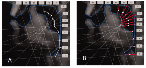
To represent a given vocal tract shape as an area function, for the lateral profile of every vowel token, the width of the vocal tract is first measured along each of these gridlines. By definition, the vocal tract midline crosses that width segment at the midpoint. In Figure 5 the midpoints are indicated by white dots and connected by straight lines.

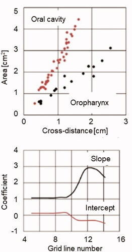
Ericsdotter derived all cross-sectional areas from the coronal and axial slices. One of the aims of her work was to investigate how well measured cross-sectional areas can be estimated from the corresponding vocal tract width. The cross-distances for the profile in Figure 6 are shown as red segments. Ericsdotter found that, in most cases, it is possible to use a power function – A = αd^β – to predict cross-sectional areas (A) from cross-distances (d) with sufficient accuracy. Her data set allowed us to formulate our own d-to-A (distance-to-area) rules. We found that, within the variation range of interest here, linear equations could also be readily fitted to all her female data.

Table 1 lists slopes, intercepts, and R2 values (the correlation coefficient squared) for this description. The “location” column specifies the distance of the gridline intersection from the front end, i.e. the upper incisors, as measured along the upper/posterior contour, i.e. the palate/pharynx wall. As can be seen, this method results in consistently high R2 scores.

Table 1. Slopes and intercepts were used to derive estimates of the subject’s cross-sectional areas from measured cross-distances.

Location [cm]	Gridline #	Slope	Intercept	R2
5	11	2.34	−0.49	0.88
7	10	2.85	−0.33	0.96
7.8	9	2.85	−0.33	0.96
8.7	8	1.92	−0.31	0.96
9.4	7	1.42	−0.15	0.92
10.2	6	1.12	0.15	0.85
10.8	5	1.12	0.15	0.85
11.7	4	1.07	0.12	0.94
13	3	1.07	0.12	0.94
14.2	2	1.07	0.12	0.94

The high R2 values give an indication of the predictive quality of the linear model. The Location column lists gridline distance from the front end of the vocal tract (upper incisors) to the upper/posterior contour (palate/back pharynx wall) with any given grid line. The gridline numbers, starting from the larynx, are those shown in Figure 6. Reproduced with the permission of the Acoustical Society of America.

In Figure 7 curved lines are used to highlight the fact that the slope and intercept numbers vary smoothly along the vocal tract (equivalently, as a function of grid number). We take this pattern of continuity to reflect the fact that the geometry of the vocal tract also changes smoothly.

Figure 7. Upper graph: Examples illustrating the linearity of the d-to-A rules. Cross-sectional vocal tract area as a function of the cross-distance in the oral cavity (gridlines 9–11) and oropharynx (5–8). Lower graph: Highlight of the smooth variation of slopes and intercepts listed in Table 1.

The selected MR frames confirmed that, at the low-frequency end of the overtone singing sequence, our overtone singer subject used a raised and retracted tongue tip. As she shifted to higher F_E there was less and less retraction. Thus, the tongue tip position along the palate was moved systematically with F_E; the higher the frequency, the more anterior the place of articulation, (see Figure 6). As F_E was increased the length of the constriction also became more extensive. As a result, the tongue configuration changed from an apical, fronted into a more dorsal, posterior articulation.

The upper panel of Figure 7 shows distance/area correspondences pooled for the gridlines in the oral cavity and in the oropharynx. The linear nature of the data is evident. The lower diagram demonstrates that the slopes and intercepts (Table 1). As mentioned, the smooth variation of these values along the vocal tract length axis seems to mirror the smoothly varying cavity shapes.

Front cavity

In post-dental and retroflex consonants the tongue tip is retracted and raised towards the hard palate [20,21]. This gesture adds a subapical space to the front cavity that has a significant effect on the formant pattern. The literature indicates that the front cavity including the subapical volume can be modeled acoustically as a Helmholtz resonator, the neck of which is the lip [17]. The volume of such a resonator is crucial to its resonance frequency but impossible to accurately determine from a vocal tract MRI profile.

An article by Granqvist and colleagues [22] reports relevant data on subapical volumes for dental and retroflex stops. This study employed electropalatography, described in detail in the article, to determine place of articulation. The tongue’s contact on the palate was sampled every 10 msec. Volumes were estimated from the front cavity resonance. To increase the accuracy of those measurements, pulse excitation of the front cavity was added and recorded with the speech signal. The excitation signal was a pulse, 50 Hz repetition rate, obtained from an earphone and attached to a thin, 5 cm long, plastic tube, the resonances of which were compensated for by inverse filtering the input excitation signal. The tube’s open end was placed in the subject’s front cavity. The audio signal picked up by a microphone a few centimeters in front of the subject’s lips contained both the subject’s voice and the front cavity’s response to the pulse signal excitation. The female subject sealed her lips around a brass tube and held it firmly against her teeth. To keep the jaw position constant, it was fixed by a 5 mm bite-block placed between the first molars. On the assumption of the system behaving as a Helmholtz resonator, the investigators were able to make estimates of the volume of the front cavity; the procedure with constant area and length of the lip tube allowed accurate determination of the frequency of the front cavity resonance for each time sample. The results showed that the front cavity volumes, ranging between 2 cm³ and 11 cm³, varied with the place of articulation along approximately straight lines.

We decided to parallel the approach of Granqvist et al. in dealing with the front cavity. Our procedure is illustrated in Figure 8. From the MR images, we estimated the length of the lip section. The place of articulation was located at the end of the constriction. Data on the lip opening areas were obtained from the frontal-view video images; the sides of a rectangle were fitted to the innermost corners of the lips and the uppermost and lowermost tangents of the upper and lower lips, respectively. Measures of height (h) and width (w) of opening were then fed into the following formula for the lip opening area (A) [23]: $$A\mathrm{ }=hw{\left.\left(\mathrm{ }\frac{p}{p+1}\right.\right)}^{}$$

Figure 8. Illustration of the method used for measuring the front cavity, see text.

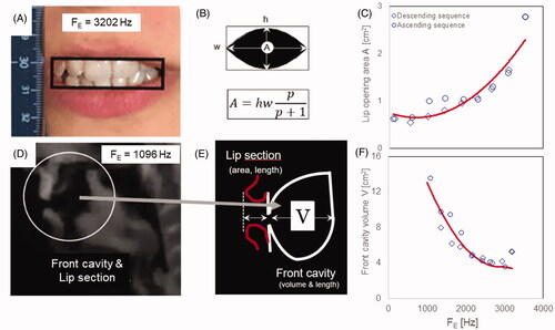
This expression follows from representing upper and lower lip contours by a power function whose exponent (p) determines their curvature. A value of p = 2 implies that lip openings differ from rectangles with identical h and w by a factor of 0,67. Empirical data confirm that estimate [24]. The upper rightmost panel of Figure 8 shows thus estimated lip opening areas as a function of F_E in our overtone singer subject’s front video recording. The curve illustrates a precise and systematic variation.

Given these lip measurements and F_E we used the standard Helmholtz formula to infer volumes that would provide perfect matches with observed F_E s. $$f\mathrm{ }=\mathrm{ }\frac{c}{2\mathrm{\Pi }}\mathrm{ }\sqrt{{\left.\left(\mathrm{ }\frac{A}{l\mathrm{*}V}\right.\right)}^{}}$$

The result of the calculations is presented in Figure 9. Volume values are here plotted against the place of articulation for overtone singing and for two test words from the Granqvist [22] study in which the retroflex consonants are preceded by vowels with palatal and pharyngeal constrictions, respectively, and therefore similar to the endpoints of the overtone singing sequences. At low F_E:s, produced with the retracted place of articulation, the inferred volumes for overtone singing overlap with the [ha:ɖɛ] data cluster, at high frequencies with the [hy:ɖɛ] data.

Figure 9. Front cavity (FC) volume as a function of place of articulation, comparing volumes derived from our overtone singer subject’s overtone singing (blue circles) with those reported by Granqvist and collaborators [17] during the closure of the retroflex consonants in/hy:ɖe/and/ha:ɖe/(black and red circles).

Formant frequencies

As evident from Figure 5, vocal tract profiles share the following two characteristics. They all exhibit a three- or four-tube configuration – schematically, front cavity + constriction + back cavity + (for low F_E pharyngeal) constriction. There is also the common feature of a narrow constriction area – a fact that implies that there was only limited acoustic interaction between front and back cavities and thus justifying our treatment of the front cavity as a separate Helmholtz resonator.

The articulatory information reviewed so far takes us to the next step: Deriving the area functions and their formant patterns. First, a comment on our hybrid approach – hybrid in the sense that, for the constriction and the back cavity, we used the standard method based on our MR observations and distance-to-area rules. However, this approach runs into difficulties when the front cavity includes an extra subapical cavity under the tongue blade. To get around this problem we chose to represent the oral part of the front cavity by a single section, whose length was obtained from the MR images and whose area equaled the section’s calculated volume divided by the front cavity length. The opening area and the length of the lips were given by the video and the MR measurements.

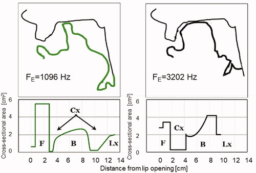
Applying these procedures, vocal tract area functions were established for the entire set of 13 MR profiles, 7 from the part with ascending F_E:s and 6 from the following part with descending F_E:s. Figure 10 shows the MR tracings and the corresponding derived area functions obtained for the lowest and the highest F_E:s.

Figure 10. Upper panels: MR tracings of the lowest and the highest F_E (left and right panels). Lower panels: schematic illustration of the corresponding front cavity, constrictions, back cavity and larynx (F, Cx, B, and Lx, respectively) of the corresponding derived area functions.

Transfer functions

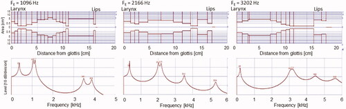
To calculate formant frequencies we used the Wormfrek software, a program written by Johan Liljencrants and described in detail in [25]. It computes the transfer functions (including lip radiation) of the input area tables, displays the transfer function, and tabulates the formant frequencies assuming losses according to Fant [26]. Sample results are shown in Figure 11. The panels of the top row present the area functions of F_E = 1096, 2166, and 3202 Hz. Spectrum envelopes for these tokens are seen on the second row. Note the “duplex-formants” – that is, the close proximity of F2 and F3 for F_E = 1096 Hz and 2166 Hz, and, for F_E = 3202, their merging into a single peak.

Figure 11. Derived area functions and corresponding computed transfer functions (upper and lower series of panels) for the indicated F_E.

The complete picture of the simulations is summarised in Figure 12. We note that for both F2 and F3 the data points line up along straight lines with slopes close to 1,0. Intercepts tell us that the formants are separated, but that gap is sufficiently narrow to produce a significant enhancement of the spectral envelope, illustrated in Figure 11, which the overtone singer knows how to take advantage of.

Figure 12. The lowest three formant frequencies used in the inverse filterings and produced by the area functions (left and right panels) are plotted as a function of F_E. Dotted lines and equations refer to the trendlines. Dashed lines represent the identity of formant frequency and F_E.

Discussion

Previous research

The “duplex-formant” hypothesis attributes the phenomenon of overtone singing to vocal tract filtering. In addition, inverse filtering results strongly suggested that the type of overtone singing analyzed used a special type of phonation: The flow glottograms exhibited a longer-than-normal closed phase, and the values of the NAQ parameter were low. This suggested that our overtone singer subject used a slightly firmer vocal fold adduction in her overtone singing as compared with what is typically found in untrained female’s conversational speech. These findings replicate and extend some previous investigations of overtone singing. Thus, Bloothooft et al. [6] suggested formant clustering as an explanation of the enhanced overtone and observed signs of an extended closed phase of the vocal fold vibrations. Kob & Neuschaefer-Rube [27] and Kob [27] used impedance measurements in an analysis of a type of overtone singing called sygyt. They and Hefele et al. [7] interpreted the boosting of the overtones as the result of clustering of formants 2 and 3. Kob [28] hypothesized that this clustering could be the result of combining a longitudinal resonator with a Helmholtz resonator in front of a palatal constriction, a hypothesis confirmed by the present study.

Klingholz [29] analyzed the overtones of a male singer by means of LPC. This singer used a drone f_o of 127 Hz and enhanced its partials 2, 3, 4, and 5. The analysis showed an unusually high peak at the enhanced partial, which was assumed to reflect an abnormally narrow formant bandwidth, possibly resulting from a coupling between the vocal tract with the vocal fold mechanism. A problem with this explanation is that formant bandwidth values mainly depend on heat loss, viscous loss, radiation loss, and glottal loss [30]. Therefore, they are less likely to be under the direct control of a speaker/singer. In addition, our inverse filtering results clearly rule out the existence of a laryngeal mechanism that selectively amplifies individual partials.

The spectra published in the study by Bergevin and associates [1] of biphonic Tuvan throat singing differ in certain respects from those analysed in the present study; first, the strongest overtone was much more enhanced than in our overtone singer subject’s overtone singing; second, the spectrum envelope showed several sharp dips; and third, the fundamental was between 20 and 40 dB weaker than the second partial. Also, the articulatory configurations differed from those of our overtone singer subject, lacking a narrowed lip opening and containing not only an elevated and retracted tongue tip, but for some F_E values also a vocal tract narrowing in the velopharyngeal region. Thus, not unexpectedly, the Biphonic Tuvan throat singing is produced with a vocal technique differing from the one our overtone singing subject uses.

No general conclusions can be drawn from the present single-subject study of polyphonic overtone singing. Instead, we conclude that our analysis of our subject’s overtone singing and previous investigations of sygyt and some other types of overtone singing provide strong and convergent evidence that both the selection and the observed significant enhancement of a specific overtone of the drone can be explained by the “duplex-formant” phenomenon, i.e. the tuning of two formants to frequencies close to the frequency of the enhanced overtone.

Overtone singer’s path in articulatory space

Our results raise the question of how the motor control of overtone tuning might be organized. As mentioned above, the articulatory profile for F_E = 1096 Hz resembles the raised tongue blade of retroflex consonants. There is also a narrow pharyngeal constriction typical of [a]-like vowels and pharyngealized consonants [31]. The vocal tract shape for F_E = 3202 Hz, on the other hand, has an [i]-like, “palatalized” tongue shape. In Table 2 we suggest that, schematically, these cases can be seen as opposites.

Table 2. Schematic classification of the vocal tract shapes of the extremes of the overtone sequence.

FE	Front cavity	Constriction	Back cavity	Larynx tube
1096	Large	Short	Narrow	Low
3202	Small	Long	Wide	High

Reproduced with the permission of the Acoustical Society of America.

To elaborate on this visual impression, we used our measurements to examine how the categories of the above table change during the overtone sequences. We selected the data for lip opening area, length of palatal constriction, larynx height, front cavity volume, and pharynx width and plotted them against overtone frequency. Figure 13 shows the result. To highlight the continuity of the movements we connected the points by hand. It would appear that the values of each individual articulatory dimension are aligned along smooth contours running between its extreme values.

Figure 13. Articulatory parameters are derived from the area function tables and plotted as functions of F_E. The manually drawn curves illustrate the continuous variation of the articulatory parameters with F_E. Reproduced with the permission of the Acoustical Society of America.

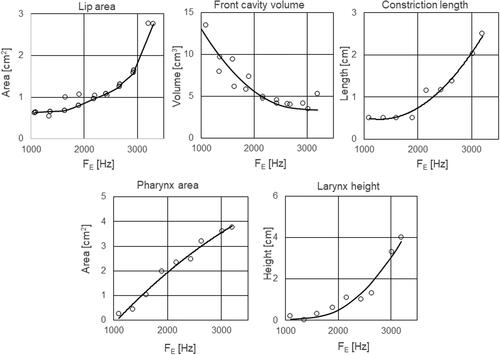
A rough description of the present set of overtone’s paths through articulatory space would be to say that vocal tract shapes are located along a trajectory that runs between a strongly retroflex and pharyngealized [a] and an [i]-like, palatalized tongue profile.

Conclusions

• Inverse filtering confirmed the use of duplex-formants in amplifying and selecting individual harmonics. Further, the voice source remained consistently stable across the entire corpus of analyzed data, thus implying that it plays no role in the process of amplification and selection. Phonation type was slightly more pressed than in conversational speech, which tends to boost high-frequency harmonics. F2 and F3 were tuned to frequencies close to and on each side of that of the enhanced partial, thus producing a “duplex-formant.”

• The resonance properties of the estimated vocal tract shapes were all found to exhibit F2 and F3 in close proximity, thus providing independent support of the concept of a “duplex-formant.” This proximity was achieved by a vocal tract shape containing two or three major cavities separated by constrictions. The front cavity acts as a Helmholtz resonator. Adjustment of its volume produces resonance with frequencies between 1000 and 3200 Hz. In the posterior region either the tongue constriction or the pharynx tune the other member of the duplex formant.

• The lateral profiles of the vocal tract shape revealed an articulatory continuum that emerged the showed a certain complementarity: For the lowest pitch, there was a large front cavity, a retracted, “hyper-retroflex” tongue tip/blade, a maximally low larynx, and a narrow pharyngeal constriction. For the highest pitch, the vocal tract configuration showed a small front cavity, a palatalized [i]-like tongue shape, a raised larynx, and an enlarged pharyngeal cavity. Acoustically this articulatory continuum has the interesting property of generating one anterior and one posterior formant of almost identical frequencies in the range between 1000 and 3200 Hz.

• This complementary organization of motor control seems to be the mechanism that exploits vocal tract physics, to deliver duplex formants for overtone singing.

Disclosure statement

No financial interest or benefit has arisen from the direct applications of this research.

Notes

1 Following the publication rules of that journal, no detailed specifications of methods were included in that report. The present article provides a full account of the investigation.

2 It is no accident that our musical scales and the intervals between them are closely related to the harmonic structure of periodic sounds. Actually, this property of periodic sounds plays is crucial to our perception of consonance and dissonance phenomenon [3,4].

References

- Bergevin C, Narayan C, Williams J, et al. Overtone focusing in biphonic tuvan throat singing. eLife. 2020;9:e50476.
- Zemp H, Hai TQ. Recherches expérimentales sur le chant diphonique. Cahiers D’ethnomusicologie. 1991;4(1):27–68.
- Hai TQ. Sound example available from: https://www.youtube.com/watch?v=Eysu0odOips
- Garcia M. 1847. Traité complet de l’art du chant. Paris: Troupenas.
- Smith H, Stevens K, Tomlinson R. On an unusual mode of singing by certain Tibetan lamas. J Acoust Soc Am. 1967;41(5):1262–1264.
- Bloothooft G, Bringmann E, van Cappellen M, et al. Acoustics and perception of overtone singing.? J Acoust Soc Am. 1992;92(4 Pt 1):1827–1836.
- Hefele AM, Eklund R, McAllister A. Polyphonic overtone singing: an acoustic and physio- logical (MRI) analysis and a first-person description of a unique mode of singing. In: Mattias Heldner (ed.): Proceedings from Fonetik. Sweden: Stockholm University; 2019. p. 91–96.
- Sundberg J, Lindblom B, Hefele A-M. One singer, two voices. Acoust Today. 2021;17(1):43–51.
- Fant G. 1960. The acoustic theory of speech production. The Hague: Mouton.
- Fant G. 1972. Vocal tract wall effects, losses and resonance bandwidths. In: Quarterly progress and Status Report. Stockholm: Department of Speech Hearing and Music, KTH.
- Rothenberg M. A new inverse-filtering technique for deriving the glottal airflow waveform during voicing. J Acoust Soc Am. 1973;53(6):1632–1645.
- Holmberg EB, Hillman RE, Perkell JS. Glottal airflow and transglottal air pressure measurements for male and female speakers in soft, normal, and loud voice. J Acoust Soc Am. 1988;84(2):511–529.
- Sundberg J, Gauffin J. Waveform and spectrum of the glottal voice source. In: B Lindblom, S Öhman, editors. Frontiers of Speech Communication Research. London: Academic Press; 1979. p. 301–320.
- Hertegård S, Gauffin J, Karlsson I. Physiological correlates of the inverse filtered flow waveform. J Voice. 1992;6(3):224–234.
- Granqvist S. Sopran. Software available from www.tolvan.com; 2021.
- Garellek M, Samlan R, Gerratt BR, et al. Modeling the voice source in terms of spectral slopes. J Acoust Soc Am. 2016;139(3):1404–1410.
- Alku P, Bäckström T, Vilkman E. Normalized amplitude quotient for parametrization of the glottal flow. J Acoust Soc Am. 2002;112(2):701–710.
- Stevens KN. 1998. Acoustic phonetics. Cambridge (MA): M.I.T. Press.
- Ericsdotter C. 2005. Articulatory-acoustic relationships in Swedish vowel sounds Doctoral dissertation. Stockholm University.
- Dixit RP. Lingotectal contact patterns in the dental and retroflex stops of Hindi. J Phon. 1990;11:291–302.
- Krull D, Lindblom B. Coarticulation in apical consonants: acoustic and articulatory analyses of Hindi, Swedish and Tamil. In: Quarterly progress and Status Report. Vol. 2. Stockholm: Department of Speech Hearing and Music, KTH; 19962. p. 73–76.
- Granqvist S, Sundberg J, Cortes EE, et al. The front and sub-lingual cavities in coronal stops: an acoustic approach to volume estimation. In: Proceedings of the 15th international congress of phonetic sciences. Barcelona; 2003. p. 941–944.
- Lindblom B, Sundberg J. Acoustical consequences of lip, tongue, jaw and larynx movement. The Journal of the Acoustical Society of America. 50:4, 1166–1179. Reprinted in Kent R D, Atal B S & Miller J L (eds): Papers in Speech Communication: Speech Perception. New York: Acoust Soc Am.; 1971/1991. p. 329–342.
- Fromkin V. Lip positions in American English Vowels. Lang Speech. 1964;7(4):215–225.
- Liljencrants J, Fant G. Computer program for vocal tract-resonance frequency calculations. In: Quarterly progress and Status Report. Stockholm: Department of Speech Hearing and Music, KTH; 1975:4, 15–20.
- Kob M, Neuschaefer-Rube C. 2003. Acoustic analysis of overtone singing. In: Proceedings of the 3rd International Workshop MAVEBA 2003, 187-190 187–190.
- Kob M. Analysis and modelling of overtone singing in the sygyt style. Appl Acoust. 2004;65(12):1249–1259.
- Klingholz F. Overtone singing: productive mechanisms and acoustic data. J Voice. 1993;7(2):118–122.
- Flanagan JL. 1965. Speech analysis synthesis and perception., 1st ed, New York: Springer.
- Ladefoged P, Maddieson I. 1986. The sounds of the world’s languages. Oxford: Blackwell.