Euro area monetary policy transmission in Estonia

Abstract

This paper studies the effect of a monetary policy shock in the euro area on the main Estonian economic and financial variables between 2000 and 2012. Using a standard structural vector autoregression (SVAR) model we find strong and persistent effects on Estonian GDP, private consumption, corporate investment, and imports. A monetary policy shock also has strong and sluggish effects on the housing loan and consumer credit interest rates. The estimated reaction of Estonian GDP and the GDP deflator-based inflation rate is about four times stronger than the reaction of euro area-wide aggregates. The strength of the impact depends on the inclusion of the data from the years of the recent financial and economic crisis.

Keywords:

• Estonia
• euro area
• monetary policy
• SVAR

JEL classification codes:

• E32
• E52
• C32

1. Introduction

Understanding the effects of monetary policy shocks across the euro area countries plays a crucial role in policy making and in communicating the policy strategy. More so because the recent financial and economic crisis might have affected the transmission of monetary policy shocks. In this paper we ask how monetary policy shocks in the euro area affect the main Estonian economic and financial variables. We also look at how the recent financial and economic crisis and possible extreme observations in the data affect the results.

The estimated structural VAR model shows that a negative monetary policy shock in the euro area of one standard deviation (an increase in the 3-month Euribor of 22 basis points (bp)) has a strong impact on the Estonian economy.

• Estonian GDP follows a hump-shaped response, reaching the lowest point of –1.8% after 8 quarters and converging very slowly to the baseline. Private consumption and corporate investment also contract strongly, peaking at 2.7% and 5.2% respectively, and converging slowly.

• The GDP deflator-based inflation rate initially increases by 0.4 percentage points (pp), but then falls to –0.6 pp after 3 quarters and converges back to the baseline after 3 years.

• Exports and imports shrink by 2.2% and 4.2% respectively. Employment falls after 10 quarters by 1.3% and real wages by 1.2%.

• All Estonian interest rates increase over several quarters, before converging back to the baseline. The Estonian money market interest rate (the 3-month Talibor) rises on the impact by 11 bp and peaks around 34 bp after a year. Housing loan and consumer credit interest rates react sluggishly, reaching the peak between three and four quarters after the initial shock. The business loan interest rate reacts little, by a maximum of 13 bp. The effect of the business loan interest rate is small, especially when compared to that of the housing loan and consumer credit interest rates, which increase by 38 and 40 bp respectively.

• Euro area GDP falls persistently. The GDP deflator-based inflation rate drops the quarter after the shock, and converges fast. The reaction of Estonian GDP and the GDP deflator-based inflation rate is about four times stronger than that of the euro area-wide aggregates. The Estonian money market interest rate, the three-month Talibor, reacts about twice as strongly as the euro area money market interest rate, the three-month Euribor.

Our evidence suggests that Estonian economic and financial data are volatile at least partly because of internal amplification. By construction the identified monetary policy shock is identical for the euro area and for Estonia but the money market and the three loan type specific interest rates amplify the reaction of economic variables.¹ Not only does the Estonian money market interest rate increases together with the three-month Euribor at the quarter of the shock, but it continues to increase while the euro area interest rate converges in five quarters. Moreover, housing loan and consumer credit interest rates increase by about the same magnitude as the Talibor. The reaction of the business loan interest rates is more muted than that of the Estonian money market interest rate.

During the last 13 years, Estonian data have high variance and include several extreme values and possible outliers. The residuals are not well described by a standard normal distribution – they have fat tails and are skewed. As a robustness exercise, we remove some of the variance in the residuals by including dummies. First, we find that after adding dummies in the Estonian equations, the impact of a monetary policy shock in the euro area on the Estonian variables decreases. By adding dummies only to the period of the global financial and economic crisis from 2007Q3 to 2010Q2, we see the strong impact of the crisis as, for example, the reaction of GDP is half what it is in the benchmark results when the crisis years are removed from the data, with Estonian GDP dropping by only 0.8%. We also estimate models for shorter time periods to see which years cause the changes in the transmission mechanism. Using the rolling time-window approach we confirm the results from the approach using dummies. We observe a strong impact from the crisis period, especially the years 2008 and 2009.

We use a seven-dimensional structural vector-autoregressive model (SVAR) to identify monetary policy shocks in the euro area. The benchmark model includes three euro area variables (GDP, the GDP deflator-based inflation rate and the three-month Euribor) and four Estonian variables (GDP, the GDP deflator-based inflation rate, the three-month money market interest rate Talibor,² and one additional economic or financial variable (private consumption, corporate investment, exports, imports, employment, real wages or various loan type interest rates on housing loans, consumer credit and non-financial corporate loans)). The data cover the period from 2000Q1 to 2012Q4 and main results are shown on the impulse response functions (IRF). We identify monetary policy shocks in the euro area using a standard short-run restriction scheme based on a simple Taylor rule argument. The interest rate is set by a central banker who observes contemporaneous euro area GDP and inflation. The interest rate has no contemporaneous effect on economic variables. For the Estonian block we follow a similar information and impact structure, but close down feedback from the Estonian variables to the European variables. Estonian economic aggregates are not contemporaneously affected by the euro area interest rate, though as an exception we allow Estonian interest rates to react contemporaneously to the euro area interest rate.

Although Estonia has only been a member of the euro area since 2011, the currency board arrangement from 1992 to 2010 with the initial peg to the Deutsche Mark and later peg to the euro made the Estonian economy sensitive to the monetary policy shocks in the euro area and reduced local monetary disturbances. Therefore, analysing the effects of monetary policy shocks using historical data is a relevant and valid exercise.

Our identification scheme is comparable to that of many SVAR papers, and for example Angeloni, Kashyap, Mojon, and Terlizzese (2003), Jacobs, Kuper, and Sterken (2003) and Giannone, Lenza, and Reichlin (2012) estimate similar models for the euro area, while Christiano, Eichenbaum, and Evans (1999) and Christiano, Eichenbaum, and Evans (2005) do likewise for the USA. Peersman and Smets (2003) and Mojon and Peersman (2003) document the effects of a monetary policy shock in the euro area on individual countries using pre-euro data and find considerable heterogeneity across countries. Instead Elbourne and de Haan (2009) estimate the effect of a monetary policy shock in the euro area on 10 accession countries, including Estonia.

Our benchmark results for Estonia are closest to the findings of Jeenas (2010) who uses a similar set-up, but for a different data period. He also finds that Estonian GDP and inflation react more strongly than the same variables for the euro area. The effects of the monetary policy shock in the euro area on Estonian and euro area inflation in his paper are close to our results. He also finds some evidence of the price puzzle in Estonian inflation. Lättemäe (2003) also finds that all Estonian interest rates increase after the shock for several quarters, before converging back to the baseline. At the same time the euro area money market interest rate starts converging immediately after the initial move. The results for housing loan and consumer credit interest rates are different from the evidence found by Giannone et al. (2012) who show that different loan type interest rates react substantially less than the money market interest rate.

The paper is organized as follows. Section 2 introduces the model. Section 3 presents the data and stylized facts. Section 4 presents the main results for the Estonian variables. Section 5 contains a discussion of the possible effects of extreme observations in the Estonian data and robustness analysis and Section 6 concludes.

2. The model

The effect of a monetary policy shock in the euro area is estimated using a structural VAR model. The reduced form VAR is given by:(1) where is a vector of variables included in the VAR, subscript refers to the time index, is the reduced form parameters, and is a vector of reduced form errors.

We study quarterly data for Estonia and the euro area. For the main results we use the following seven-dimensional data vector:(2)

where denotes the first difference of the logarithm of per capita real gross domestic product, denotes the first difference of the logarithm of per capita real private consumption, and is the annualized quarter-on-quarter GDP deflator-based inflation rate. is the three-month money market interest rate. Superscripts EE and EA denote the Estonian and euro area variables respectively.

In order to identify a monetary policy shock we use a standard short-run restriction scheme based on the Taylor rule. The structural form VAR is given by:(3) where is the vector of structural innovations, and .

More specifically we assume the contemporaneous effects matrix A and the parameter matrix on the lagged values B have the following restrictions:(4) (5)

We do not allow any feedback from Estonian variables to the euro area economic and financial variables, so the bottom left corners of the and matrices are restricted to zero. The other parameters in matrix are left unrestricted. In order to identify the shock we allow contemporaneous GDP and the GDP deflator-based inflation rate to have an effect on the euro area interest rate, but not vice versa ( is lower triangular). Again we do not allow any effect from Estonian variables on the euro area variables (). The block on the effects of the euro area variables on Estonian variables is:(6)

We allow the Estonian money market interest rate to react contemporaneously to the changes in the euro area money market interest rate, but do not allow Estonian economic aggregates and the GDP deflator-based inflation rate to react contemporaneously to Estonian and euro area interest rates (the first three entries in the last column of the matrix are restricted to zero). When we include Estonian different loan interest rates (housing loans, consumer credit or business loans) in the equation, we allow the euro area interest rate to have contemporaneous effects on the different Estonian loan interest rates as follows:(7)

Finally the contemporaneous restrictions between Estonian variables are recursive, but the remaining restrictions have no effects on the results of the identified shock:(8)

This approach only identifies the monetary shocks that are related to conventional measures. It completely disregards the unconventional measures that have been undertaken during the crisis. If the unconventional measures are positively correlated with the interest rate decisions then we most likely overestimate the effect of conventional policy. Still, if the measures are uncorrelated the identification of the shock should capture the effects of the policy interest rate. When the additional measures help to cure transmission of monetary policy, then the identification and the use of the policy shock is still warranted.

As the length of the data sample is limited, we cannot include all the Estonian variables of interest in the SVAR simultaneously, because the degrees of freedom drops rapidly. We include the additional variables in the SVAR one by one, replacing the private consumption series. We always keep the interest rate, GDP, and the GDP deflator-based inflation rate in the SVAR in order to reduce omitted variable bias. Given the exogenity restriction of Estonian data to the euro area data, the identified shock remains the same even when the composition of the SVAR changes: the reaction of the euro area variables is identical, but the effect of the Estonian variables can differ. The approach of including one additional variable at the time is also used by e.g. Corsetti, Dedola, and Leduc (2014) for the US data.

Our identification approach is similar to that employed in various papers using US or euro area data, e.g. Bernanke and Gertler (1995), Soares (2011), Christiano, Eichenbaum, and Evans (1996), and Giannone et al. (2012). In the analysis of Estonian data, our approach is similar to the analysis done for the monetary transmission network of the ECB (see Angeloni et al. (2003)). More recently Jeenas (2010) used a similar scheme for identifying the effects of monetary policy shocks in the euro area on the Estonian economy. For a more detailed review of the literature about the empirical method, data, and the comparison of estimated effects see the working paper version of the paper (Errit and Uusküla, 2013).

3. Data

For the main results we use data for the period from 2000Q1 to 2012Q4. The length of the time series is firmly restricted by the availability of good quality data for the Estonian economy. The data consist of the main Estonian and euro area economic variables and we use the population aged 15 to 64 for per capita adjustment. A list of the euro area and Estonian data is given in Tables A1 and A2. The main Estonian economic variables are presented in Figure 1.

Figure 1. Estonian macroeconomic variables.

Note: All variables in first differences.

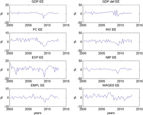
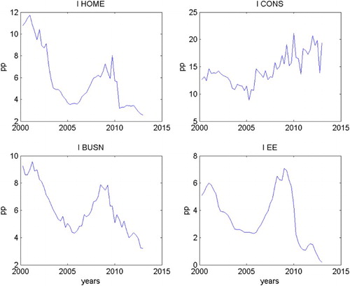
Figure 2 plots the Estonian three-month nominal money market interest rate (I), and loan interest rates by three loan types: the housing loan interest rate (I HOME); the consumer credit interest rate (I CONS); and the business loan interest rate (I BUSN). All interest rates except consumer credit have a downward trend that is linked to falling risk premium charged by the banks. A linear trend is added to all Estonian interest rates in the estimated models and the linear trend for the consumer credit interest rate series can pick up the increasing risk premium charged by the banks.

Figure 2. Estonian loan interest rates by type.

Note: All variables in levels.

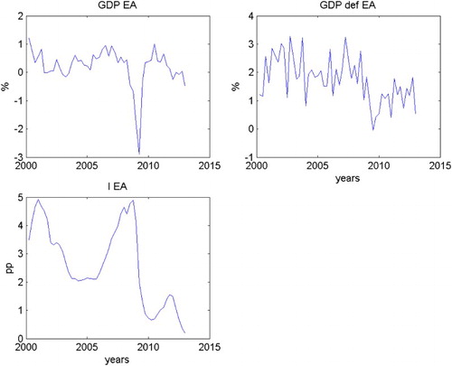
The three euro area time series used in the SVAR are presented in Figure 3. The overall dynamics of the euro area variables are similar to those of their Estonian counterparts. However, the mean and the variance of the Estonian GDP growth rate and the GDP deflator-based inflation rate are higher. From the theoretical point of view all series included in the models should be stationary. However precise time-series properties of the realization of the series have to be tested. Unfortunately given the short data period with a large shock and possible break in the sample, the tests do not have good properties and have to be treated with care. In order to get an idea of the time-series properties of our period, we tested for the unit root properties of the data with the Augmented Dickey Fuller test. The unit root of the euro area GDP, the euro area GDP deflator level, Estonian GDP, wages, employment, export, import levels, and the GDP deflator-based inflation rate could not be rejected at the conventional statistical levels. The unit root in these variables was rejected at first differences. The tests for stationarity of the Estonian investments and private consumption are of some concern. For the first difference the unit root can be rejected only at the 5% level. The unit root can be rejected safely at conventional levels only when the second difference of these series is used. However based on the theoretical considerations and the stationarity of the aggregate GDP series we proceed under the hypothesis that the first difference of the series is stationary. In addition the unit root of the Estonian and the euro area interest rate levels cannot be rejected. However the interest rates in theory should be stationary, so we use time trends and assume stationarity of the interest rates in the econometric analysis. Alternatively the regression model can be thought of as using an implicit cointegrating relationship. By looking at the chart (Figures 2 and 3), one can see that the Estonian and the euro area interest rates have a common pattern. Also Estonian macroeconomic variables are closely related, leading to implicit cointegrating relationships.

Figure 3. Euro area economic variables.

Note: GDP and GDP deflator in first differences, 3-month Euribor in levels.

The stylized facts about the business cycle for Estonian variables give background for understanding the relationship between the Estonian variables and Estonian and euro area GDP. Following Kydland and Prescott (1990), we use HP filtered data ( = 1600) on levels (differently from the SVAR). Table 1 shows the volatility of Estonian and euro area economic and financial data. The HP filter is known to be a robust method of separating cycles from the trend and discussing the stylized facts of the cycle. However, as the HP filter is two-sided and uses information from future periods which is not observable to the policy maker, it should not be used in the structural estimation of VAR models.

Table 1. Business cycle indicators.

Variable	St.dev.	Ratio to GDP^EE	Ratio to GDP^EA
GDP^EE	5.0	1.0	3.7
PC^EE	5.3	1.1	3.9
INV^EE	15.2	3.0	11.1
EXP^EE	8.9	1.8	6.6
IMP^EE	11.9	2.4	8.8
EMPL^EE	3.3	0.7	2.4
WAGES^EE	3.6	0.7	2.6
GDP def^EE	6.4	1.3	4.7
I HOME^EE	1.1	0.2	0.8
I CONS^EE	1.6	0.3	1.2
I BUSN^EE	0.8	0.2	0.6
I^EE	1.1	0.2	0.8
GDP^EA	1.4		1.0
PC^EA	0.5		0.4
INV^EA	3.4		2.5
EMPL^EA	0.6		0.5
WAGES^EA	0.2		0.2
GDP def^EA	0.7		0.5
I^EA	0.9		0.6

Notes: Calculated from data used in this paper for 2000Q1 to 2012Q4. GDP, real gross domestic product; PC, real private consumption; INV, real corporate investment; EXP, real exports; IMP, real imports; EMPL, employment; WAGES, real wages; GDP def, the GDP deflator-based inflation rate; I HOME, the housing loan interest rate; I CONS, the consumer credit interest rate; I BUSN, the business loan interest rate; I^EE, three-month Talibor; I^EA, three-month Euribor. Superscript EE stands for Estonia and EA for the euro area.

Estonian GDP is about 3.7 times more volatile than the GDP of the euro area. Although the most volatile component of Estonian GDP is corporate investment, like in the euro area, relative volatility to GDP is lower in Estonia. In contrast to the situation in the euro area, private consumption in Estonia is more volatile than GDP. Estonian imports are also very volatile, especially relative to exports. Relative to GDP, Estonian employment is as volatile as that in the euro area, but we observe remarkable differences in wages, with Estonia having a fairly high level of wage volatility. It is not unexpected for a small country to have a relatively high level of volatility in comparison to the aggregate euro area data, but the quantitative difference is high. There are also several differences in the relative importance of the components of GDP and the volatility of macro aggregates to GDP.

Table 2 presents the correlation of economic and financial indicators with Estonian real GDP^EE. It shows that to some extent GDP has forecasting power on many macroeconomic aggregates. However the GDP deflator-based inflation rate seems to have predicting power for GDP dynamics. Table 2 also shows that financial indicators have small contemporaneous correlation with GDP, but there is some evidence that interest rates lead the dynamics in GDP.

Table 2. Correlation of economic and financial indicators with Estonian real GDP.

Variable	Lags and leads
	xt−4	xt−3	xt−2	xt−1	xt	xt+1	xt+2	xt+3	xt+4
GDP^EE	0.33	0.58	0.77	0.92	1.0	0.92	0.77	0.58	0.33
PC^EE	0.23	0.48	0.69	0.85	0.95	0.95	0.86	0.72	0.53
INV^EE	0.24	0.46	0.67	0.82	0.91	0.90	0.82	0.66	0.46
EXP^EE	0.45	0.60	0.73	0.79	0.79	0.69	0.48	0.23	–0.01
IMP^EE	0.45	0.63	0.79	0.89	0.91	0.82	0.62	0.38	0.12
EMPL^EE	0.01	0.21	0.46	0.67	0.83	0.93	0.90	0.79	0.62
WAGES^EE	–0.18	0.05	0.21	0.36	0.50	0.56	0.59	0.61	0.59
GDP def^EE	0.30	0.33	0.34	0.39	0.25	0.33	0.14	–0.01	–0.06
I HOME^EE	–0.51	–0.43	–0.33	–0.22	–0.05	0.15	0.31	0.47	0.64
I CONS^EE	–0.18	–0.16	–0.14	–0.15	–0.06	–0.02	–0.10	0.12	0.10
I BUSN^EE	–0.64	–0.51	–0.35	–0.12	0.08	0.28	0.48	0.57	0.62
I^EE	–0.69	–0.57	–0.40	–0.19	0.05	0.33	0.57	0.75	0.85
GDP^EA	0.18	0.44	0.68	0.83	0.90	0.86	0.70	0.51	0.30

Notes: Lagging means correlation between GDP_t and PC_t−1 (forecasting power of PC on GDP); leading means correlation between GDP_t and PC_t+1 (forecasting power of GDP on PC). Data from 2000Q1 to 2012Q4. GDP, real gross domestic product; PC, real private consumption; INV, real corporate investment; EXP, real exports; IMP, real imports; EMPL, employment; WAGES, real wages; GDP def, the GDP deflator-based inflation rate; I HOME, the housing loan interest rate; I CONS, the consumer credit interest rate; I BUSN, the business loan interest rate; I^EE, three-month Talibor; I^EA, three-month Euribor. Superscript EE stands for Estonia and EA for the euro area.

4. Results

This section presents the main results. We visualize the effects of monetary policy shocks using impulse response functions (IRF). We accumulate the IRFs of the variables that are used in the SVAR in first differences (GDP, private consumption, corporate investment, exports, imports, employment, and real wages) with the exception of the GDP deflator-based inflation rate, which is shown as the inflation rate. The benchmark SVAR has two lags. All point estimates of IRFs are presented together with their centred 68% confidence intervals, calculated using the non-parametric bootstrap. The 68% intervals are approximately plus/minus one standard deviation. This allows the reader to visually depict plus/minus two or three standard deviations as well. The 68% confidence intervals are also popular in the recent SVAR literature.

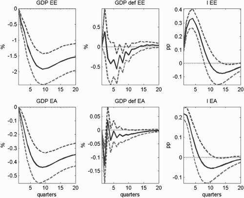
Figure 4 shows the reaction of Estonian and euro area GDP, GDP deflator-based inflation rates, and money market interest rates. A standard deviation increase in the Euribor of 22 bp dies out after five quarters. The Talibor increases on impact by 11 bp, reaches 34 bp by the fourth quarter, and converges back to zero by the eighth quarter.

Figure 4. Estimated impulse responses of Estonian and euro area GDP, the GDP deflator-based inflation rates, and the money market interest rates to a contractionary monetary policy shock in the euro area.

Note: The solid line describes point estimate and dashed lines 68% confidence intervals.

In the quarter after the shock, the Estonian GDP deflator-based inflation rate increases by about 0.4 pp, but subsequently falls to –0.6 pp. Inflation stays below zero for about three years. There is some evidence of the price puzzle, but it is statistically not significant. The price puzzle has been found for many countries (for example, see Christiano et al. (2005) for the USA and Mojon and Peersman (2003) for countries in the euro area). We find no evidence of the price puzzle for the euro area GDP deflator-based inflation rate, which falls one quarter after the shock by 0.1 pp, is then volatile, and converges back to zero after four years.

The effect of the shock on the GDP level is strong and persistent. Euro area GDP falls by about 0.4%, reaching its lowest point after two years. Estonian GDP drops by 1.8% and also reaches the bottom after two years. The reaction of Estonian GDP is more than four times stronger than that of euro area GDP.

These results are similar to the estimates of Jeenas (2010). In a different 7-dimensional SVAR he also finds that a 25 bp increase in the 3-month Euribor leads to a 1.5% decrease in Estonian GDP. However euro area GDP drops by more than in our model. The effects of the monetary policy shock in the euro area on Estonian and the euro area inflation are almost identical in his paper. Jeenas (2010) also finds some evidence of the price puzzle in Estonian inflation.

Our estimates for the euro area effects are about twice as strong as the findings of Weber, Gerke, and Worms (2011) who use the same identification scheme and the euro area data from 1996 to 2006. The difference is mainly due to the inclusion of data from the great recession. In the robustness analysis we show that our estimates are very close to their estimates when we use data from 2000 to 2007.

The monetary policy shock in the euro area also has strong effects on several other Estonian economic indicators. Figure 5 plots the IRFs estimated in separate SVAR models for private consumption, corporate investment, employment, real wages, imports, and exports. These Estonian variables give a broader picture of monetary policy transmission in Estonia. As Estonian variables do not affect euro area variables ( = 0), the IRFs for the euro area data are identical and therefore not reported.

Figure 5. Estimated impulse responses of additional Estonian macroeconomic variables to a contractionary monetary policy shock in the euro area.

Note: The solid line describes point estimate and dashed lines 68% confidence intervals.

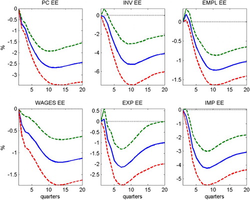
All variables follow a hump-shaped response. Private consumption drops by a maximum of 2.7% and corporate investment by 5.2%. Employment and real wages decrease to a lesser extent, falling by only 1.3% and 1.2% and reaching their lowest levels around 10 quarters after a monetary policy shock in the euro area. Exports decrease by around 2.2% by the eighth quarter and converge near the baseline after four years. Imports drop by 4.2% and stay low subsequently. The relatively small reaction of exports compared to the change in Estonian GDP leaves little room for the argument that foreign demand is the main driver of the strong reaction found in the economic aggregates. Instead the strong reaction of imports shows that there is a steep drop in domestic demand.

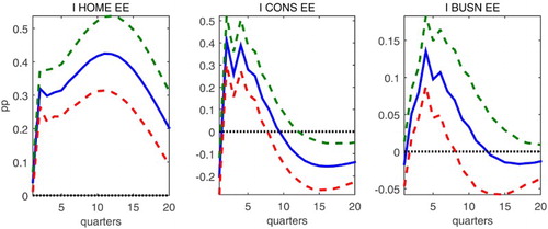
Figure 6 plots IRFs for the different Estonian loan interest rates. We use these three variables for two reasons. Firstly they are interesting as they show the money market interest rate pass-through to Estonian three loan type specific loan interest rates. Secondly they offer a possible explanation for the strong impact observed on the real economy.

Figure 6. Estimated impulse responses of loan type specific interest rates to a contractionary monetary policy shock in the euro area.

Note: The solid line describes point estimate and dashed lines 68% confidence intervals.

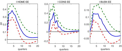
The housing loan interest rate rises on impact by about 12 bp and increases by up to 38 bp the year after, later converging slowly to zero. Strong contemporaneous pass-though is expected as a majority of housing loans have interest rates that are fixed to the six-month Euribor with an added risk premium. The pass-through to the housing loan interest rate is not direct as the dynamics of the six-month Euribor interest rate are somewhat different to those of the three-month Euribor and the risk premium charged on top of the Euribor is variable. The consumer credit interest rate has almost no contemporaneous pass-through, but reaches 40 bp after a year and converges back to the baseline after 10 quarters. The reaction of the business loan interest rate shows that there is no contemporaneous pass-through. The business loan interest rate increases by only 13 bp after 2 quarters.

Our results show that Estonian data are volatile at least partly because of internal amplification. By construction the identified shock is identical for the euro area and for Estonia, but the reaction of the Estonian variables is stronger. Our conjecture is that the interest rates have been at least partly responsible for the amplification of the euro area monetary policy shock in Estonia. In addition we find that housing loan and consumer credit interest rates react very strongly and sluggishly. An increase in the money market interest rate leads to a stronger increase in these interest rates.

The strong reaction of consumer credit and housing loan interest rates stands in contrast to the findings for the euro area of Giannone et al. (2012). They find that interest rates for consumer credit, housing, and corporate loans react substantially less than the money market interest rate. Similarly, the immediate pass-through of Estonian loan interest rates is also smaller than one. In contrast the Estonian money market, housing loan, and consumer credit interest rates react more than twice as strongly as the euro area money market interest rate. This indicates that the financial sector plays possibly an important transmission and amplification channel in monetary transmission. Our results indicate that the foreign demand channel could be of secondary importance as Estonian exports react by as much as GDP. In contrast, Estonian imports, which are affected by domestic demand, react about twice as strongly as Estonian GDP.

The residuals of the models have no unit root, confirming the hypothesis that possible non-stationarity issues can be resolved by implicit cointegration. We also tested for autocorrelation in the residuals and rejected that there is any remaining autocorrelation left. The Jarque-Bera test for normality executed in E-Views showed that normality can be rejected for some of the residual series. This is confirmed by eyeballing the histograms of the residuals. This gives additional motivation to analyse stability of the results over time and discuss the effect of the crisis and extreme observations.

5. Robustness analysis and the importance of the great recession

In this section we present the results for the stability and robustness analysis. We concentrate on the sensitivity to different lag lengths, the size of the SVAR, and possible effects of the length of the time series and of extreme observations in the sample. This sheds light on potential structural breaks without formally testing for them. Formal testing is prone to giving misleading results because of the low degrees of freedom and the possible structural break at the end of the sample.

The autoregressive model is known to be a good approximation of the underlying moving average process only when a sufficient number of lags are included. We also estimated models with three and four lags (results not shown). In the models with three and four lags the qualitative results remained the same, although the precision of the estimates deteriorated due to multicollinearity. The models with one lag SVAR were unstable and theoretically less interesting as they are not able to generate a hump-shaped response for the economic variables.

We also estimated a smaller model with six variables (Estonian and euro area GDPs, GDP deflator-based inflation rates, and money market interest rates). All other assumptions were the same as in the seven-dimensional SVAR. The results remained qualitatively unchanged. The only difference in the results was that the reaction of the Estonian variables was in some cases quantitatively somewhat smaller. Missing variable bias is likely to be small as the estimated IRFs for the main variables in the various models remain largely unchanged.

5.1. Sensitivity to extreme observations

Ordinary least squares estimations are known to be sensitive to outliers and extreme values in the data. The tests show that for some of the residual series of the benchmark model normality can be rejected. Residuals of the benchmark model have fat tails and are skewed. As the Estonian data do have high variance, especially during the recent crisis episode, we therefore remove some of the variance by including dummies as a robustness exercise. The use of dummies will give an indication of how much IRFs depend on the extreme observations. Dummies are used only in the Estonian data. We do not include dummies in the euro area equations because the main aim of the paper is to identify the euro area monetary policy transmission in Estonia. Moreover from the benchmark model we saw stronger reactions in the Estonian variables than in the euro area aggregates, motivating further the analysis of the Estonian data reaction separately from the euro area reactions. Ciccarelli, Maddaloni, and Peydró (2013) give a good overview of the possible changes of the monetary transmission mechanism in the euro area.

After estimating the model we identify potential extreme observations in the data by analysing the residual time series and histograms. After that we include dummies for the most extreme observations and then re-estimate the model and repeat the residual analysis and dummy introduction. The maximum number of dummies allowed by the equation was set at 12, but in some cases fewer dummies were used if the quantitative results remained unchanged or the impulse response functions became extremely volatile. Table 3 shows how many dummies are included in the final models. Outlier removal based on extreme residuals is a standard procedure and widely used in econometrics. Of course, the use of dummies comes at a price of losing valuable information of the data. In a small sample like ours, this might lead estimates to be biased towards zero, that is, underestimation of the true effect.

Table 3. Number of dummies in models.

Models with	GDP	Additional variable	GDP def	INV
PC	8	6	7	7
INV	8	3	5	3
EXP	12	8	7	7
IMP	11	8	10	6
EMPL	9	8	8	7
WAGES	6	9	9	6
I HOME	8	11	7	7
I CONS	8	12	7	7
I BUSN	8	8	7	7

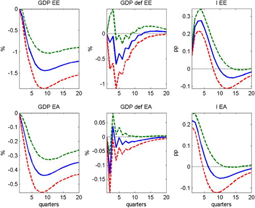
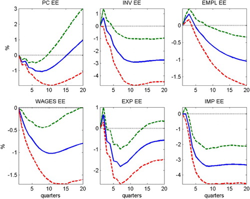
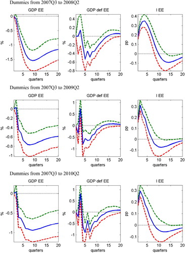
Figure 7 plots the results with the dummies included for the three main Estonian variables. The observed increase in GDP is somewhat lower, but still much stronger from the euro area counterpart. The GDP deflator-based inflation rate declines after the shock and does not show the price puzzle. The money market interest rate behaviour is largely unchanged, increasing by only a few basis points less than in the benchmark model.

Figure 7. Estimated impulse responses of Estonian and euro area GDPs, the GDP deflator-based inflation rates, and the money market interest rates to a contractionary monetary policy shock in the euro area. Dummies used in the Estonian data equations.

Note: The solid line describes point estimate and dashed lines 68% confidence intervals.

Figure 8 plots the results for private consumption, corporate investment, exports, imports, employment, and wages. The use of dummies reduces the impact of monetary policy shock the most in private consumption and corporate investment (see benchmark results, Figure 5).

Figure 8. Estimated impulse responses of additional Estonian macroeconomic variables to a contractionary monetary policy shock in the euro area. Dummies used in Estonian equations.

Note: The solid line describes point estimate and dashed lines 68% confidence intervals.

Figure 9 plots the results for the different loan interest rates. Dummies did not reduce the reactions (for comparison see benchmark results, Figure 6). On the contrary, all variables showed stronger movements after the shock.

Figure 9. Estimated impulse responses of loan type specific interest rates to a contractionary monetary policy shock in the euro area. Dummies used in Estonian equations.

Note: The solid line describes point estimate and dashed lines 68% confidence intervals.

We can also discuss the effects of the recent financial and economic crisis on monetary transmission. By looking at the Estonian time-series dynamics we use dummies for the period from 2007Q3 to 2010Q2. Dummies are used for three different sub-periods – 2007Q3 to 2008Q2, 2007Q3 to 2009Q2, and 2007Q3 to 2010Q2 – and named the one-year, two-year, and three-year models with dummies.

The three panels in Figure 10 plot the results with the dummies included for the three main Estonian variables. The money market interest rate dynamic is largely unchanged from the benchmark model, but the increase on impact is somewhat stronger at 19 bp. The GDP deflator-based inflation rate does not show the price puzzle, but the decline is stronger in all models with dummies than in the benchmark results. The reaction of GDP is smaller in the two-year and three-year models with dummies, hinting that the strongly amplified reaction in the benchmark model was partly caused by the strong impact measured during the crisis years.

Figure 10. Estimated impulse responses of Estonian GDP, the GDP deflator-based inflation rate, and the money market interest rate to a contractionary monetary policy shock in the euro area. Dummies used in the Estonian data equations for different time periods indicated for each panel separately.

Note: The solid line describes point estimate and dashed lines 68% confidence intervals.

The effects of the shock on additional Estonian economic and financial variables depend on the inclusion of crisis years in the data. The differences are bigger when dummies are used for the period from 2007Q3 to 2009Q2 and from 2007Q3 to 2010Q2 (results not presented). Estonian macroeconomic variables react less strongly, and for example the reaction is smaller in the one-year model with dummies for employment, which falls after the shock by 0.7%, and for real wages, which fall after the shock by 0.8%. In the two-year model with dummies the reaction is smaller for private consumption, which falls after the shock by 0.3%, and for imports, which fall after the shock by 1.2%. However, there are still signs of the price puzzle in the GDP deflator-based inflation rate.

The money market interest rate increases less, though interest rates for some loan type increase by more than in the benchmark model. The reaction of some variables (corporate investment, exports, and real wages) change signs when dummies are used for the period from 2007Q3 to 2009Q2 and from 2007Q2 to 2010Q2.

5.2. Stability of results over time

Giannone et al. (2012) find evidence that during the crisis period, from August 2007 to August 2010, the cyclical behaviour in some financial variables, such as longer term loans, deposits, and longer term interest rates, changed. Ciccarelli et al. (2013) also find that the crisis years have affected economic and financial developments in individual countries.

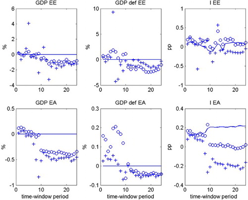
Testing for the changes in transmission with limited time series and a possible structural break in the later part of the sample is statistically complicated. However, in order to get some indication of possible changes, we use the simple approach of estimating the model in different rolling time-windows. The approach gives an intuitive understanding of possible changes in the euro area monetary policy transmission mechanism.

Table 4 shows how the whole period is divided into 24 rolling time-windows of 29 quarters (7 years and 1 quarter). The first period is from 2000Q1 to 2007Q1, the second is from 2000Q2 to 2007Q2, etc. We use 29 quarters of data as it allows us to estimate the first SVAR model in a period with no financial crisis reaching up to the second half of 2007. By adding quarters to the end and subtracting from the beginning, the financial crisis and the subsequent sovereign debt crisis are covered. Shortening the period further becomes difficult as the degrees of freedom drop drastically.

Table 4. Time-windows.

Time-window	Beginning		End
1	2000	Q1	2007	Q1
2		Q2		Q2
3		Q3		Q3
4		Q4		Q4
5	2001	Q1	2008	Q1
6		Q2		Q2
7		Q3		Q3
8		Q4		Q4
9	2002	Q1	2009	Q1
10		Q2		Q2
11		Q3		Q3
12		Q4		Q4
13	2003	Q1	2010	Q1
14		Q2		Q2
15		Q3		Q3
16		Q4		Q4
17	2004	Q1	2011	Q1
18		Q2		Q2
19		Q3		Q3
20		Q4		Q4
21	2005	Q1	2012	Q1
22		Q2		Q2
23		Q3		Q3
24		Q4		Q4

Estimation of the models for the early period showed no (or even reverse) effects of monetary policy in either the euro area or Estonia. If we look at the periods until 2009, a contractionary monetary policy shock leads to a small but persistent increase in the GDP deflator-based inflation rate and the GDP level in both the euro area and Estonia (see Figure 11). The euro area result is similar to the result of Weber et al. (2011) for the period 1999–2006. The Estonian results are in line with the anecdotal evidence that probably monetary policy shocks in the euro area did not play an important role in the Estonian economy until the economic slowdown. Contrary to standard intuition Männasoo (2007) even found that during the years between 1994 and 2004 the number of firms failing in Estonia decreases after an interest rate hike.

Figure 11. Selected points in impulse responses of Estonian and euro area GDP, the GDP deflator-based inflation rates, and the money market interest rate to a contractionary monetary policy shock in the euro area using rolling time-windows.

Note: The solid line (—) describes the immediate IRF to the variable of each time-window. The circle (○) describes the IRF after four quarters (one year) of each time-window. The cross (++) describes the IRF after eight quarters (two years) of each time-window.

For the period before the crisis years we also get opposite reactions from those of the benchmark results for other Estonian macroeconomic variables (see Figures 12 and 13). The dynamics of exports, imports, real wages, corporate investment, and private consumption follow the behaviour of Estonian GDP. The results for exports and real wages are somewhat stronger in the models with time-windows, meaning the impact of the beginning of the 2000s is important for the benchmark model.

Figure 12. Selected points in impulse responses of additional Estonian macroeconomic variables to a contractionary monetary policy shock in the euro area using rolling time-windows.

Note: The solid line (—) describes the immediate IRF to the variable of each time-window. The circle (○) describes the IRF after four quarters (one year) of each time-window. The cross (+) describes the IRF after eight quarters (two years) of each time-window.

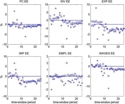
Figure 13. Selected points in impulse responses of Estonian loan type specific interest rates to a contractionary monetary policy shock in the euro area using rolling time-windows.

Note: The solid line (—) describes the immediate IRF to the variable of each time-window. The circle (○) describes the IRF after four quarters (one year) of each time-window. The cross (+) describes the IRF after eight quarters (two years) of each time-window.

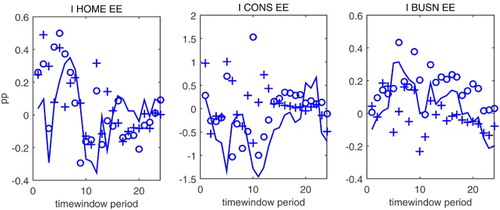
The estimated effects look very close to our benchmark results when the data from the last quarters of 2008 and first quarters of 2009 are included in the sample. Some of the models for data periods ending in the middle of the crisis are hard to estimate and the SVAR models become unstable. But then the results stabilize and stay close to our benchmark results for the later samples, although the magnitude might be a little muted. This holds again both for the euro area and for Estonia.

5.3. Private loan quantities

Strong reaction of the interest rates motivates further analysis of the financial sector behaviour. Moreover Estonia faced a remarkable credit boom–bust cycle during the period of study. In order to control for the credit boom, we re-estimate the model including three loan quantities. Following the division of the loans for the interest rates, we include the real business loans, mortgages, and consumption credit growth rates in the model. The data come from the Bank of Estonia public statistical database. The results show strong reaction of loan quantities to the monetary shock. The growth rate of loans is on average four times stronger than the effect on the GDP level, leading to substantial change in the credit to GDP ratio five years after the shock. The results on the effects of the shock on credit measures has to be taken with great care as loan time series are not well behaved. The period starts with strong credit growth which flattens out in the second part of the sample. Extraction of the credit deepening episode from the credit boom–bust cycle is a controversial exercise. However we find that other variables in the system react similarly to the benchmark model, confirming benchmark results and showing that the missing variable bias from the exclusion of the credit measures is most likely small.

6. Conclusion

In this paper we estimate the transmission of the monetary policy shocks in the euro area to Estonian economic and financial variables. We find that a 22 basis points increase in the euro area money market interest rate increases the Estonian money market interest rate by a maximum of 34 basis points and leads to a substantial increase in the housing loan and consumer credit interest rates. The shock brings down Estonian GDP by almost 1.9% and the GDP deflator-based inflation rate by 0.6 percentage points. We conclude that the trade channel is less likely to be responsible for the large effects observed in the macroeconomic aggregates. Exports decrease by substantially less than imports, private consumption, or GDP. We conjecture that the strong reaction of GDP and its components can be partly assigned to a large increase in housing loan and consumer credit interest rates.

Acknowledgements

The views expressed are those of the authors and do not necessarily represent the official views of Eesti Pank. We would like to thank the Editor, two anonymous referees, Rasmus Kattai, Merike Kukk, Dmitry Kulikov, Martti Randveer, Karsten Staehr, and all the participants of the seminars at the Bank of Estonia, ECEE conference in Tallinn, the Baltic Central Bank meeting in Riga, and the NBP workshop Monetary transmission mechanism in diverse economies in Warsaw for their helpful comments.

Disclosure statement

No potential conflict of interest was reported by the author(s).

Notes

1. However, our results cannot fully exclude the possibility that the risk premium component in loan type specific interest rates reacts to the substantial and persistent drop in GDP. If this were true, then the interest rate on business loans could move similarly.

2. The Bank of Estonia stopped collecting Estonian money market interest rate data from January 2011 as Estonia joined the euro area. We use Talibor until 2010Q4 and the three-month Euribor thereafter.

Appendix

Data sources

Table A1. Data sources for Estonia from 2000Q1 to 2012Q4.

Variable	Transf.	Source
GDP	log diff.	Eurostat: GDP and main components – volumes [namq_gdp_k] (gross domestic product at market prices, chain linked volumes, 2005=100, seasonally adjusted and adjusted data by working days)
GDP deflator	log diff.	Eurostat: GDP and main components – volumes [namq_gdp_k] and GDP and main components – Current prices [namq_gdp_c] (gross domestic product at market prices, chain linked volumes, 2005=100, seasonally adjusted and adjusted data by working days)
3-month Talibor	level	Eurostat: 3-month rates for Estonia, quarterly data [irt_h_mr3_q]
Private consumption	log diff.	Eurostat: GDP and main components – volumes [namq_gdp_k] (final consumption expenditure of NPISH, chain linked volumes, 2005=100, seasonally adjusted and adjusted data by working days)
Corporate investment	log diff.	Eurostat: GDP and main components – volumes [namq_gdp_k] (gross fixed capital formation, chain linked volumes, 2005=100, seasonally adjusted and adjusted data by working days)
Exports	log diff.	Eurostat: GDP and main components – volumes [namq_gdp_k] (exports of goods and services, chain linked volumes, 2005=100, seasonally adjusted and adjusted data by working days)
Imports	log diff.	Eurostat: GDP and main components – volumes [namq_gdp_k] (imports of goods and services, chain linked volumes, 2005=100, seasonally adjusted and adjusted data by working days)
Wages	log diff.	ECB: Estonia – Compensation Per Employee, current prices, national currency, working day and seasonally adjusted, Index [ESA.Q.EE.Y.1000.COMEMP.0000.TTTT.V.N.I]; deflated by the consumer price index
Employment	log diff.	Eurostat: Population and employment – quarterly data [namq_aux_pem] (total employment, domestic concept, 1000 persons, seasonally adjusted and adjusted data by working days)
The housing loan interest rate	level	Eesti Pank: Table 3.7.3 Interest rates of loans granted to households by loan type and currency
The consumer credit interest rate	level	Eesti Pank: Table 3.7.3 Interest rates of loans granted to households by loan type and currency
The business loan interest rate	level	Eesti Pank: Table 3.7.2 Interest rates of loans granted to non-financial corporations by borrower's main economic activity

Table A2. Data sources for the euro area from 2000Q1 to 2012Q4.

Variable	Transf.	Source
GDP	log diff.	Eurostat: GDP and main components – volumes [namq_gdp_k] (gross domestic product at market prices, chain linked volumes, 2005=100, seasonally adjusted and adjusted data by working days)
GDP deflator	log diff.	Eurostat: GDP and main components – volumes [namq_gdp_k] and GDP and main components – Current prices [namq_gdp_c] (gross domestic product at market prices, chain linked volumes, 2005=100, seasonally adjusted and adjusted data by working days)
3-month Euribor	level	ECB: Money market rates/Euribor three-month funds/Monthly average [SU0316]

References

- Angeloni, I., Kashyap, A., Mojon, B., & Terlizzese, D. (2003). Monetary policy transmission in the euro area: Where do we stand? In Angeloni, I., Kashyap, A., and Mojon, B. (Eds.), Monetary policy transmission in the Euro area (pp. 383–412). Cambridge University Press, 2003, chapter 24.
- Bernanke, B. S., & Gertler, M. (1995). Inside the black box: The credit channel of monetary policy transmission. Journal of Economic Perspectives, 9(4), 27–48. doi: 10.1257/jep.9.4.27
- Christiano, L. J., Eichenbaum, M., & Evans, C. L. (1996). The effects of monetary policy shocks: Evidence from the flow of funds. The Review of Economics and Statistics, 78(1), 16–34. doi: 10.2307/2109845
- Christiano, L. J., Eichenbaum, M., & Evans, C. L. (1999). Monetary policy shocks: What we have learned and to what end? Handbook of Macroeconomics, 1A, 65–148. doi: 10.1016/S1574-0048(99)01005-8
- Christiano, L. J., Eichenbaum, M., & Evans, C. L. (2005). Nominal rigidities and the dynamic effects of a shock to monetary policy. Journal of Political Economy, 113(1), 1–45. doi: 10.1086/426038
- Ciccarelli, M., Maddaloni, A., & Peydró, J.-L. (2013). Heterogeneous transmission mechanism: Monetary policy and financial fragility in the eurozone. Economic Policy, 28(75), 459–512. doi: 10.1111/1468-0327.12015
- Corsetti, G., Dedola, L., & Leduc, S. (2014). The international dimension of productivity and demand shocks in the US economy. Journal of the European Economic Association, 12(1), 153–176. doi: 10.1111/jeea.12070
- Elbourne, A., & de Haan, J. (2009). Modeling monetary policy transmission in acceding countries: Vector autoregression versus structural vector autoregression. Emerging Markets Finance and Trade, 45(2), 4–20. doi: 10.2753/REE1540-496X450201
- Errit, G., & Uusküla, L. (2013). Euro area monetary policy transmission in Estonia. Bank of Estonia Working Papers, no. 7.
- Giannone, D., Lenza, M., & Reichlin, L. (2012). Money, credit, monetary policy and the business cycle in the euro area. CEPR Discussion Papers no. 8944.
- Jacobs, J., Kuper, G. H., & Sterken, E. A. (2003). Structural VAR model of the euro area. mimeo.
- Jeenas, P. (2010). Analysis of Estonian aggregate data using VAR models. Eesti Pank, mimeo.
- Kydland, F. E., & Prescott, E. C. (1990). Business cycles: Real facts and a monetary myth. The Federal Reserve Bank of Minneapolis quarterly review, 1421, 3–18.
- Lättemäe, R. (2003). Monetary transmission mechanism in Estonia. Kroon and Economy, (1), 58–67.
- Männasoo, K. (2007). Determinants of firm survival in Estonia. Bank of Estonia Working Paper no. 4.
- Mojon, B., & Peersman, G. (2003). A VAR description of the effects of monetary policy in the individual countries of the euro area. In Angeloni, I., Kashyap, A., and Mojon, B. (Eds.), Monetary policy transmission in the Euro area (pp. 56–74). Cambridge University Press, 2003, chapter 3.
- Peersman, G., & Smets, F. (2003). The monetary transmission mechanism in the euro area: More evidence from VAR analysis. In Angeloni, I., Kashyap, A., and Mojon, B. (Eds.), Monetary policy transmission in the Euro area (pp. 36–55). Cambridge University Press, 2003, chapter 2.
- Soares, R. (2011). Assessing monetary policy in the euro area: A factor-augmented VAR approach. Bank of Portugal Working Paper no. 11.
- Weber, A. A., Gerke, R., & Worms, A. (2011). Changes in euro area monetary transmission? Applied Financial Economics, 21(3), 131–145. doi: 10.1080/09603107.2010.526580