The contribution of R&D to production efficiency in OECD countries: econometric analysis of industry-level panel data

Abstract

While research and development expenditures are considered a key to productivity growth and development, the question remains whether their contribution could depend on the particular countries’ and industries’ actual development levels and positions in global value chains. In this paper we analyse the relative contribution of R&D to the efficiency (productivity) on the industry and sector level in OECD countries using industry-level panel data and the stochastic frontier production function approach. The results indicate that R&D capital productivity enhancing effect increases with the level of technology; physical capital shows the opposite effect. The distribution of efficiency across industries shows remarkably different variances, reflecting different degrees of competition and the structure of value chains. Among different external factors, the share of labour with tertiary education at the national level showed a strong positive correlation with efficiency, while for other external factors the effect varied across the industries. The findings imply that in the design of R&D policy measures the structure of the industries needs to be considered.

Keywords:

• efficiency
• R&D
• SFA
• technological change

JEL classification codes:

• O32
• O39

1. Introduction

Innovation is increasingly acknowledged as the key to productivity growth and development, both in developed countries but increasingly also for the developing and catching up economies (Fagerberg, Srholec, & Verspagen, 2010). That has been understood by policymakers around the world and reflected in different countries setting targets for innovation inputs and outputs, probably the most well-known one being the Lisbon target, setting the R&D expenditures to the 3% level of GDP.¹ It has also been questioned whether the same targets should be set for countries at different levels of development and different industrial structures (dominating low-tech or high-tech industries) and whether the indicators used to compare countries’ innovation performance, like the European Innovation Scoreboard, are always meaningful (e.g. Schibany & Streicher, 2008). While at the micro level the positive relationship between innovation and productivity is mostly revealed (Mairesse & Mohnen, 2010), the R&D is not equally important in different sectors (Kumbhakar, Ortega-Argilés, Potters, Vivarelli, & Voigt, 2012), the relationship between R&D expenditures and GDP growth does not always show up (Pessoa, 2010), there could be some necessary minimal critical level for the positive relationship to show up (Kancs & Siliverstovs, 2012). That motivates the study of the comparison of the efficiency of the innovation production processes in different countries.

The aim of the article is to analyse the contribution of research and development to the efficiency (productivity) of enterprises at industries with various technological levels in Organization for Economic Co-operation and Development (OECD) countries. For the analysis we use the stochastic frontier production function approach (which goes back to Aigner, Lovell, & Schmidt, 1977); for an overview of SFA (stochastic frontier analysis) approaches see e.g. Coelli, Rao, O'Donnell, and Battese (2005) in order to account for how the total factor productivity and production efficiency are influenced by various factors of production (labour, physical capital, R&D capital) on the one hand, and the various environmental factors (factors external to the enterprises), like the societies technological level and quality of the human capital, on the other hand. The industry-level data are from OECD STAN (indicators of labour, capital, etc.) and ANBERD  (R&D expenditures) databases for 25 OECD countries for the period of 1987–2009. The variables for various external factors are extracted from the World Development Indicators database. For formulation of the policy goals in R&D one needs to consider the industrial specialization of the economy and the relative position of different industries in sectors of various technological levels. For instance, Kumbhakar et al. (2012) showed using data on the biggest European R&D performers that R&D was linked with higher productivity primarily in high-technology industries and not so in low-technology industries. Even the group of OECD countries is heterogeneous enough in terms of economic development and industrial structure,² therefore one common target for R&D expenditures in different countries need not be the optimal one. In addition, it has been shown by Pavitt (1984) that the technological development of different sectors does not necessarily rely on R&D but rather on learning by doing or learning by using processes. We acknowledge that the industry-level analysis has certain limitations, e.g. the R&D expenditures may differ across local and multinational firms (Johansson, Lööf, & Ebersberger, 2008) and it neglects how the R&D expenditure growth is divided between the growing expenditures in existing R&D performers and those starting R&D activities (Higon, Manez, & Sanchis-Llopis, 2011).

The analysis is motivated by the current focus of the R&D policies of the Baltic states. The R&D strategies have set quite ambitious targets for the level of R&D expenditures. For instance, in Estonia the strategy to raise the competitiveness of Estonia (‘Konkurentsivõime kava’, 2011) has set the target for R&D expenditures for 2020 at the level of 3% of GDP (the initial level in 2009 was 1.42%). In the case of Latvia, the Latvian National Development Plan for 2007–2013 set the target for 3% for 2013; the initial level was rather modest at 0.45% in 2009. The strategy for the later period, National Reform Programme of Latvia for the Implementation of the ‘Europe 2020’ strategy, set the target at 1.5% by 2020 (Masso, Liik, & Ukrainski, 2013). The case of Lithuania foresees the growth of R&D expenditures from 0.92% in 2012 to the level of 1.9% by 2020 (‘Lithuania: National Reform Programme’, 2013). The largest part of that growth should come from the business sector.³ Therefore, the relevant question is how much R&D could contribute to the growth of the Baltic states given the current economic conditions like the industrial structure of the economy. Though we did not have available the industry-level R&D expenditures data for Latvia and Lithuania, we think that our conclusions bear importance for all the Baltic countries given that despite differences the Baltics still form a relatively homogenous region.

In our analysis we essentially look at the input–output linkages and economic performance. While the innovation process has been regarded as a very complex one, its simplified linear version has still proved to be useful for empirical analysis. Griliches (1979) was the first to introduce the concept of knowledge production function, by which the combination of innovation inputs brings innovation outputs. This idea has been used later at firm-, industry- and country-level studies; Rousseau and Rousseau (1997) were the first to use the production frontier measurement approach to evaluate the cross-country innovation production performance. Several studies have followed from that (e.g. Wang, 2007; Zhang, Zhang, & Zhao, 2003). The studies have used different methods, either data envelope analysis (DEA) or stochastic frontier analysis. While most studies have estimated the simple relationship between inputs and outputs, Guan and Chen (2010) based their study on a model, where the innovation production process was divided into the R&D sub-process (relationship between innovation inputs and outputs) and commercialization sub-process (the relationship between outputs and outcomes, like innovation sales and productivity). From the literature on firm-level innovation performance, the Crépon, Duguet, and Mairesse (CDM, 1998) model estimated on the firm-level data of innovation surveys follows a similar logic (Mairesse & Mohnen, 2010): it models how innovation inputs (like R&D or innovation expenditures) are transformed into innovation outputs (patents, product, and process innovation, and sales of new products). Such a scheme has been generally proposed as suitable for the analysis of the efficiency of public spending (Mandl, Dierx, & Ilzkovitz, 2008).

There have been various studies on the analysis of the efficiency of innovation processes, research and development, and more broadly, national innovation systems using different econometric approaches and different kinds of data. According to Chaminade and Edquist (2010), the efficient functioning of a national innovation system (hereinafter NIS) assumes the provision of knowledge inputs to innovation process (provision of R&D, creation of new knowledge, competence building for innovations through education, etc.), encouragement of the demand-side of innovations (formation of markets for new products and articulation of quality requirements), provision of constituents of innovation systems (creating and changing organizations and institutions, but also networking), and provision of support services for innovating firms (incubation, financing, consultancy services). While the role of the government in NIS could be seen more broadly in favouring the self-organization of NIS (Edquist, Malerba, Metcalfe, Montobbio, & Steinmueller, 2004), in studies more narrowly focused on the function of government, it has been more common to focus on the direct investment on knowledge production and its relation with R&D investments by private firms. David, Hall, and Toole (2000) review the studies analysing the efficiency of R&D expenditure over 1965–2000 and find that generally, macro- and meso-level studies find complementarities between public and private R&D expenditure.

In most articles, the immediate outputs of different investments are considered shown by number of patents, publications, etc., while fewer studies consider outcomes of NIS in a broader sense and longer horizon. As one example, Guellec and van Pottelsberghe (2003) analysing 17 OECD countries over 1981–1996 (using a first-difference auto-regressive model) argued that any kind of government support when it is consistent, but also moderate in size (due to an inverted-U relationship) can be more effective in the long term as it reduces uncertainty for firms. The efficiency of R&D investments made by government depends on the functioning of the NIS determined by the appropriate alignment of the organizations in the system for smoother interactions within the NIS, but also on the favourable factors of the environment. Cincera, Czarnitzki, and Thorwarth (2009) assess the relationship between public R&D spending (inputs) inducing the additional R&D in the business sector, which is induced by public measures (output). The effects of R&D are then connected to different outcomes of these processes (output and TFP growth). For an overview of stochastic frontier analysis (hereinafter SFA) approaches see see e.g. Coelli, Rao, O'Donnell, and Battese (2005) in order to account for how the total factor productivity (hereinafter TFP) and production efficiency are influenced by various factors of production (labour, physical capital, R&D capital) on the one hand, and the various environmental factors (factors external to the enterprises), like the societies technological level and quality of the human capital, on the other hand. The resulting efficiency scores are then explained by different framework conditions of the NIS. Although they report variable results for different model specifications, they find that the framework conditions (access to sound money, and the legal structure and security of property rights) are improving the efficiency of public R&D investments.

Wang and Huang (2007) find that the national ratio of higher education as well as proficiency of English help to achieve higher efficiency of R&D investments. Somewhat similar results are found by Jaumotte and Pain (2005), showing that the availability of scientists and engineers, research conducted in the public sector, industry–academia knowledge exchange, the degree of product market competition, a high level of financial development, and access to foreign inventions would increase the R&D activities. In addition, the effect of direct public financial support for business R&D is generally positive (although modest), but intellectual property rights increase patenting while having little impact on R&D spending. Similarly, Falk and Leo (2006) find that although public R&D funding has positive effects, the dynamics of GDP growth and R&D prone industry structure (measured by the share in value added) seem to be more important drivers behind the business sector's R&D efficiency. By considering the efficiency of different specialized sub-processes (capital, labour technological balance of payment, article-oriented and patenting) in the NIS, Lee and Park (2005) have found that most Eastern European countries show low output efficiency in most sub-processes, with only Hungary showing a high efficiency in production of academic papers.

Given the previous literature, we can say that our analysis sheds additional light onto the importance of R&D on various industries and countries. The analysis contributes to the literature by investigating the ideas of Kumbhakar et al. (2012) with industry-level data on a wider set of countries. We also contribute by investigating how the linkage between production efficiency and R&D is influenced by various environmental factors like the use of ICT. In many countries the R&D policy documents specify ICT as one of the priority areas (Ukrainski, Kanep, & Masso, 2013), therefore it is important to investigate its role in the efficiency of R&D.

The rest of the article is structured as follows. The next section introduces the applied econometric approach, a stochastic frontier analysis based on the estimation of the production function. The third section describes the data and the model. The fourth section discusses the results and adds some more general policy implications. The final section concludes.

2. The method

Our analysis of the relationship between innovation inputs and output is based on the production function and SFA method. Using this method, we examine the extent to which the innovation input (R&D capital) influences the productivity of the industry, as well as its contribution relative to the other inputs. The existence of a common production possibility frontier for examined firms/industries/countries forms a base for SFA. If such a frontier exists, then it forms a best practice (efficiency frontier) relative to the sample producers. Whereas such an efficiency frontier is common to the whole sample, such relative productivity is called efficiency, and is measured as a percentage. The difference from a standard production function approach is that the production function is not an average over sample, but an extreme, which may be not achievable by the firms in the sample. In short, any firm in a particular sample is compared with the best practice, constructed on the basis of these same firms. All the comparison of the firms is based on the productivity.

Founders of SFA are Aigner et al. (1977) and Meeusen and van den Broeck (1977). Their approach is based on the idea that a firm's real output may be lower than that the production function enables. The reasons, for example, may be a random shock (e.g. bad weather in agriculture), or weak management. Such an idea is expressed in composite error terms, included into the production function, and consists of random noise and asymmetric inefficiency. A single-input production function with random noise and asymmetric inefficiency is as follows (Coelli et al., 2005): (1) where is a random noise and is a technical inefficiency. Inefficiency shows the deviation, by which the actual production differs from the ideal. In the case of , the result is a deterministic frontier; in the case of , the result is a stochastic frontier. There are four possible probability distributions of asymmetric error term: (1) exponential (Meeusen & van der Broeck, 1977); (2) half-normal (Aigner et al., 1977); (3) truncated normal (Stevenson, 1980); (4) Gamma (Greene, 1990). Transforming the logarithmic form of production function (1) to the exponential, technical efficiency could be expressed as a ratio of actual to the best practice production: (2) The main purpose of SFA models is to estimate the inefficiency term and corresponding efficiency (Greene, 2008, p. 114). The SFA model includes both the random noise and inefficiency; therefore, specific assumptions about independence of error terms and probability distribution of asymmetric error are necessary. In this case, the inefficiency term could be calculated, using Jondrow, Lovell, Materov, and Schmidt's (1982) approach (known as JLMS), based on conditional expectation . Jondrow et al. gave a solution for half-normal and exponential distribution. The conditional expectation of in the case of half-normal distribution is as follows: (3) where and are respectively standardized density and cumulative distribution function, composite error , parameters , . Truncated normal distribution is a general form of half-normal; therefore, conditional expectation of asymmetric error term is as follows (Greene, 2008, p. 177): (4) where is a mean value of . The aforementioned four inefficiency distributions give very close efficiency estimates (Greene, 2008, p. 182), exponential and truncated normal are almost identical. Different forms of inefficiency distributions do not significantly affect efficiency rankings and the composition of the upper and lower deciles (Greene, 1990). Gamma distribution is more complicated, different iterative methods must be used for estimation, therefore it is rarely used. In practical applications the half-normal is a typical choice (Kumbhakar & Lovell, 2000).

These relationships (Equations 1–4) are for cross-sectional models, which have several drawbacks. One of the biggest drawbacks is inconsistency of JLMS estimates, since the variance of does not converge to zero, as the size of the cross-section increases (Schmidt & Sickles, 1984). Adding more observations to each producer can increase the consistency of estimates, also strong distributional assumptions of error components could be mitigated (Kumbhakar & Lovell, 2000). Repeated observations for each producer help model time-varying inefficiency, but this is accompanied by two opposing arguments. A longer panel in the case of time-invariant inefficiency gives better consistency, but time-invariant inefficiency is less likely in the case of a longer panel. There is no simple solution to such a dilemma (Greene, 2008, p. 168).

In order to use the SFA method, the production function must be selected, for the best practice frontier. Two forms of functions are dominating in empirical applications (Greene, 2008, p. 98): Cobb-Douglas (CD) and translogarithmic. These functions are related, CD is a constrained version of translogarithmic function. With respect to efficiency estimates, there is no significant difference between these two, also the ranking of efficiency scores is strongly correlated (Zhang, 2012).

The SFA model selection is generally similar to panel data models – among the options are fixed and random effect models. The difference between these two is related to the assumptions about the asymmetric error term. The fixed-effect model does not need any assumptions about probability distribution of asymmetric error, which may be correlated with regressors or random noise, becoming a part of the producer-specific intercept parameter (Kumbhakar & Lovell, 2000). The fixed-effects model also has the advantage of simplicity and consistency of estimates, while it also has several drawbacks: inefficiency captures all time-invariant between-groups effects. Therefore, in fixed-effect models all time-invariant heterogeneity is included into inefficiency. Such an approach may be not consistent with reality and leads to overestimation of inefficiency (some effects do not belong to inefficiency). Another drawback is a substantially larger number of parameters to be estimated. The fixed-effect model fits better for estimating within-group effects, which could not be caused by heterogeneity (Kohler & Kreuter, 2005). The random effect model does not treat the inefficiency as a fixed, but as a random variable, which is not correlated with the explanatory variables (Greene, 2007). The random effect model is more appropriate if between-groups effects affect the dependent variable. A widely used Hausman specification test between the fixed and random effect is not appropriate, if there is heteroscedasticity or serial correlation (Baltagi, 2001). In such a case a better way to test it is by expanded regression (Wooldridge, 2010): (5) where is the dependent variable, are all explanatory variables and intercept; are time averages of all time-varying explanatory variables; has zero mean and is not correlated with . The null hypothesis for random effect is . Rejecting the null hypothesis means fixed-effect appropriateness. Robust errors could be used in this expanded regression. If estimates of the econometric model have no constant variance, then heteroscedasticity is present (Greene, 2007). SFA models are even more vulnerable than linear regression models, because there are two affected error components (Kumbhakar & Lovell, 2000). For such a case, robust White (1980) estimates could be used for standard errors. White's estimate is appropriate also in cases when the structure of heteroscedasticity is not known (Greene, 2007).

3. The data and the model

The study is based on industry-level (by International Standard Industrial Classification of All Economic Activities (ISIC) Rev. 3 two-digit industries) data from 25 OECD countries,⁴ over a 23-year period from 1987 to 2009, forming an unbalanced panel. Two OECD datasets were combined, OECD STAN (for measures of output, labour input, and capital) and OECD ANBERD (for research and development expenditures). Although the use of Eurostat data would seem to be more logical given our attention also on the R&D policies of the Baltic countries, we have used the OECD data for several reasons. OECD data include most of the EU countries. For Latvia the industry-level R&D data are anyway not available. The study of high-tech industry is not feasible without data from countries like the USA, Japan, and South-Korea. Differently, in order to construct the efficiency frontier we would need data from countries with the highest levels of productivity in the respective industries. In addition, for the study of the global value chains one cannot limit the attention to only the EU countries.

The following variables from these datasets were used hereinafter in order to calculate the model's input and output variables:

• EMPE – Number of employees;

• GFCF – Gross fixed capital formation at current prices;

• VALU – Value added at current prices;

• rdnat – R&D expenses (at current prices).

The aforementioned basic industry-level input and output variables are transformed for subsequent use. R&D expenditures and investments into physical capital must be capitalized, in order to provide R&D and physical capital stock variables.⁵ For this purpose the widely used perpetual inventory method (Hall, Mairesse, & Mohnen, 2010) is used. R&D capital stock in time period derives as follows: (6) where is the depreciation rate and means R&D expenses at period t. In addition, a starting value of R&D capital is calculated at the time period as follows: (7) where g is the growth rate of R&D expenses and is the depreciation rate, which together form the R&D capital discount rate. The latter relationship (5) means perpetuity value at the time t ₀, where period t ₀ is a first period of a panel. Growth rates are calculated according to data, depreciation rates are chosen depending on the industry's technology level (high, medium, and low-tech).⁶ The OECD classification enables grouping industries into four levels, based on the intensity of R&D expenditures⁷ (OECD, 2011): high-tech, low-tech, and medium-tech, which is divided into medium-high and medium-low. However, such a separation is made partially at three-digit level, which is not supported by our data. Therefore, we do not divide medium-tech any further. We use the following depreciation rates for R&D capital (the same as used by Kumbhakar et al., 2012): high-tech – 20%; medium-tech – 15%; low-tech – 12%. The depreciation rates for physical capital were respectively 8%, 6%, and 4%. Differences between depreciation rates across sectors are based on the idea that technologically more advanced products (e.g. cell phone versus bucket) and relevant technologies have on average shorter life-cycles.

The aforementioned technological levels are originally meant for the manufacturing industries, in this case the rest of the industries are classified as medium-tech. The service sector could in turn be divided into sub-sectors (Eurostat, 2014),⁸ but the data sample we used is too aggregated for such separation. Therefore, we do not distinguish between the services in detail. Inputs and output are transformed as ratios to the number of employees. As a result, the output variable is value added per unit of labour, i.e. labour productivity. Similarly, physical and R&D capital are also measured as per unit of labour basis (see Table 1).

Table 1. Descriptive statistics of external and production factors.

Variable	Description	No. of obs.	Mean	Std. Dev.	Min	Max
hedpart^a	Labour force with tertiary education (% of total)	6415	23.9	10.65	8.2	61.1
ictgoodsexp^a	ICT goods exports (% of total goods exports)	4159	9.1	8.09	0.07	36.8
ictgoodsimp^a	ICT goods imports (% total goods imports)	4159	10.8	5.58	3.52	35.9
intusers100^a	Internet users (per 100 people)	6394	34.2	25.87	0.07	90.8
mobilecell100^a	Mobile cellular subscriptions (per 100 people)	6415	62.9	41.22	0.10	151.2
Y	Y = VALU/EMPE	6415	77324	116587	1740.8	2826712
K	K = physical capital/EMPE	6415	186528	380489	236	8680612
R&D	R&D = R&D capital/EMPE	6415	14649	42210	0.06	1037032

Note: ^aThe World Bank, World Development Indicators.

Source: authors’ calculations. All national currencies are deflated and converted to euros.

Besides the transfer of the technology, a country's productivity growth also depends on diffusion⁹ and absorption of technology (Blomström, Lipsey, & Zejan, 1994). Here is the important role of the company's external environment (Teece, 2010). The absorption capability is affected by several external factors, such as international trade and human capital (Griffith, Redding, & Van Reenen, 2004; Kneller & Stevens, 2006). A country needs some minimum human capital threshold level in order to benefit from the technology diffusion (Xu, 2000). The import of technology has an important role in diffusion, moving countries closer to the production possibility frontier (Henry, Kneller, & Milner, 2009). Evidence about export-related spillovers¹⁰ is mixed; there may exist learning-from-exporting and self-selection to exporting, however, estimates of effects are relatively modest (Keller, 2010). A good example of the external environment, affecting innovation, is the Internet (Teece, 2010). The human capital is usually characterized by workers’ education, commonly measured by the mean years of schooling; it could be also differentiated by level of education (Savvides & Stengos, 2009). In this work, we emphasize R&D and innovation, also the high-school degree is becoming a minimum requirement for finding a job in OECD countries (OECD, 2014). Therefore, we focus on tertiary education. Among the set of indicators provided by the World Bank in the World Development Indicator dataset, an appropriate indicator is the percentage of labour force with tertiary education. For technology diffusion we use the trade of ICT products,¹¹ their share in total export and import. Additionally, we use some channels of communication which may help in technology diffusion and spillovers. For this purpose we choose the percentage of Internet users and mobile cellular subscriptions.¹² Short descriptions of these factors are given in Table 1.

There are also a number of limitations related to the aforementioned factors. For instance, R&D capital as a proxy for innovation is not all-embracing, but it is easily available and therefore often used. Defining technological level according to R&D intensity shows rather the industry's average, but there may also be significant intra-industry variability. For example, the electronics industry is high-tech by classification, but it also includes low complexity and low-tech labour-intensive manufacturing services. Some non-accounted spillovers may also affect estimates. Sectors, which contribute less to R&D, can use these achievements of ICT and electronics industry for their own progress. Positive externalities are generally characteristic to the whole ICT (Syverson, 2011). R&D spillovers principally share the same channels as technology transfers (Hall et al., 2010), therefore we do not distinguish between the effects of these.

Using value added (per worker) as an output, means that output includes both price and quantity effects (Hall, 2011). However, this revenue-based output is a typical approach in efficiency studies, because the output quantity information is mostly not available. Revenue-based efficiency also includes technical efficiency (see Foster, Haltiwanger, & Syverson, 2008). A price effect can characterize the idiosyncratic demand or market power, which is why high-productive industry does not necessarily mean a high level of technological advancement. A rich variety of combinations is possible, like high technical efficiency with low value added, as a result of demand limitations or high input prices. Such aspects must be taken into account in the interpretation of results.

For efficiency estimation we prefer a Cobb-Douglas form of production function, the advantage of which is the simplicity and straightforward interpretation of parameters. In the case of estimating various elasticities, the translog as a flexible form of production function is preferable, but the present study is not so much concerned with elasticities. The SFA model for panel data, based on the Cobb-Douglas production function, is as follows: (8) where the notations are as follows:

• – value added per employee;

• K – physical capital per employee;

• R&D – R&D capital stock per employee;

• – time trend for Hicks-neutral technical change;

• – efficiency covariates (external factors);

• – random noise;

• – time-varying inefficiency.

Sub-indices show i-th industry (panel) at time period t. Each industry (regardless of the country) is considered as an elementary unit of analysis, where the number of industries and number of periods t = 1…T_i. The maximum number of time periods by industry includes a sub-index, because the panel is unbalanced and each industry may have a different number of time periods.

In efficiency modelling, a common production frontier is a necessary condition (Koop, 2001). If the chosen industries do not share a common frontier (e.g. differences in technology), adequate efficiency estimation is difficult. To harmonize these samples, sectors are grouped into manufacturing (two-digit industries 15–37) and others; these others in turn are grouped as services (50–99), primary (01–05), and other non-manufacturing industries. Manufacturing is divided by technological level (according to ISIC Rev. 3) as high, medium, and low-tech. All other industries are classified as medium-tech industries. Therefore, we estimate the production function separately for six different sectors.

Fixed and random effect models are used for different sectors (see test results in Table 2). Heterogeneity is not reflected in the fixed-effects SFA model, but this is not a major issue, since time-invariant covariates are not present. In the model selection, Zhang's (2012) findings are helpful, according to which earlier models perform better. Newer models, like Greene's ‘true fixed’ and ‘true random’ effects models (Greene, 2005) may not give results or results are unrealistic. Based on the authors’ experience, newer models try to account for unobserved heterogeneity, without including it into inefficiency. However, there is ambiguity about what heterogeneity is and when it turns to inefficiency. Separating all heterogeneities from inefficiency leads to the models, where all producers equally efficient,¹³  since all deviations from the frontier are explained by the individualities. Such an approach does not take into account the economic reality, where the individuality itself has no value if it fails to add value to the customer. In this case, it is difficult to convert the results to policy recommendations, because it is not recommended to change the individuality.

Table 2. Models’ parameters and efficiency estimates for different sectors.

Variable	Whole sample	High-tech	Pharmaceutical industry (2423)	Medium-tech	Low-tech	Services (50–99)	Primary sector (01–05)	Other non-manufacturing industries
ln(K)	0.317***	0.209***	0.618***	0.237**	0.263***	0.440***	0.715***	0.292**
ln(R&D)	–	0.115*	0.255**	0.098***	0.0504*	–	0.0624*	–
Time	0.0356***	0.026***	–	0.05***	0.0682***	0.0552***	–	0.111***
ln(hedpart)	0.0794**	0.165*	0.401*	0.26**	–	0.131*	–	–
ln(intusers100)	–	–	–	0.169***	−0.0898***	−0.108***	–	–
ln(ictgoodsexp)	–	–	–	0.0792*	–	–	–	–
ln(ictgoodsimp)	–	–	–	–	–	–	0.298*	0.475***
ln(mobilecell100)	–	–	–	–	−0.0458*	–	–	–
constant	−64.17***	−43.94***	0.870	−93.86***	−128.9***	−104.5***	2.164**	−212.9***
eta	–	–	–	–	–	–	0.0442**	–
RE test	F(3,521) = 13.02	F(3,59) = 0.68	–	F(5,169) = 0.91	F(2,108) = 8.85	F(3,96) = 7.5	F(3, 19) = 1.35	F(2, 58) = 1.01
(p-value)	.0000	.5681	–	.4761	.0003	.0001	.289	.3715
Hetero-skedasticity	χ^2(9) = 139.55	χ^2(1) = 16.39	–	χ^2(7) = 46.93	χ^2(4) = 49.51	χ^2(3) = 97.40	χ^2(3) = 4.42	χ^2(1) = 13.89
(p-value)	.0000	.0001	–	.0000	.0000	.0000	.2192	.0002
groups	521	60	15	170	108	97	20	59
observations	6414	747	171	1424	1483	1075	160	482
Mean efficiency	0.136	0.37	0.60	0.31	0.358	0.33	0.484	0.317

Note: *p < .05; **p < .01; ***p < .001.

Source: authors’ calculations.

Two versions of fixed-effects models were tested, with time-varying and time-invariant efficiency. With time-varying inefficiencies, they become intercept parameters as follows: , with linear and quadratic time terms, allowing for a group-specific temporal pattern of efficiency (Cornwell, Schmidt, & Sickles, 1990). The disadvantage is a large number of additional parameters (), and lack of explicit time-trend parameters for technical change, because time is already included in the intercept. In the case of fixed-effect, time-invariant efficiency was selected, due to statistically better results. For random effects, two models of Battese and Coelli (1988, 1992) were tested, the first with time-invariant and the second with time-varying efficiency. In the case of time-varying efficiency, inefficiency is expressed by the following relationship: , where η (eta) is an estimated parameter, is a last period of the i-th panel and shows a current period. If η > 0, then inefficiency is decreasing in time, which means increasing efficiency. Parameter η shows the percentage change in efficiency for a single time period.

4. Results and discussion

4.1. Estimation results within sectors

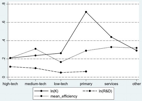
 Table 2 presents the results of eight different models: six of them are estimated across sectors, one for a whole sample and one for an industry. All models are based on Equation (6). Both fixed- and random effect models (the choice is based on the random-effects test in Table 2) are presented. In all models robust standard errors were used. All estimates are derived from multiple tests of a number of options, including combinations of external factors. In addition to sector models, one industry (2423) as a part of the high-tech sector is outlined, as an example, to indicate differences between sector- and industry-based estimates within the same technology category. Differences of similar magnitude between sector averages and industries in the same sector (as in Table 2) were found within all sectors. Using the same example, the mean efficiency of the pharmaceutical industry, estimated within the high-tech sector and with separate production function, is 0.51 versus 0.6. This indicates that R&D intensity, as the basis for grouping, may not always be the most adequate, as indicated already at the creation of this measure (Hatzichronoglou, 1997).

The model estimated for the whole sample has shortcomings: these estimates are generally averages over sectors and sector heterogeneity is largely indistinguishable. As depicted in Table 2, external factors, significant in sector-based models, are mostly non-significant in the whole sample. However, production input estimates are still significant, and some general conclusions can be made, which follow at the end of this subsection. In what follows, we compare sector-based estimates. Concerning the parameter estimates of the input variables, physical capital is statistically significant and important in all sectors. In manufacturing sectors, the elasticity of physical capital depends on the sectors’ technological level, declining steadily with rising technological level. However, the differences between sectors’ highest and lowest elasticities are not so remarkable, at around 20%. In turn, R&D capital elasticity shows the opposite trend, increasing steadily with technical level. Here, the differences between highest and lowest elasticities are significantly larger (0.115 versus 0.05). The difference in technological level has a stronger influence on R&D capital elasticity than on capital elasticity. In all remaining sectors physical capital has a higher elasticity than in manufacturing sectors, being the highest in the primary sector (0.715). The primary sector also differs from other non-manufacturing sectors due to non-zero R&D capital elasticity. This is understandable, since the primary sector also includes agriculture. For example, from global science spending, approximately 5% was spent on agricultural R&D in 2000, and this spending is constantly growing, fed by growth rates of global population (Alston, 2011). Other non-manufacturing sectors are not affected by R&D capital. It is necessary to note that the R&D effect increases, if a particular industry or sector moves closer to the efficiency frontier (Aghion, 2006; Acemoglu, Aghion, & Zilibotti, 2006). In that case the innovation becomes an important source of development, while the importance of imitation decreases. In present models the R&D capital elasticity indicates its impact on the efficiency frontier, therefore for industries located farther away the effect may be lower.

A time trend of technological change across sectors is also clearly pronounced, being the lowest in high-tech and highest in other non-manufacturing industries (2.6% versus 11.1%). The high-tech sector shifts the boundaries, which is more difficult to carry out; other sectors can use the achievements of high-tech for their own development. Only the primary sector shows no progress in technological level,¹⁴ but at the same time the primary sector is the only one with time-varying inefficiency. Therefore, the inefficiency is decreasing, industries in the primary sector are moving closer to the efficiency frontier (on average 4.4% per year).

Such results are generally in accordance with previous studies of a similar type (Tsai & Wang, 2004; Kumbhakar et al., 2012),¹⁵ which, however, were based on firm-level data. For instance, Kumbhakar et al. (2012) found similar trends in input elasticities; also, time trends of technical progress are fairly close in some sectors (2.9% in the high-tech sector and 3.3% in the whole sample). However, this study includes no efficiency comparison across sectors or countries. Tsai and Wang (2004)¹⁶ estimated R&D capital elasticity, but not efficiency. R&D capital elasticity from the present study is also in line (regarding sign and magnitude) with prior studies (e.g. Hall et al., 2010), which, however, are using production function, not SFA. We will not make any closer comparison with other studies, due to differences in estimation methods, scope, and aggregation level of data samples.

Among the external factors used, we consider the share of labour with tertiary education to be most important, as this is a factor that the state can affect. The factor has positive elasticity in high and medium-tech manufacturing, and in services. This factor has an even higher elasticity than R&D capital respectively, in high and medium-tech sectors. Across sectors, the highest elasticity is in the medium-tech sector. In the separately estimated pharmaceutical industry, the positive effect of educated labour is significantly stronger than in all other sectors, which indicates substantial heterogeneity within sectors, larger than between sector averages. It is important to consider here some externalities, related to tertiary education. Tertiary education improves the capacity to develop new technologies, when the innovation becomes the basis of development (Acemoglu et al., 2006; Aghion, 2006). Tertiary education also improves the productivity, when the state is close to the efficiency frontier; this relationship is amplified by the migration of educated labour, from regions with lower productivity¹⁷ (Aghion, Boustan, Hoxby, & Vandenbussche, 2009). Such migration also improves the productivity of high-productive regions, while reducing the potential of low-productive regions.¹⁸ Therefore, regarding tertiary education, various effects should be considered, depending on the efficiency of a particular industry/country.

Other external factors are not generally under government control, so policy options are more restrained. The wider effect from these other factors sees the percentage of Internet users having an impact on the three sectors (medium, low-tech, and services). The impact on the low-tech and service sectors is negative. We also tested all industries separately among these two sectors and despite a parameter variation across industries; the sign is negative in all industries. This may refer to the well-known productivity paradox, that computers are everywhere except productivity statistics (Brynjolfsson, 1993). As already indicated above, the diffusion and spillover use the same channels, and diffusion (spread of technology) cannot be negative. Therefore, this negative effect in low-tech and service sectors may be attributed to spillovers. What exactly these spillovers could be, is not the subject of present study, but one of the hypotheses may be that computers and Internet may be used also for entertainment purposes (e.g. social media).

In contrast to low-tech manufacturing and services, in medium-tech manufacturing the Internet definitely has a positive impact on efficiency. This result was also tested separately among all industries within the medium-tech sector, and in all these industries the Internet has a positive impact. Another communication channel, mobile phones, has a statistically significant impact only in the low-tech sector, and this impact is negative, similar to the Internet impact. The last two external factors are trade of ICT products, their share in total export and import. As mentioned before, exports usually have a smaller impact and the same has been found here. In medium-tech manufacturing it has a lowest elasticity among all factors within this sector. ICT products import has a much larger impact in the primary and other non-manufacturing industries sectors. In the case of the latter sector, the model was also estimated separately by industries and the magnitude of estimated factor parameter was almost similar in all industries. In the last sector, the ICT import factor has (on average) a higher elasticity than physical capital. We can conclude that ICT import has a relatively stronger impact on productivity than ICT export.

Now we return to the whole sample model. The whole sample model is a compromise, aimed at the comparison of directly non-comparable sector efficiencies, because the sector-based mean efficiency (see Table 2) is meaningful only for the relevant sector. Incomparability of sector-based efficiencies is demonstrated by mean efficiencies, where the whole sample has a lower average (∼0.14) than the average over sectors, taken separately (∼0.36). To make a common scale for efficiencies, we compare sectors’ bests with a common best in the whole sample. In this case, the highest efficiency is 1 for a whole sample (see Figure 1). The ratio of the highest efficiency of an arbitrary sector to the highest efficiency of a whole sample gives the scaling factor. Multiplying the scaling factor with the sector-based efficiency of a particular industry gives us the efficiency of that particular industry on a common scale.

Figure 1. The whole sample estimates, comparison of the highest efficiencies across industries.

Source: authors’ calculations.

Such a relationship is however approximate, because across sectors different models (fixed and random effect) are used. In addition, the whole sample model may have some shortcomings (as noted before). The efficiencies converted in such a way can be compared with input elasticities (see Figure 2). According to Figure 2, we can make some additional conclusions, that generally, R&D capital elasticity (as well as R&D intensity) and efficiency are not related.¹⁹ According to Figure 2, services and other non-manufacturing industries have the highest mean efficiency, while R&D capital elasticity is not significant. It can be interpreted that the R&D is an important source of development, but not in the same way across sectors. Some key findings in addition to the above are the following: (1) the grouping of industries by R&D intensity results in too heterogeneous sectors, therefore industry-based models are preferable; (2) R&D intensity has no clear relationship to efficiency. In the following section we narrow our focus to industry level, to examine the efficiency distribution.

Figure 2. Factor input elasticities and efficiency across sectors.

Source: authors’ calculations.

4.2. Efficiency within industries

In this subsection we focus on the industry level. Due to the large number of industries we select only two of them for more detailed investigation, one for main focus and a second for comparison. The choice of industries was based on the R&D capital elasticity; we select two opposites. From the high-tech sector we select the electronics industry (ISIC code 32) (as the main industry under analysis), from others we take mining and quarrying (10–14) (for contrast). The electronics industry is considered the most important among producers of material goods; their products allow productivity gain for other industries and stimulation of innovation in the whole economy (Mann & Kirkegaard, 2006). We use the same models as before, and depict the efficiency within industry across countries (see Figure 3). These two industries have a different efficiency axis, because they do not share a common production possibility frontier (they are estimated with different production functions).

Figure 3. Intra-industry distribution of efficiency in the electronics manufacturing (32) and mining and quarrying (10–14).

Source: authors’ calculations.

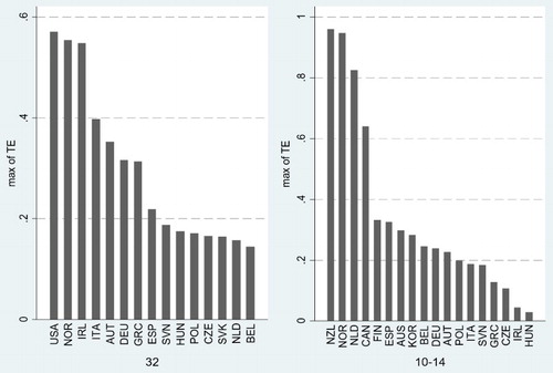
The efficiency of an arbitrarily chosen industry in some particular country is affected by two compound factors: the market power of the firms within this industry (the position in the value chain) and the nature of the market power of the industry (innovative versus non-innovative). According to Figure 3, the efficiency varies significantly within industries across countries, in electronics the countries with the highest and lowest efficiency differ from each other by nearly 3 times and in mining and quarrying by nearly 20 times. Competition should equalize the efficiency, because low-productive producers are dropping out from the market. Based on this, the electronics industry seems significantly more competitive (narrower efficiency interval). At this point it should be remembered that we are using a revenue-based productivity (value added per worker), which includes both price and quantity effects (as noted above). To examine the efficiency distribution in the above noted industries, we need to account for the existence of global value chains.²⁰ The presence of global value chains is very likely the most common in the electronics industry (OECD, 2012). This is mainly due to the product modularity,²¹ which supports fragmentation and geographical diffusion of processes. This, in turn, allows the replacement of the actors of the value chain, without significant changes in the product design or process (Langlois, 2003). All of this affects the actors of the value chains, therefore even the biggest subcontractors have little market power, and they are characterized by fierce competition and low profitability (Sturgeon & Kawakami, 2010). Value added in global value chains is distributed very unevenly in the case of the electronics industry; the largest share of it goes to the chain's lead firm and the lowest to the subcontractors (Dedrick, Kraemer, & Linden, 2010).²² The lead firm may not be the brand owner; much depends on the structure²³ of particular value chain (Sturgeon & Kawakami, 2010). Most lead electronics producers are located in Europe, Japan, the USA, and Korea; subcontractors are mostly in emerging countries.

Generally, the largest share of the value added goes to those who protect themselves from competition, creating barriers to competitors – a higher barrier ensures higher productivity (Kaplinsky &Morris, 2001). Barriers may occur for different reasons, e.g. control over limited natural resources, access to infrastructure or political favour. A significant group is of an endogenous type of barriers, which arise as a result of the firm's activities, allowing a Schumpeterian-type of profit.²⁴ In the case of the electronics industry, higher productivity comes mostly from innovation, because the competition in this sector is fierce. Value added for mining and quarrying is based on factors like exclusive access to limited natural resources, also concentration of market power and supply control (e.g. Organization of the Petroleum Exporting Countries, OPEC) (Stevens, 2005). For example, the global oil market is strongly oligopolistic, which together with external factors allows earning considerable rent.

These noted factors form the efficiency in the previously mentioned industries (Figure 3), resulting in quite different distributions of efficiency. Whereas competition filters out weaker firms, we may assume the price effects are the main reason of (revenue-based) efficiency differences. Within industry the value chain's lead firm shapes the efficiency distribution, due to market power and impact on other actors’ demand. Value chain actors with little market power are representing the above-mentioned combination of high technical efficiency with low value added. Unfortunately, this OECD-based data sample does not contain emerging countries, where most of the subcontractors are located (e.g. China). Otherwise, we could get a significantly wider range of efficiency distribution. For example, with the Apple iPad, Apple's profit amounts to about 30% of the sales price, while labour costs in China's assembly is around 2% of the retail price (The Economist, 2012). However, this aspect does not affect differences in maximum efficiency (see Figure 1) between industries in Figure 3. The differences between industries’ highest efficiency characterizes the influence of different barriers, where factors other than innovation enable the creation of higher barriers and thereby higher value added.

In conclusion, it must be stressed that the precise impact of R&D on the efficiency is not simply and unambiguously estimable. The position of firms in the value chain and the position of value chains in the economy both matter.²⁵ Value chains may be very different and so are relations between chains’ actors which will result in the distribution of value added across chains. This result is somehow opposite to the policy recommendations of Kumbhakar et al. (2012), that supporting the R&D investment shifts the boundaries and increases productivity. This may be so regarding the world economy, but in terms of a particular country it may not work. For example, the high-tech electronics industry in Estonia is represented by a number of subcontractors that offer low value added manufacturing services to the foreign multinationals. Differently, these companies are just production units without any R&D, have little subsidiary autonomy and as such are locked in to captive networks. If they would even have some R&D, which would be supported by the government, then their positions in particular value chains means no net gain for Estonia. To be effective in designing R&D policy measures, one must have a detailed knowledge of the relevant value chain structure and the target company's position in the chain. Without such knowledge, any R&D policy measure could just turn into costs.²⁶

5. Conclusions

In this article we have used an SFA approach for analysing the contribution of production factors (labour, physical capital, R&D capital) to the efficiency of industries with various technological levels. We have compared sectors according to the OECD taxonomy based on R&D intensity (high-tech, medium-tech, low-tech industries), but also services, primary, and other non-manufacturing industries. The above-mentioned sector groups are compared in our analysis in terms of efficiency, but we have also compared industries across countries.

Our results show that high-tech industries on average are associated neither with the higher efficiency or productivity levels. Still, our results show that R&D capital has productivity enhancing effects more in high-tech industries, which has been also shown earlier by Kumbhakar et al. (2012) for European firms. At the same time, investment in production assets (capital accumulation) shows a higher impact on productivity in low-tech sectors. This dichotomy of the relevance of R&D versus capital investment is generally in line with the other sectoral innovation studies (e.g. Pavitt, 1984) showing varying trajectories of technological development in different economic sectors. It seems that the positive effect of R&D inputs on productivity is decreasing in size starting from high-tech, to medium-tech, following primary industries and lastly, this effect is the smallest in low-tech sectors (where accumulated capital investment plays a more relevant role e.g. in the form of machinery and equipment).

It is interesting to see that the efficiency indicator seems to be related to the power of controlling the value chain, in other words to the barriers limiting the access of the competitors to the market thereby enabling the appropriation of higher profits. One possibility to create such barriers is innovation (e.g. through patents, trademarks, etc.), however, it seems not the ‘best’ way according to our data, as other reasons (exclusive access to the natural resources, political impact, etc.) seem to secure more persistent barriers. Therefore, R&D capital is relevant in sectors where the barriers are not sustainable for the longer term.

The Estonian economy generally operates at low levels of efficiency – in most sector groups it is located at the very end of the country list together with other CEE countries. The sectors that we have assessed (unfortunately, high-tech sectors could not be analysed in the case of Estonia), are in some cases yielding only a half of the efficiency levels compared to the OECD median levels. One clear exception is financial intermediation with relatively high efficiency indicator, comprising about 50% of the maximum level in the OECD. It is only natural, that given the above results, R&D investments play a relatively limited role in determining the productivity and efficiency levels of Estonian industries. Our results show that R&D capital has an impact on the sectors high and medium high-tech manufacturing that amounted in 2011 to 27% of Estonian manufacturing value added and 22% of employment (Eurostat data). For comparison the value added shares were 43% in Finland and 49% in Germany. Therefore, R&D enhancing measures are also relevant only for a relatively smaller share of the manufacturing sector in the Baltic states. Though we did not involve Latvia and Lithuania in the analysis, given that the shares of high-tech and medium high-tech manufacturing in total manufacturing employment are even lower in the case of Latvia (9.1% in 2011) and Lithuania (11% in 2011) it can be said that the above conclusions can be extended also to these.

According to the present models, R&D is affecting efficiency frontiers, i.e. firms and industries with highest efficiencies. The concept of innovation means the implementation of something new, which, together with the commercial success, shifts outwards the boundaries of existing frontiers. Relatively low-productive economies are forced by imitation, which is gradually being replaced by innovation, when the economy moves closer to the efficiency frontier. This means that R&D may not be the best option for low-productive industries. This argument is also extremely relevant for innovation policy, as discussed by Havas (2014), for a country with a lower development level (such as the Baltic states) it would be more appropriate to concentrate on improvement of knowledge dissemination and exploitation rather than scientific knowledge creation, towards which the bulk of the R&D (basic research) is targeted. Our study shows that the R&D capital has a different impact across sectors, which should be considered by policy measures. In industries located at low efficiency levels, imitation (incremental innovation) is a main driver, which could be replaced step by step with more radical innovation as the economy is moving towards the technology frontier. Therefore, initially the incentives for capital investments (subsidies, credits, etc.) are in place in such sectors. However, one cannot make an easy conclusion that the high-tech sector is especially appropriate for R&D supporting policy measures. The same industry across countries may have very different efficiency, which shows the position of a particular country in the value chain. R&D affects mainly firms on the efficiency frontier, i.e. the lead firms in the value chain. For policy measures, it is important to have better knowledge about the position and improvement possibilities of the target industry in that particular chain. For establishing new value chains or moving old industries up the ladder, R&D capital investments should be selectively targeted towards areas or activities with bigger potential to internationalization and higher value added. This selective R&D policy would need to be aligned with the respective policies of foreign direct investment and human capital. Policy measures must be internally consistent or the impact could be adverse. Therefore, selective R&D policies need to be aligned with respective policies of human capital.

The share of labour force with higher education seems to be a relevant framework factor determining the efficiency and productivity levels. In Estonia this is affecting sectors comprising 69% of the added value and employment in Estonia. This factor exerts a great positive impact in general, but it can be asymmetric as for economies operating far from the efficiency frontier (like Estonia), it can have also adverse impact in the short term. As the industries are generally far from the frontier where imitation rather than innovation is important, the emigration of the highly educated labour decreases the positive effect of educational investments of the society. This result could also imply that the higher education policy has to be selective in that respect. One option would be to offer privately funded education in the fields with high emigration effects. Although Hazans and Philips (2011) showed that so far the brain drain has not been a feature of the Baltic emigration as medium educated workers (those with secondary education) have been the most likely to move (possibly somewhat reducing the strength of our argument), there is the problem of brain waste due to the over-qualified high-educated movers.

The natural continuation of this study would be the focus on the distribution of efficiency inside the value chains, their affecting factors, and the possible spillover between chain actors. Such knowledge may help in designing effective policy measures especially for small countries, with relatively high costs of inconsistent policies.

Acknowledgements

We are grateful to an anonymous referee, seminar participants in Tartu, and Andrew Rozeik for several comments. The authors take the sole responsibility for all errors and omissions.

Funding

This research has been supported by the European Social Foundation through the Research and Innovation Policy Monitoring Programme; the Estonian Science Foundation Grants [no. 8580 and 8311]; the Estonian Research Agency [project no. IUT20–49 ‘Structural Change as the Factor of Productivity Growth in the Case of Catching up Economies’].

Notes on contributors

Dr Jaan Masso is a Senior Research Fellow at the University of Tartu, Estonia. He received his PhD from the University of Tartu in 2005. His main research areas are labour economics (labour demand, wages, labour market flows, labour market of scientists, firm demographics), foreign direct investments, innovations, science policy, international trade. Dr Jaan Masso is the corresponding author and can be contacted at: [email protected]

Dr Kadri Ukrainski received her PhD in 2008 and has been a researcher at the Faculty of Economics and Business Administration at the University of Tartu, Estonia since 2004. Her main research focus is related to the innovation and respective policy more broadly. She has conducted research in knowledge economics, with particular emphasis on knowledge as a source of innovation; sectoral innovation systems with the focus on low- and medium-technology industries; but also science and innovation policy.

Margo Liik is a PhD student at the Faculty of Economics and Business Administration at the University of Tartu, Estonia. He is also acting as a consultant in private sector. His main research interests are related to the efficiency, in different areas and at different levels.

Notes

1. The relationship between innovation inputs and outputs, but also economic performance and well-being is not trivial, and there could be different efficiencies in turning innovation inputs into innovation outputs, as illustrated e.g. by the so-called Swedish paradox (moderate innovation output despite very high innovation inputs) (Edquist & McKelvey, 1998).

2. For instance, Meriküll, Eamets, and Varblane (2012) showed that industrial structure explained only a relatively small share (c. 15%) of the business R&D expenditures of the Central and Eastern Europe (CEE) countries while this share was much higher for some countries like Estonia (almost 50%). In addition, small open economies naturally have higher expenditure on BERD, as a means of internationalization. However, this is usually driven by a few key companies (oligopolistic effects), which skews the data slightly. See, for example, Dachs, Stehrer, & Zahradnik (2014).

3. It needs to be noted that targets are ambitious partly also because the Lisbon Strategy of the EU set the target of R&D spending to reach 3% in GDP by 2010 in all EU countries. This level was not reached, hence the renewed 3% target forming one of the main five targets of the Europe 2020 strategy adopted in 2010.

4. The STAN dataset included data on all 34 OECD countries and the ANBERD dataset for 29 countries. The final sample includes the following countries: Australia; Austria; Belgium; Canada; Czech Republic; Estonia; Finland; Germany; Greece; Iceland; Ireland; Italy; Israel; Hungary; Luxembourg; Netherlands; New Zealand; Norway; Poland; Portugal; Republic of Korea; Slovakia; Slovenia; Spain; and the USA. The final sample is such due to the missing data in some variables for some of the countries.

5. Using R&D capital as an input is affected by the seminal paper of Griliches (1979) and is justified by the following: (1) R&D takes time, there is a lagged impact of a current period expenditures; (2) past R&D investments are depreciating, after some time they become useless; (3) knowledge in one industry is affected by the knowledge in other industries, there is a knowledge spillover. R&D capital is very similar to the physical capital; the only difference is that it is intangible. Considering only the current period expenditure means that knowledge accumulation is missing, i.e. the lack of personal and organizational memory, which is unrealistic.

6. According to ISIC Rev. 3: high-tech manufacturing industries are 2423, 30, 32, 33, 353; low-tech are 15–19, 20–22 and 36–37; medium-tech are all the rest of the range 15–37 (OECD, 2011).

7. R&D intensity is measured as a proportion of R&D expenditures in output.

8. This division is based on the proportion of labour force with tertiary education.

9. Characterized by the spread of new technology, binds both the supply and demand (Stoneman & Battisti, 2010).

10. Externalities of diffusion are called spillovers (Keller, 2010).

11. These products include telecommunication, audio and video equipment, computers and related equipment, electronic components (except software).

12. These are subscriptions to a public mobile telephone service using cellular technology, which provide access to the public switched telephone network, including post-paid and pre-paid subscriptions.

13. The authors also tested Greene's ‘true fixed’ effect model, which shows that almost all industries are efficient.

14. The authors tested two models, with time-varying and time-invariant inefficiency. The time-varying model was statistically better, but the difference was not very significant. The time-invariant model shows technical progress of about 2% per year.

15. The data sample was based on manufacturing industries (577 top European R&D investors) and physical capital had no impact in the high-tech sector.

16. They use only two groups of firms – high-tech electronics and other manufacturing firms.

17. The reason for this is the wage difference between the low and high-productive regions.

18. Aghion et al. (2009) examined the impact of federal funding of tertiary education, with respect to the labour productivity in 48 US states, depending on the distance from the efficiency frontier. Similar funding has a different impact on the productivity: positive in high-productive states, negative in low-productive states.

19. Such a conclusion could be already made according to the whole sample model (see Table 2), where R&D capital elasticity was not significant.

20. The value chain is all those activities, from product concept to production, including support services, which are needed to supply product or service to final customer (Kaplinsky & Morris, 2001).

21. Modularity is one of the key factors, promoting a chain globalization (Jacobides, 2008; Sturgeon, 2002).

22. In fact this is not unique to the electronics sector, but rather typical of sectors which utilize intermediate products to assemble a final product (i.e. most manufacturing sectors). The automotive sector operates in exactly the same way (we thank Andre Rozeik for that comment).

23. A major player could also be a platform-leader, for example Intel (hardware) and Microsoft (software) in PC manufacturing.

24. This is an additional gain that occurs as a result of innovation.

25. A close conclusion has also been made by Lehto, Böckerman, and Huovari (2011), who found that the R&D effect is conditional on the location of firms relative to the efficiency frontier. The effect decreases when the firm moves further away from the frontier.

26. Basically the issue is the governance of the global value chains (see e.g. Gereffi, Humphrey, & Sturgeon, 2005).

References

- Acemoglu, D., Aghion, P., & Zilibotti, F. (2006). Distance to frontier, selection, and economic growth. Journal of European Economic Association, 4, 37–74. doi: 10.1162/jeea.2006.4.1.37
- Aghion, P. (2006). A primer on innovation and growth (The Bruegel Policy Brief Issue 2006/06). Brussels: Bruegel. Retrieved April 14, 2014, from http://www.bruegel.org/publications/publication-detail/publication/233-a-primer-on-innovation-and-growth/
- Aghion, P., Boustan, L., Hoxby, C., & Vandenbussche, J. (2009). The causal impact of education on economic growth: Evidence from the United States (Brookings Papers on Economic Activity, Spring 2009), Conference Draft. Retrieved October 14, 2014, from http://www.brookings.edu/economics/bpea/~/media/Files/Programs/ES/BPEA/2009_spring_bpea_papers/2009_spring_bpea_aghion_etal.pdf
- Aigner, D. J., Lovell, C. A. K., & Schmidt, P. (1977). Formulation and estimation of stochastic frontier production function models. Journal of Econometrics, 6, 21–37. doi: 10.1016/0304-4076(77)90052-5
- Alston, J. M. (2011). Global and U.S. trends in agricultural R&D in a global food security setting, OECD Conference on Agricultural Knowledge Systems: Responding to Global Food Security and Climate Change Challenges, OECD. Retrieved from http://www.oecd.org/tad/agricultural-policies/48165448.pdf
- Baltagi, B. H. (2001). Econometric Analysis of Panel Data (2nd ed.). Chichester: John Wiley & Sons.
- Battese, G., & Coelli, T. J. (1988). Prediction of firm-level technical efficiencies with a generalized frontier production function and panel data. Journal of Econometrics, 38, 387–399. doi: 10.1016/0304-4076(88)90053-X
- Battese, G. E., & Coelli, T. J. (1992). Frontier production functions, technical efficiency and panel data: With application to paddy farmers in India. Journal of Productivity Analysis, 3(1/2), 153–169. doi: 10.1007/BF00158774
- Blomström, M., Lipsey, R., & Zejan, M. (1994). What explains growth in developing countries? In W. Baumol, R. Nelson, & E. Wolff, (Eds.), Convergence of productivity: Cross-national studies and historical evidence (pp. 243–259). Oxford and New York: Oxford University Press.
- Brynjolfsson, E. (1993). The productivity paradox of information technology. Communications of the ACM, 36(12), 66–77. doi: 10.1145/163298.163309
- Chaminade, C., & Edquist, C. (2010). Rationales for public policy intervention in the innovation process: Systems of innovation approach. In S. Kuhlmann, P. Shapira, & R. Smits (Eds.), The theory and practice of innovation policy. An international research handbook (pp. 95–114). Cheltenham: Edward Elgar Publishing.
- Cincera, M., Czarnitzki, D., & Thorwarth, S. (2009). Efficiency of public spending in support of R&D activities, European commission (Economic Papers No. 376). Retrieved October 13, 2014, from http://ec.europa.eu/economy_finance/publications/publication14769_en.pdf
- Coelli, T. J., Rao, D. S. P., O'Donnell, C. J., & Battese, G. E. (2005). An introduction to efficiency and productivity analysis (2nd ed.). New York: Springer.
- Cornwell, C., Schmidt, P., & Sickles, R. (1990). Production frontiers with cross-sectional and time-series variation in efficiency levels. Journal of Econometrics, 46, 185–200. doi: 10.1016/0304-4076(90)90054-W
- Crépon, B., Duguet, E., & Mairesse, J. (1998). Research and development, innovation and productivity: An econometric analysis at the firm level. Journal of Econometrics, 7(2), 115–158.
- Dachs, B., Stehrer, R., & Zahradnik, G. (Eds.). (2014). The internationalisation of business R&D. Cheltenham: Edward Elgar.
- David, P. A., Hall, B. H., & Toole, A. A. (2000). Is public R&D a complement or substitute for private R&D. Research Policy, 29(4–5), 497–529. doi: 10.1016/S0048-7333(99)00087-6
- Dedrick, J., Kraemer, K. L., & Linden, G. (2010). Who profits from innovation in global value chains?: A study of the iPod and notebook PCs. Industrial and Corporate Change, 19(1), 81–116. doi: 10.1093/icc/dtp032
- The Economist. (2012, January 21). The trade gap between America and China is much exaggerated. Retrieved February 20, 2014, from http://www.economist.com/node/21543174
- Edquist, C., Malerba, F., Metcalfe, J. S., Montobbio, F., & Steinmueller, W. E. (2004). Sectoral systems: Implications for European innovation policy. In F. Malerba (Ed.), Sectoral systems of innovation: Concepts, issues and analyses of six major sectors in Europe (pp. 427–461). Cambridge: Cambridge University Press.
- Edquist, C., & McKelvey, M. (1998). High R&D intensity without high tech products: A Swedish Paradox? In N. Klaus, & B. Johnson (Eds.), Institutions and economic change: New perspectives on markets, firms and technology (pp. 131–149). Cheltenham: Edward Elgar Publishing Ltd.
- Eurostat. (2014). Glossary: Knowledge-intensive services. Retrieved February 10, 2012, from http://epp.eurostat.ec.europa.eu/statistics_explained/index.php/Glossary:Knowledge-intensive_services_%28KIS%29
- Fagerberg, J., Srholec, M., & Verspagen, B. (2010). Innovation and economic development. In B. H. Hall & N. Rosenberg (Eds.), Handbook of the economics of innovation (pp. 833–873). Elsevier.
- Falk, R., & Leo, H. (2006). What can be achieved by special R&D funds when there is no special leaning towards R&D intensive industries? (WIFO Working Paper No. 273/2006). Retrieved October 11, 2014, from http://www.wifo.ac.at/en/publications/working_papers?detail-view=yes&publikation_id=26621
- Foster, L., Haltiwanger, J., & Syverson, C. (2008). Reallocation, firm turnover, and efficiency: Selection on productivity or profitability? American Economic Review, 98, 394–425. doi: 10.1257/aer.98.1.394
- Gereffi, G., Humphrey, J., & Sturgeon, T. (2005). The governance of global value chains. Review of International Political Economy, 12(1), 78–104. doi: 10.1080/09692290500049805
- Greene, H. W. (2005). Reconsidering heterogeneity in panel data estimators of the stochastic frontier model. Journal of Econometrics, 126, 269–303. doi: 10.1016/j.jeconom.2004.05.003
- Greene, H. W. (2007). Econometric analysis (6th ed.). Upper Saddle River, N.J.: Pearson Prentice Hall.
- Greene, H. W. (2008). The econometric approach to efficiency analysis. In H. O. Fried, C. A. K. Lovell, & S. S. Schmidt (Eds.), The measurement of productive efficiency and productivity growth (pp. 92–250). Oxford: Oxford University Press.
- Greene, W. (1990). A gamma-distributed stochastic frontier model. Journal of Econometrics, 46, 141–163. doi: 10.1016/0304-4076(90)90052-U
- Griffith, R., Redding, S., & Van Reenen, J. (2004). Mapping the two faces of R&D: Productivity growth in a panel of OECD industries. Review of Economics and Statistics, 86, 883–895. doi: 10.1162/0034653043125194
- Griliches, Z. (1979). Issues in assessing the contribution of R&D to productivity growth. The Bell Journal of Economics, 10(1), 92–116. doi: 10.2307/3003321
- Guan, J., & Chen, K. (2010). Measuring the innovation production process: A cross-region empirical study of China's high-tech innovations. Technovation, 30, 348–358. doi: 10.1016/j.technovation.2010.02.001
- Guellec, D., & van Pottelsberghe, B. (2003). The impact of public R&D expenditures on business R&D. Economics of Innovation and New Technologies, 12(3), 225–244. doi: 10.1080/10438590290004555
- Hall, B. H. (2011). Innovation and productivity. In J. B. Madsen & A. Sørensen (Eds.), Nordic Economic policy review, 2(2011), 167–203.
- Hall, B. H., Mairesse, J., & Mohnen, P. (2010). Measuring the returns to R&D. In B. H. Hall & N. Rosenberg (Eds.), Handbook of the economics of innovation (Vol. 2, pp. 1033–1082). Elsevier.
- Hatzichronoglou, T. (1997). Revision of the high- technology sector and product classification (OECD Science, Technology and Industry Working Papers), OECD Publishing. Retrieved February 10, 2014, from http://dx.doi.org/10.1787/134337307632
- Havas, A. (2014). Trapped by the high-tech myth: The need and chances for a new policy rationale. In H. Hirsh-Kreinsen & I. Schwinge (Eds.), Knowledge-intensive entrepreneurship in low-tech sectors: The prospects of traditional economic INDUSTRIES (pp. 193–217). Cheltenham: Edward Elgar.
- Hazans, M., & Philips, K. (2011). The post-enlargement migration experience in the Baltic labor markets. In M. Kahanec & K. F. Zimmermann (Eds.), EU Labor markets after post-enlargement migration (pp. 255–304). Berlin-Heidelberg: Springer.
- Henry, M., Kneller, R., & Milner, C. (2009). Trade, technology transfer and national efficiency in developing countries. European Economic Review, 53(2), 237–254. doi: 10.1016/j.euroecorev.2008.05.001
- Higon, D. A., Manez, J. A., & Sanchis-Llopis, J. A. (2011). The role of extensive and intensive margins in explaining corporate R&D growth: Evidence from Spain (Instituto Valenciano de Investigaciones Económicas Working Papers no. EC 2011–05). Retrievd October 12, 2014, from http://www.ivie.es/downloads/docs/wpasec/wpasec-2011-05.pdf
- Jacobides, M. G. (2008). Playing football in a soccer field: Value Chain structures, institutional modularity and success in foreign expansion. Managerial and Decision Economics, 29, 257–276. doi: 10.1002/mde.1393
- Jaumotte, F., & Pain, N. (2005). From ideas to development: The determinants of R&D and patenting (OECD Economics Department Working Papers No. 44). Retrieved October 13, 2014, from http://www.oecd.org/officialdocuments/publicdisplaydocumentpdf/?doclanguage=en&cote=ECO/WKP(2005) 44
- Johansson, B., Lööf, H., & Ebersberger, B. (2008). The innovation and productivity effect of foreign take-over of national assets. CESIS Electronic Working Paper No. 141.
- Jondrow, J., Lovell, C. A. K., Materov, I. S., & Schmidt, P. (1982). On the estimation of technical inefficiency in the stochastic frontier production function model. Journal of Econometrics, 19, 2323–238. doi: 10.1016/0304-4076(82)90004-5
- Kancs, d'A., & Siliverstovs, B. (2012). R&D and non-linear productivity growth of heterogeneous firms (European Commission, Joint Research Centre, Institute for Prospective Technological Studies (IPTS), IPTS Working Paper on Corporate R&D and Innovation No. 06/2012).
- Kaplinsky, R., & Morris, M. (2001). A handbook for value Chain research. Prepared for the International Development Research Centre (IDRC). Retrieved February 10, 2014, from http://www.globalvaluechains.org/docs/VchNov01.pdf
- Keller, W. (2010). International trade, foreign direct investment, and technology spillovers. In B. H. Hall & N. Rosenberg (Eds.), Handbook of the economics of innovation (Vol. 2, pp. 1033–1082). Elsevier.
- Kneller, R., & Stevens, P. (2006). Frontier technology and absorptive capacity: Evidence from OECD manufacturing industries. Oxford Bulletin of Economics and Statistics, 68(1), 1–21. doi: 10.1111/j.1468-0084.2006.00150.x
- Kohler, U., & Kreuter, F. (2005). Data analysis using stata. College Station TX, USA: Stata Press.
- Konkurentsivõime kava ‘Eesti 2020’. (2011). Retrieved September 22, 2014, from http://ec.europa.eu/europe2020/pdf/nrp/nrp_estonia_et.pdf
- Koop, G. (2001). Cross-sectoral patterns of efficiency and technical change in manufacturing. International Economic Review, 42(1), 73–103. doi: 10.1111/1468-2354.00101
- Kumbhakar, S. C. & Lovell, C. A. K. (2000). Stochastic frontier analysis. Cambridge: Cambridge University Press.
- Kumbhakar, S. C., Ortega-Argilés, R., Potters, L., Vivarelli, M., & Voigt, P. (2012). Corporate R&D and firm efficiency: Evidence from Europe's top R&D investors. Journal of Productivity Analysis, 37, 125–140. doi: 10.1007/s11123-011-0223-5
- Langlois, R. N. (2003). The vanishing hand: The changing dynamics of industrial capitalism. Industrial and Corporate Change, 12(2), 351–385. doi: 10.1093/icc/12.2.351
- Lee, H.-Y., Park, Y.-T. (2005). An international comparison of R&D efficiency: DEA approach. Asian Journal of Technology Innovation, 13(2), 207–222. doi: 10.1080/19761597.2005.9668614
- Lehto, E., Böckerman, P., & Huovari, J. (2011). The return to the technological frontier: The conditional effect of R&D on plant productivity in Finnish manufacturing. Papers in Regional Science, 90(1), 91–109. doi: 10.1111/j.1435-5957.2010.00318.x
- Lithuania: National Reform Programme 2013. (2013). Vilnius. Retrieved September 22, 2014, from http://ec.europa.eu/europe2020/pdf/nd/nrp2013_lithuania_en.pdf
- Mairesse, J., & Mohnen, P. (2010). Using innovation surveys for econometric analysis. In B. H. Hall & N. Rosenberg. (Eds.), Handbook of the economics of innovation (pp. 1130–1155). Amsterdam: Elsevier.
- Mandl, U., Dierx, A., & Ilzkovitz, F. (2008). The effectiveness and efficiency of public spending (Economic Papers No 301). European Commission. Retrieved October 13, 2014. from http://ec.europa.eu/economy_finance/publications/publication11902_en.pdf
- Mann, C. L., & Kirkegaard, J. F. (2006). Accelerating the globalization of America: The role for information technology. Peterson Institute Press: All Books, Peterson Institute for International Economics, number 3900.
- Masso, J., Liik, M., & Ukrainski, K. (2013). Teaduse-arendustegevuse ja innovatsiooni indikaatorid Eesti innovatsiooni- ja teaduspoliitikas: senine praktika ja poliitikasoovitused, Teadus- ja Innovatsioonipoliitika Seire Programm, Uuringu 7.1 raport. Retrieved from http://tips.ut.ee/index.php?module=32&op=1&id=3613
- Meeusen, W., & van den Broeck, J. (1977). Efficiency estimation from Cobb-Douglas production functions with composed error. International Economic Review, 18, 435–444. doi: 10.2307/2525757
- Meriküll, J., Eamets, R., & Varblane, U. (2012). Knowledge creation in central and Eastern Europe: The role of sectoral composition. In E. Carayannis, U. Varblane, & T. Roolaht (Eds.), Innovation systems in small catching-up economies: New perspectives on practice and policy (pp. 59–77). Springer-Verlag.
- OECD. (2011). ISIC Rev. 3 technology intensity definition, OECD Directorate for Science, Technology and Industry. Retrieved July 15, 2013, from http://www.oecd.org/sti/ind/48350231.pdf
- OECD. (2012). Mapping global value Chains. Retrieved February 15, 2014, from http://www.oecd.org/dac/aft/MappingGlobalValueChains_web_usb.pdf
- OECD. (2014). Education. OECD better life index. Retrieved February 15, 2014, from http://www.oecdbetterlifeindex.org/topics/education/
- Pavitt, K. (1984). Sectoral patterns of technical change: Towards a taxonomy and a theory. Research Policy, 13(6), 343–374. doi: 10.1016/0048-7333(84)90018-0
- Pessoa, A. (2010). R&D and economic growth: How strong is the link? Economics Letters, 107, 152–154. doi: 10.1016/j.econlet.2010.01.010
- Rousseau, S., & Rousseau, R. (1997). Data envelopment analysis as a tool for constructing scientometric indicators. Scientometrics, 40(1), 45–56. doi: 10.1007/BF02459261
- Savvides, A., & Stengos, T. (2009). Human capital and economic growth. Stanford: Stanford University Press.
- Schibany, A., & Streicher, G. (2008). The European innovation scoreboard: Drowning by numbers? Science and Public Policy, 35(10), 717–732. doi: 10.3152/030234208X398512
- Schmidt, P., & Sickles, R. C. (1984). Production frontiers and panel data. Journal of Business and Economic Statistics, 2(4), 367–374.
- Stevens, P. (2005). Oil markets. Oxford Review of Economic Policy, 21(1), 19–42. doi: 10.1093/oxrep/gri002
- Stevenson, R. (1980). Likelihood functions for generalized stochastic frontier estimation. Journal of Econometrics, 13, 57–66. doi: 10.1016/0304-4076(80)90042-1
- Stoneman, P., & Battisti, G. (2010). The diffusion of new technology. In B.H. Hall & N. Rosenberg (Eds.), Handbook of the economics of innovation (Vol. 2, pp. 733–760). Elsevier.
- Sturgeon, T. (2002). Modular production networks: A new American model of industrial organization. Industrial and Corporate Change, 11(3), 451–496. doi: 10.1093/icc/11.3.451
- Sturgeon, T. J., & Kawakami, M. (2010). Global value chains in the electronics industry: Was the crisis a window of opportunity for developing countries? World Bank Policy Research Working Paper No. 5417.
- Syverson, C. (2011). What determines productivity? Journal of Economic Literature, 49(2), 326–365. doi: 10.1257/jel.49.2.326
- Teece, D. J. (2010). Technological innovation and the theory of the firm: the role of enterprise-level knowledge, complementarities, and (dynamic) capabilities. In B. H. Hall & N. Rosenberg (Eds.), Handbook of the economics of innovation (Vol. 1, pp. 679–730). Elsevier.
- Tsai, K. H., & Wang, J. C. (2004). R&D productivity and the Spillover effects of high-tech industry on the traditional manufacturing sector: The case of Taiwan. World Economy, 27, 1555–1570. doi: 10.1111/j.1467-9701.2004.00666.x
- Ukrainski, K., Kanep, H., & Masso, J. (2013). Eesti teaduse rahastamise rahvusvaheline võrdlevanalüüs, Teadus- ja Innovatsioonipoliitika Seire Programm, Uuringu 2.1 raport. Retrieved from http://www.tips.ut.ee/index.php?module=32&op=1&id=3561
- Wang, E. C. (2007). R&D efficiency and economic performance: A cross-country analysis using the stochastic frontier approach. Journal of Policy Modelling, 29, 345–360. doi: 10.1016/j.jpolmod.2006.12.005
- Wang, E. C., & Huang, W. (2007). Relative efficiency of R&D activities: A cross-country study accounting for environmental factors in the DEA approach. Research Policy, 36, 260–273. doi: 10.1016/j.respol.2006.11.004
- White, H. (1980). A heteroscedasticity-consistent covariance matrix estimator and a direct test for heteroscedasticity. Econometrica, 48, 817–838. doi: 10.2307/1912934
- Wooldridge, M. J. (2010). Econometric analysis of cross section and panel data (2nd ed.). Cambridge, Massachussets, England: The MIT Press.
- Xu, B. (2000). Multinational enterprises, technology diffusion, and host country productivity growth. Journal of Development Economics, 62, 477–493. doi: 10.1016/S0304-3878(00)00093-6
- Zhang, A. Z., Zhang, Y., & Zhao, R. (2003). A study of the R&D efficiency and productivity of Chinese firms. Journal of Comparative Economics, 31, 444–464. doi: 10.1016/S0147-5967(03)00055-6
- Zhang, M. (2012). The comparison of stochastic frontier analysis with panel data models (Doctoral Thesis). Loughborough University, Leicestershire, UK. Retrieved July 5, 2013, from https://dspace.lboro.ac.uk/dspace-jspui/handle/2134/9643