The equilibrium real exchange rate: pros and cons of different approaches with application to Latvia

Abstract

This paper studies various approaches to the equilibrium real effective exchange rate estimation, including structural and direct estimation approaches. It shows their strengths and weaknesses with application to the case of Latvia. Despite the approaches differing considerably in terms of their theoretical background and data used they all indicate that the real exchange rate of Latvia after appreciation during the boom years and subsequent adjustment afterwards remained close to its equilibrium level at the end of the sample period, namely at the end of 2010.

Keywords:

• BEER
• FEER
• Latvia
• NATREX
• SVAR

JEL Classification:

• F31
• F32
• O24

1. Introduction

Real exchange rate is an important macroeconomic concept which reflects movements in relative prices. It is essential that the real exchange rate does not depart significantly and persistently from its equilibrium level determined by economic fundamentals so that relative prices remain close to equilibrium over time and a country's external position is sustainable. However, the equilibrium real exchange rate is not directly observable and requires to be estimated with appropriate models.

This study sets out to estimate the equilibrium real effective exchange rate (REER) of Latvia by employing a bunch of different approaches. Over the past decades, Latviàs economy experienced substantial economic transformations. Accumulation of internal and external imbalances after joining the EU was followed by a severe economic crisis and economic adjustment. The REER has also undergone significant movements from appreciation in the boom years to subsequent depreciation in the recession period. These developments warrant an assessment of the equilibrium real exchange rate of Latvia to find out whether the headline real exchange rate remains close to its equilibrium after the adjustments that followed the crisis.

The concept of the equilibrium REER is very difficult to pin down and there is a bunch of possible approaches one can apply. Broadly speaking one can distinguish between structural approaches, which explicitly refer to the concept of macroeconomic (internal and external) balance, and reduced-form models that estimate movements in the REER directly as a function of economic fundamentals. In our study we apply both types of approaches. First we use the direct estimation approaches: the behavioural equilibrium exchange rate (BEER) approach suggested by Clark and MacDonald (1998) and the approach based on structural vector autoregressions (SVAR) associated with Clarida and Gali (1994). The former explains actual behaviour of the REER in the cointegrating framework and then applies estimated coefficients of a cointegrating relationship to long-term values of economic fundamentals. The SVAR methodology, in turn, aims at decomposing real exchange rate into permanent and transition components by identifying the supply, demand, and nominal shocks using a long-run identification scheme, and then assessing the equilibrium exchange rate by assuming that only the supply (or supply and demand) shock affects REER in the long run. Second we employ several approaches rooted in structural models: the macroeconomic balance (MB) approach and the external sustainability (ES) approach. These are used by the IMF and stem from the concept of fundamental equilibrium exchange rate (FEER) developed by Williamson (1983). We augment our analysis with the natural real exchange rate (NATREX) approach mainly associated with a numerous studies by Stein (e.g. Stein (1994)), whereby NATREX is the REER that equates the current account balance consistent with full employment to the difference between desired savings and investment.

Despite the approaches differing considerably in terms of their theoretical background and data used our results indicate that the real exchange rate of Latvia after appreciation during the boom years and subsequent adjustment afterwards remained close to its equilibrium level at the end of the sample period, namely at the end of 2010.

The structure of this study is as follows. Section 2 lays out the overview of the equilibrium real exchange rate estimation approaches used in this study. Section 3 presents the estimates of Latviàs equilibrium REER by using direct estimation approaches, namely, the approach BEER and the SVAR approach. In Section 4 estimates of structural approaches (MB, ES, and NATREX) are provided. Section 5 provides comparative analysis of the estimates stemming from five different approaches. Section 6 concludes.

2. Overview of equilibrium REER estimation approaches

Generally all approaches aimed at assessing the equilibrium real exchange rate could be divided into two broad groups: the direct estimation approaches where the equilibrium real exchange rate is obtained by estimating reduced-form equations with real exchange rate specified as a function of fundamental determinants and the approaches involving structural models where the equilibrium exchange rate reconciles internal and external macroeconomic balances.

2.1. Direct estimation approaches to equilibrium REER assessment

The most popular representation of direct estimation approaches is the BEER approach. It rests on direct econometric estimation of the equilibrium real exchange rate using the following reduced-form equation:(1) where Z_1t is a vector of economic fundamentals having effect on the REER in the long run and Z_2t denotes a vector of economic fundamentals having an effect on the REER in the medium term, while T_t is a transitory short-term component, ε_t is a random disturbance term, β₁, β₂, and τ are vectors of reduced-form coefficients. This approach allows capturing short-term movements in the REER by including behavioural factors affecting the REER in model specification.

In a seminal paper on the BEER approach Clark and MacDonald (1998) distinguish two types of misalignment, namely current and total misalignments.

Current misalignment is the difference between the actual REER and the REER given by the current values of the medium- and long-term fundamentals q':(2)

Due to the fact that the medium- and long-term fundamentals may divert from their sustainable or equilibrium levels, which are denoted by and , Clark and MacDonald (1998) also define the total misalignment:(3)

Using Equations (2) and (3), total misalignment can be written as:(4) where transitory factors and the deviation of medium- and long-run determinants from their equilibrium levels are taken into account. In practice, the cointegration technique is used to find long-run relationship between the REER and economic fundamentals.

In this study we also make use of the structural vector autoregression (VAR) approach, which emphasizes the impact of shocks by decomposing movements in the REER into nominal, demand, and supply shocks.

Both approaches, while being of purely statistical nature, do not refer to the notion of macroeconomic balance; thus it is not clear if the equilibrium REERs are in line with internal and external balance. These considerations are however identified in the structural approaches explained below. Also in contrast to structural approaches both the BEER and the SVAR approach help to identify the factors which contribute to the misalignment.

2.2. Structural approaches to equilibrium REER assessment

The most popular representation of structural approaches is the FEER approach. Introduced by Williamson (1983), the FEER is the REER consistent with macroeconomic (more specifically, internal, and external) balance whereby the current account (when economy operates at its potential) is made equal with a sustainable capital account position.(5) where the REER is defined as , y_t denotes aggregate demand, NFA_t is the notation for net foreign assets, and i_t is the interest rate. A bar denotes a long-run/sustainable level of a variable. Superscript st means structural capital flows. In order to obtain the estimate of the FEER one needs to assess the current account balance associated with full employment as well as to define a sustainable capital account position, that is, the one which excludes speculative capital flows and thus is determined by fundamentals. This represents a form of normative analysis whereby the difference between desired aggregate saving and investment (S–I) could be used as a proxy for the equilibrium capital account balance. The equilibrium levels of savings and investment are estimated as functions of various macroeconomic and demographic variables. In this study we apply two different approaches (macroeconomic balance and ES approach) rooted in the FEER methodology. Both of them are used by the IMF in their assessment of a country's external balance and equilibrium REER.¹

Another structural approach we employ is the NATREX approach, which is closely related to the FEER. It imbeds both stock and flow equilibrium conditions. However there is no notion of current account balance associated with full employment embodied in the NATREX method.

3. Direct estimation approaches

3.1. The beer approach

The BEER approach to exchange rate assessment involves three stages. First, we estimate the reduced-form REER equation based on the Latvian macroeconomic series. Second, by using the coefficients estimated in the first stage, we calculate the equilibrium real exchange rate. The coefficients could be applied both to the actual values of regressors (resulting in the so-called current BEER) and to their cyclically adjusted values (the long-term BEER). Third, we derive the gap between the actual REER and the long-term BEER estimated in stage 2. We interpret this gap as the REER misalignment.

In choosing REER determinants, we follow the IMF (2006), Lee, Milesi-Feretti, Ostry, Prati, and Ricci (2008) and Bussière, Ca'Zorzi, Chudik, and Dieppe (2010), that also include a comprehensive review of literature on medium- to long-run factors determining the equilibrium real exchange rate. Below we summarize a variety of possible determinants of equilibrium real exchange rate.

3.1.1. Net foreign assets

If a country is in a debtor's position, net interest payments weigh on the current account balances. These should be compensated for by improved trade balance. The latter requires strengthening the international price competitiveness and a more depreciated real exchange rate.

3.1.2. Fiscal balance

An increase in the budget balance associated with restrictive fiscal policies leads to a rise in national savings, a weaker domestic demand and, thus, real depreciation.

3.1.3. Productivity differential

The effect of productivity differential on the real exchange rate is expected to follow the Balassa–Samuelson theory, which states that if productivity in the tradables sector grows faster than in the non-tradables sector, the resulting higher wages in the tradables sector will put upward pressure on wages in the non-tradables sector, leading to higher relative prices of non-tradables and, thus, real appreciation.

3.1.4. Investment ratio

Higher investment ratio is expected to raise productivity leading to real appreciation of currency.

3.1.5. Commodity terms of trade

It is expected that higher commodity terms of trade should lead to real exchange rate appreciation via real income effect.

3.1.6. Openness to trade

Countries with higher total trade-to-GDP ratio (proxy for openness to international trade) are subject to tougher competition in international markets and smaller prices of tradables. This leads to more depreciated currencies.

3.1.7. Government consumption to GDP

An increase in government consumption biased towards nontradables as a ratio of GDP is likely to increase relative prices of nontradable goods and lead to real exchange rate appreciation.

In this study, quarterly data covering the period from the first quarter of 2001 to the fourth quarter of 2010 are used. The choice of the period is dictated by the absence of some of the variables for earlier years on the one hand, and structural changes of Latvia's economy that took place right after the Russian crisis when Latvia switched away from Commonwealth of Independent States (CIS) markets towards European markets on the other. As to the structural changes, a significant shift in external trade pattern was represented by a change in Latvia's merchandise export share to the CIS countries that before the Russian financial crisis had stood between 35% and 45% and quickly declined to around 10–15% after it. Given that lagged foreign trade weights are used in the REER calculations and the switch of external trade towards more developed markets was likely to carry with it also a change in quality of exported goods, these developments may have distorted the REER data, and they may, to some extent, mask the underlying developments of real exchange rate at that time.

Most variables (except for net foreign assets and terms of trade) are calculated as deviations from the respective weighted average values for Latvia's major trading partners Denmark, Germany, Estonia, France, Italy, Lithuania, the Netherlands, Poland, Finland, Sweden, and the UK. All variables have been seasonally adjusted by census X12.

We do not have robust evidence of the stationarity of the REER and its determinants as shown by the unit root test results.² At the same time, for these variables in the first differences, the null hypothesis of a unit root can be rejected, implying that all these variables (along with the REER itself) appear to be integrated of order one, and there is a possibility of cointegration relationship between them. Therefore it is possible to assume the existence of the time-varying exchange rate equilibrium, which can be represented by cointegration relationship between the real exchange rate and its determinants.

Cointegration analysis is carried out by running VECMs and applying the Johansen procedure. We estimate 256 VECM specifications for all possible subsets of 3–7 variables with different number of lags. We identify 21 VECMs containing cointegrating vectors for the REER with theoretically plausible signs. However, only four of them pass the diagnostic tests on normality, heteroskedasticity, and serial correlation of residuals, and contain statistically significant (at 5% reference value) cointegrating parameters (see Table 1).

Table 1. Estimation of VECMs for reduced-form REER equation^a.

	Variable	VECM1	VECM2	VECM3	VECM4
	constant	5.210	4.944	3.750	4.409
Long-run parameters	Productivity differential	0.267 (2.067)	–	0.752 (4.193)	0.825 (5.560)
	Total trade to GDP ratio	–0.012 (–11.416)	–	–	–0.008 (–8.191)
	Net foreign assets	–	0.109 (1.908)	–	–
	Terms of trade	–	–	1.685 (3.706)	1.176 (2.975)
	Fiscal balance to GDP ratio	–	–0.052 (–8.553)	–0.031 (–7.162)	–
Adjustment coefficients	Exchange rate	–0.089 (–0.769)	–0.002 (–0.027)	0.080 (0.973)	0.078 (0.743)
	Productivity differential	–0.014 (–0.054)	–	0.551 (3.793)	0.683 (3.474)
	Total trade to GDP ratio	–95.553 (–3.858)	–	–	–50.880 (–1.978)
	Net foreign assets	–	0.004 (0.043)	–	–
	Terms of trade	–	–	–0.019 (–0.305)	0.022 (0.304)
	Fiscal balance to GDP ratio	–	–28.070 (–5.408)	–20.806 (–2.644)	–
Diagnostic tests	Serial correlation test	9.702 [0.375]	6.442 [0.695]	6.387 [0.983]	21.823 [0.149]
	Normality test	7.207 [0.302]	11.196 [0.083]	12.377 [0.135]	11.810 [0.160]
	Heteroskedasticity test	99.690 [0.131]	50.480 [0.376]	168.651 [0.717]	180.124 [0.483]

Source: authors’ estimates.

^at-statistic values for long-run parameters and adjustment coefficients are provided in parenthesis, probability levels for diagnostic tests are placed in square brackets.

The trace tests³ show that there is at least one cointegrating relationship in the models chosen, while the second cointegrating relationship is only marginally significant in VECM1 and VECM2. We therefore focus on the specification with only one cointegrating relationship (we cannot reject the existence of at most one cointegrating relationship at the 1% level for all chosen specifications).

The estimated VECM1 shows that movements in the REER are correlated positively with the developments in productivity differential vis-à-vis trading partners and negatively with the degree of openness. We identify the statistical significance of productivity differential in three VECMs out of four chosen, while the total trade to GDP ratio appears to be statistically significant in only two of them. By contrast in VECM2, the real exchange rate is correlated positively with the net foreign assets and negatively with the fiscal balance to GDP ratio. It should be noted that none of the VECMs identifies statistical significance of the investment ratio and government consumption ratio in a long-run relationship for the REER.

What seems to be striking is the fact that the adjustment coefficients for the REER are not significant in any VECM specification, namely the gap between the actual and the equilibrium REER is not closed by an adjustment in the REER itself, which may be the outcome reflecting the fixed exchange rate regime in Latvia and inertia of prices and is in line with the study by Syllignakis and Kouretas (2011). In VECM1, the gap of 100% is reduced in the following period by the total trade to GDP ratio falling by 95.6% points, in VECM2 by budget deficit growing by 28% points, thus driving an equilibrium towards its actual level and not vice versa. In VECM3, the gap is decreased by both productivity differential and fiscal balance adjustments, while in VECM4 by productivity differential and trade to GDP ratio adjustments.

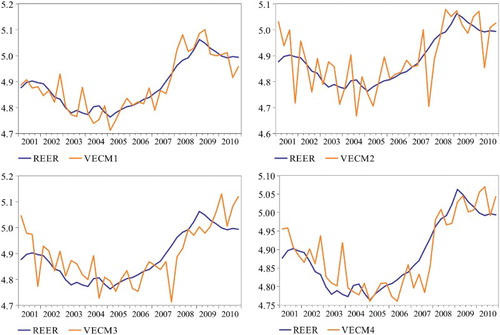
Now we move on to the next stage aimed at assessing the equilibrium real exchange rate of Latvia based on VECM estimates of coefficients in cointegration relationship. First, we apply the estimated coefficients to the actual (non-filtered) values of regressors. The results are presented in Figure 1. The current BEER seems to exhibit larger fluctuations than the REER for all four sets of VECM estimates on account of substantial fluctuations in regressors themselves.

Figure 1. REER and current BEER (2001Q1–2010Q4).

Source: Authors’ estimates. Created with Eviews.

An interpretation of the REER current misalignment based on the current BEER could be misleading because the fundamentals themselves could be far away from equilibrium. To estimate total misalignment, we need a method to obtain potential values of determinants. It can be done by applying a smoothing technique like the Hodrick–Prescott (HP) filter, which has been widely used in the BEER literature to estimate potential values of fundamental variables starting from seminal paper by Clark and MacDonald (1998). But we acknowledge that it provides estimates that are distorted due to asymmetries at the beginning and at the end of the sample. Therefore the long-term BEER estimates for the last four quarters should be treated with caution.

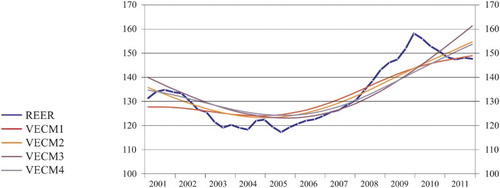
Figure 2 shows the dynamics of the long-term BEER for four estimated models. All four long-term BEER estimates follow broadly similar paths: a somewhat declining BEER until the end-2004 is followed by appreciation. Depreciation observed over 2001–2004 was mainly driven by deteriorating commodity terms of trade and restrictive fiscal policies. The appreciation that followed was brought about by declining openness vis-à-vis trading partners, fiscal expansion, and catch-up in terms of productivity of the tradables sector. There is a clear evidence of overvaluation during the period of unsustainable economic development resulting in double-digit inflation, but its extent and exact timing differ somewhat across the models. Dropping out last four observations, which may suffer from the end-point problem inherent to the HP-filter, we observe that by the end of 2009 the REER was close to its equilibrium level. The magnitude of misalignment was in the range of 0.2–2.9%, suggesting marginal overvaluation. The deceleration in trend real appreciation of equilibrium exchange rate identified by VECM1 for the last four quarters of the sample stems from stabilization in the trend trade-to-GDP ratio, which, however, may just be a reflection of the abovementioned end-point problem.

Figure 2. REER and long-term BEER (2001Q1–2011Q4).

Source: Authors’ estimates. Created with Eviews.

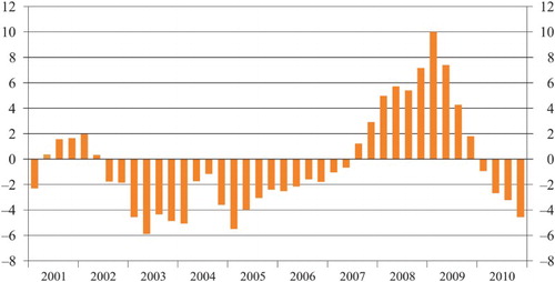
In addition, we have also estimated an arithmetic average of four misalignment measures as stemming from four different VECMs (Figure 3). It suggests that real misalignment reached 10% at the beginning of 2009 but the gap was closed thereafter. An adjustment was attained via internal adjustment strategy implemented by Latvian government as part of the Stabilization Programme of Latvian Economy supported by the IMF/EC and other lenders. Across-the-board cuts in labour costs backed by structural reforms in the public sector have led to real depreciation of the REER and improvement in competitiveness of Latvian economy. The last observation for the fourth quarter of 2010 shows a minor undervaluation of around 4%, which may still suffer from the end-point problem.

Figure 3. Misalignment of Latvia's REER (per cent).

Based on average misalignments stemming from four different VECMs.Source: Authors’ estimates. Created with Eviews.

Policy conclusions from the above results should be drawn with caution. Not only could the above-mentioned end-point problem be an obstacle for laying down straightforward policy conclusions but also caveats regarding the arbitrary choice of statistical filter itself and its parameters could be subject to critique. Setting the value of lambda by applying the HP-filter reflects an agreement regarding the length of the business cycle. In this study we set it equal to the conventional value of 1,600 as suggested by Hodrick and Prescott (1980) for quarterly data. However, this choice is based on the analysis of advanced economies’ (primarily the US) series and an assumption of relatively long cycles that may not be directly applicable for economies in transition. Furthermore, some of the variables used as regressors may not exhibit business cycles whatsoever (Saadi-Sedik & Petri, 2006). By choosing a smaller value of lambda, we would end up in filtered determinants that more closely follow the actual series. That would mean that at any point of time the equilibrium REER is closer to the actual REER, thus reducing the extent of the REER misalignment. Therefore, to make more definitive conclusions, other techniques of the REER misalignment identification could be employed to see whether they point to the same direction.

3.2. The SVAR approach

In this section, we follow Clarida and Gali's (1994) approach and apply the SVAR model to decompose the real exchange rate into permanent and temporary components. We identify long-run structural shocks employing the method by Blanchard and Quah (1989). In particular, Clarida and Gali (1994) construct trivariate SVAR to estimate the relative importance of different types of macroeconomic shocks for changes in relative output (domestic output relative to that of trading partners), relative GDP deflator, and the REER. The long-run triangular identification scheme of Blanchard and Quah is used, in which money or nominal shocks are assumed not to influence the REER and the relative output in the long run, but are likely to raise the price level; supply shocks, in turn, are deemed to affect all three variables in the long run, whereas demand shocks are designed not to affect relative output. Therefore only supply shocks influence relative output in the long run, prices adjust completely to all three shocks, but the REER is affected by both supply and demand shocks. These identifying restrictions are based on the modified version of the Mundell–Fleming–Dornbusch model proposed by Obstfeld (1985). Clarida and Gali (1994) use SVAR estimates for historical decomposition of the REER to extract the contribution of each structural shock to the deviation of the REER from its baseline projection.

The VAR model consists of the first differences of relative output levels, the REER and relative GDP deflators; all variables are in logarithms and calculated relative to Latvia's main trading partners. The VAR system is estimated over the full sample period, namely from the first quarter of 1997 to the third quarter of 2011.

In order to choose an appropriate number of lags in the model, we use a number of lag length criterions. Consistent with the sequential modified likelihood ratio test statistic criteria, we include three lags in the model, which also allows for passing through all residual diagnostic tests (autocorrelation, normality, and heteroskedasticity).

The accumulated impulse responses of the REER, relative output, and GDP deflator to each of the three structural shocks are computed from the estimated VAR coefficients and are presented in Figure 4. As we use relative measures for output and prices, the shocks are thought of as relative supply shocks, relative demand shocks, and relative nominal shocks. All shocks are equal to one standard deviation. To take into account the uncertainty surrounding point estimates of impulse responses, we construct confidence intervals using the Hall's bootstrap percentile confidence interval method (Hall, 1992).

Figure 4. Accumulated impulse responses to shocks.

Source: Authors’ estimates. Created with Eviews.

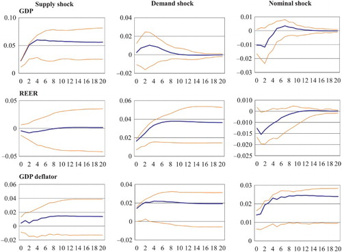
The signs of obtained impulse responses are primarily consistent with theoretical priors. A positive supply shock results in a minor depreciation of the REER in the short run (albeit statistically insignificant) over the first five quarters and then the effect fades. The short-run responses of both output and the REER to one standard deviation supply shock are in line with the theory, because a positive supply shock creates a rise in output; to stimulate the foreign demand for extra output, an improvement in competitiveness is required. It can be achieved by the REER depreciation, but in our study this effect is almost negligible. At the same time, the absence of significant, long-run impact of the supply shock on the REER is not something unique in this paper and resembles the findings of Clarida and Gali (1994), Detken, Dieppe, Henry, Marin, and Smets (2002), and MacDonald and Swagel (2000). The accumulated relative output increases by 6% in the long run. A positive supply shock generates an increase in relative GDP deflator, which, in a way, contradicts the theory. This can be explained by the fact that the theoretical impact of the supply shock rests upon two assumptions: first, it affects all sectors of the economy equally; second, the effect of the supply shock outweighs any derived wealth (demand) effect. The former assumption rules out the possibility of Balassa–Samuelson type effects, which could lead to higher inflation.

The results also show that the responses of relative output, the REER, and relative GDP deflator to the demand shock are positive in the short run. In the long run, the real exchange rate appreciates by 3.6 % and relative GDP deflator increases by 2%. Overall, the signs of impulse responses match our expectations.

As regards the impact of the nominal shock, the relative GDP deflator goes up permanently above the 2% level. The REER depreciates initially, but the effect gradually disappears and the REER returns to its baseline projected value. Output drops by 1% over the first three quarters.

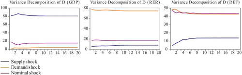
Figure 5 presents the forecast error variance decomposition of variables at different forecast horizons, which can be attributed to each shock in the model. Demand shocks do not explain much of the variance in forecasting the changes in relative output. Only 4% of the variance of forecasting changes in relative output at a 20-quarter horizon is attributed to demand shocks. The demand shock accounts for a substantial fraction of the variance of change in the REER. After 20 quarters, 75% of variation is explained by demand shocks. About 17% of the variance is attributed to nominal shocks. Supply shocks play a very weak role in explaining movements in the REER, accounting for only 8% of the variance at a 20-quarter horizon. Demand and nominal shocks are the main driving forces of this variable, both contributing more than 90% of the forecast error variance. The shocks that cause most of the variation in relative output do not seem to be major contributors to the movements in the real exchange rate. The results are similar to those reported by Detken et al. (2002). At a 20-quarter horizon, the demand and nominal shocks almost equally contribute (about 43%) to the forecast error variance of relative inflation. This result contradicts somewhat Detken et al. (2002), who find that the relative GDP deflator is explained mainly by supply and nominal shocks in the euro area. Unlike the euro area, the demand shock was one of the most important driving forces behind the GDP deflator in Latvia.

Figure 5. Variance decompositions.

Source: Authors’ estimates. Created with Eviews.

The equilibrium real exchange rate can be defined as historical component of the real exchange rate driven by the identified real supply and demand shocks, because these shocks are deemed to influence the REER in the long run. The result is presented in Figure 6 and indicates that the real exchange rate follows very closely the equilibrium. The maximal misalignment over the whole time span is about 4%. The results also indicate that from the fourth quarter of 2008 to the third quarter of 2011, the actual REER was slightly overvalued (maximum overvaluation of 2.4%) if compared with the SVAR-based equilibrium REER. In the third quarter of 2011, the REER and the equilibrium REER were almost equivalent.

Figure 6. REER misalignment according to SVAR approach (per cent).

Source: Authors’ estimates. Created with Eviews.

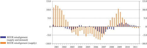
MacDonald and Swagel (2000) suggest that the permanent component of movements in the real exchange rate is solely on account of the contribution by supply shocks, thus stripping out the influence of the demand and nominal shocks. Detken et al. (2002) also exclude the demand-driven shocks by noting that they do not appear to be related to the underlying fundamentals of the economy. In a sense, we can refer to the medium-run exchange rate equilibrium resulting from the contribution of demand and supply shocks, whereas the long-run equilibrium solely depends on the contribution of supply shocks, namely the situation when the impact of demand shock on output dies completely out. Taking into account that a substantial growth in demand in Latvia was caused by credit expansion bringing about rapid appreciation of the REER, we have estimated an alternative measure of misalignment, whereby only the supply shock is supposed to exert impact on the equilibrium REER. According to these estimates, Latvia's REER was clearly overvalued in the period from the fourth quarter of 2007 to the third quarter of 2010, reaching its maximum in the first quarter of 2009; however, similarly to previous results where both shocks were taken into account, the misalignment has already vanished.

Applying SVAR involves both pros and cons. Since the variables employed in SVAR are expressed in first differences rather than in levels the analysis can be conducted without a need to establish a cointegrating relationship between the REER and its determinants. However the identification of shocks in SVAR is not straightforward, since there is no common view in literature which identification scheme is appropriate for SVAR models. Another problem of the SVAR approach is related to the fact that it is not exactly clear if only supply or both supply and (at least partly) demand shocks represent permanent fluctuations in the REER, which in turn may have different policy implications.

4. Structural estimation approaches

4.1. The macroeconomic balance approach

The MB approach estimates the difference between the underlying current account balance projected over the medium term at prevailing exchange rates and an estimated equilibrium current account balance, or ‘CA norm’. The real exchange rate adjustment that would eliminate this difference over the medium term, namely a horizon over which domestic and trading partner output gaps are closed and the lagged effects of past exchange rate changes are fully realized, is then obtained using country-specific elasticities of the current account with respect to the real exchange rate.

The MB approach implies three steps.

1. The underlying current account balance is estimated by correcting the headline balance for the value of domestic output gap and output gaps of trading partners as well as accounting for recent changes in the real exchange rate.

2. An equation linking the current account balance to the set of fundamentals obtains equilibrium current account balance. An equation is estimated using the cross-country panel regression approach; then the equilibrium current account balance is derived based on the estimated coefficients and taking projected values of fundamentals over the medium-term.

3. The required exchange rate adjustment to close the gap between the equilibrium and underlying current account balances is calculated. This step involves the estimation of price elasticities of exports and imports.

Two methodologies are used to estimate the underlying current account balance: the projection-based method and the elasticities-based method. The projection-based method equates the underlying current account with the IMF staff medium-term current account balance projections (the World Economic Outlook [WEO] projection). The elasticities-based method uses elasticities of a reduced-form equation which links the current account balance to domestic and foreign economic activity and the changes in the REER.

The underlying current account balance is therefore obtained by subtracting from the headline current account balance the short-term effect of output gap and recent changes in real exchange rate. This means that the underlying CA balance is estimated under an assumption that both domestic and foreign economies operate at their potential and domestic currency stays at its trend level. The parameters of the reduced-form equation were estimated by Isard and Faruqee (1998, Chapter V) for both industrial countries and developing countries, and these estimates have been widely used by the IMF.

Table 2 shows the estimates of the underlying current account balance of Latvia for 2011 using price elasticities of exports/imports estimated for the panel of both industrial countries and developing economies. The results indicate that the difference between these two estimates is minor, indicating that the current account of Latvia recorded a small deficit when accounting for temporary factors. At the same time the value of the underlying current account balance is quite sensitive to the estimates of domestic and foreign output gaps, which are widely known to be quite uncertain. European Commission estimates assume that the output gap of Latvia was −4.3% of GDP in 2011 (EC, 2012). However, the potential output estimates are subject to frequent revisions especially in light of unexpected changes in economic activity. One percentage point of GDP revision in the level of output gap for 2011 would yield a change in the underlying current account balance by 0.9% point of GDP.

Table 2. The underlying current account balance of Latvia in 2011.

		Price elasticities for industrial countries	Price elasticities for developing countries
Headline CA balance	1	–1.2	–1.2
Latvia's output gap	2	–4.3	–4.3
Latvia's imports (% of GDP)	3	0.63	0.63
Coefficient	4	1.5	1.5
Impact of Latvia's output gap	5 = 2 × 3 × 4	–4.1	–4.1
Trading partners’ output gap	6	–1.5	–1.5
Latvia's exports (% of GDP)	7	0.59	0.59
coefficient	8	1.5	1.5
Impact of output gaps in trading partners	9 = 6 × 7 × 8	–1.4	–1.4
Lagged effects of past changes in competitiveness	10	–0.5	–0.3
Adjustment for temporary factors	11 = 5 – 9 – 10	–2.2	–2.4
Underlying CA balance	12 = 1 + 11	–3.5	–3.6

Sources: Authors’ calculations, European Commission (2012), Eurostat and Isard and Faruqee (1998, Chapter V).

As mentioned above, the equilibrium level of the current account balance is derived on the basis of estimated coefficients of the cross-section panel regression and taking projected values of fundamentals over the medium term.

The relationship between the current account balance and its fundamental determinants has been estimated by Lee et al. (2008) for a large set of industrial and developing countries over 1973–2004 using the pooled ordinary least squares regression. The regression coefficients may not be directly applicable to Latvia due to the fact that Latvia is not included in the country sample. However, when estimating the equilibrium exchange rate the IMF uses these coefficients for the assessment of equilibrium current account balance. The regression includes the following variables: budget balance, old-age dependency ratio, population growth, output growth, net foreign assets, oil balance, and relative income. The former four variables are calculated vis-à-vis those of trading partners.

The values of the budget balance, oil balance, and output growth forecast for 2017 are taken from the IMF WEO (2012), whereas the forecasts of old-age dependency ratio, population growth, and initial foreign assets (per cent of GDP) are taken from the Eurostat. According to the IMF WEO (2012), in 2017 Latvia's output growth is expected to be 4%, the budget balance ratio 0.4% of GDP, and oil balance −6.1%, and the relative income of Latvia was by 67.% lower than that of the USA in 2011. The old age dependency ratio is calculated as a ratio of the population above 65 to the population between 30 and 64, using the Eurostat EUROPOP2010 forecast for 2015, and is equal to −0.5% in Latvia in 2015. The population growth is calculated as an average growth rate based on the Eurostat EUROPOP2010 forecast for 2010 and 2015. The ratio of foreign assets in 2011 in Latvia was −72.5% of GDP. To increase the robustness of equilibrium current account balance estimates, we apply three different sets of coefficients: coefficients estimated by Lee et al. (2008) using pooled and hybrid pooled regressions, and those estimated by Rahman (2008) for a panel of both industrial and developing countries, including Latvia. In addition to variables described above, Rahman (2008) includes an index capturing the effect of investment climate, which is constructed using the average of the European Bank for Reconstruction and Development transition indicators in such areas as large scale privatization, small scale privatization, governance and enterprise restructuring, price liberalization, trade and foreign exchange system, and competition policy. Rahman (2008) shows that the transition indicator exhibits a strong negative correlation with the CA balance.

Coefficient estimates, medium-term values of fundamentals applied to these estimates and estimates of equilibrium current account balance of Latvia are shown in Table 3. The results suggest that the equilibrium current account balance for Latvia is in the range of −3.3 to −5.8% of GDP. These estimates imply that the underlying current account balance is either close to or larger than the equilibrium level of current account, meaning that the REER is close to its equilibrium (or even somewhat undervalued).

Table 3. The medium term equilibrium current account balance of Latvia.

		Coefficients			Contribution (%)
Regressors	Value (%)	Lee et al.: pooled estimation	Lee et al.: hybrid pooled estimation	Rahman: pooled estimation	Lee et al.: pooled estimation	Lee et al.: hybrid pooled estimation	Rahman: pooled estimation
Budget balance	–0.9	0.20	0.19	0.22	0.2	0.2	0.2
Old-age dependency	–2.4	–0.14	–0.12	–0.04	0.3	0.3	0.1
Population growth	–0.6	–1.21	–1.03	–0.63	0.7	0.6	0.4
Initial foreign assets (% of GDP)	–72.5	0.02	–	0.03	–1.4	–	–2.2
Lagged current account balance	–5.0	–	0.37	–	–	–1.9	–
Oil balance	–6.1	0.23	0.17	0.44	–1.4	–1.0	–2.7
Output growth	1.5	–0.21	–0.16	–0.18	–0.3	–0.2	–0.3
Relative income	–67.6	0.02	0.02	–0.01	–1.4	–1.4	0.7
Investment climate	400.0	–	`	–0.01	–	–	–4.0
Constant	100.0	0.00	0.00	0.02	0.00	0.00	2.0
Equilibrium current account	–	–	–	–	–3.3	–3.4	–5.8

Sources: Authors’ calculations, Lee et al. (2008), Rahman (2008), Eurostat and International Monetary Fund (2012).

The real exchange rate gap, namely the gap between the current value of REER and the equilibrium REER needed to bring the current account balance to its equilibrium level, is calculated using the value of price elasticity of exports and imports:(6)

The extent of misalignment is shown in Table 4 under different assumptions regarding price elasticities and the equilibrium current account. The elasticity of the current account balance ratio to GDP with respect to the REER is calculated to be −0.37 if price elasticities of industrial economies are used, and much smaller, −0.14, if elasticities of developing economies are explored. Under all mentioned assumptions, the REER is close to its equilibrium or estimated to be somewhat undervalued when the coefficients estimated by Rahman (2008) are used. The estimates of REER misalignment shown in the last column of Table 4 implying huge undervaluation of the REER seem implausible owing to the fact that the current account balance elasticity is close to zero, making an estimate of the REER misalignment extremely sensitive to any deviation in the current account balance.

Table 4. Real exchange rate misalignment in 2011 according to MB approach.

	Price elasticities for industrial countries			Elasticities for developing countries
	Lee et al.: pooled estimation	Lee et al.: hybrid pooled estimation	Rahman: pooled estimation	Lee et al.: pooled estimation	Lee et al.: hybrid pooled estimation	Rahman: pooled estimation
Underlying CA balance	–3.5	–3.5	–3.5	–3.6	–3.6	–3.6
CA norm	–3.3	–3.4	–5.8	–3.3	–3.4	–5.8
CA misalignment	–0.2	0.0	2.3	–0.28	–0.15	2.2
Elasticity	–0.37	–0.37	–0.37	–0.14	–0.14	–0.14
RER misalignment	0.5	0.1	–6.2	2.1	–1.1	–16.2

Sources: Authors’ calculations and Isard and Faruqee (1998).

The most obvious advantage of the MB approach is that it could be easily applied to any country, even one that does not have long series of macroeconomic variables to estimate the current account regression or has not been included in the panel estimation implemented by Lee et al. (2008) or similar studies.

There are also a number of drawbacks of this approach:

1. The equilibrium current account estimates under the MB approach are very sensitive to coefficients used. Unfortunately, the IMF study (Lee et al. (2008)) does not report standard deviations of the estimated coefficients, thus we are not able to conduct a meaningful sensitivity exercise. However, the study by Bussière et al. (2010) by running 16,384 different regressions shows that the range of coefficient estimates is actually very broad.

2. Medium-term values of regressors are proxied by the WEO projections for the last year available. However, there are some reasons to believe that even medium-term projected values could deviate from the steady state.

3. It should be noted that coefficients on both the CA norm and price elasticities of exports and imports estimated for a panel of countries which does not include Latvia may not be directly applicable when assessing the equilibrium REER of Latvia.

4. The underlying current account balance is sensitive to the estimate of the output gap. As mentioned earlier, a 1% point of GDP change in the level of output gap would yield a change in the underlying current account balance of Latvia by 0.9% point of GDP that would modify the estimates of the REER misalignment by 2.6–7.0% points.

4.2. The ES approach

Similar to the MB approach, the ES approach is a method of calculation of real exchange rate which is consistent with the medium-term macroeconomic equilibrium, but this medium-term equilibrium is calculated in a different way. To some extent, this approach is similar to the public debt sustainability analysis where budget deficit consistent with some steady state public debt ratio is determined. Here, in contrast, the level of current account balance stabilizing the net foreign assets (NFA) at a given level is estimated by applying the accumulation equation for NFA. The equation states that changes in NFA are due either to net financial flows or changes in the valuation of outstanding foreign assets and liabilities. Assuming zero capital gains, the CA norm (ca^s) that would be compatible with some steady state level of NFA (bs) is given by(7) where g is the growth rate of real GDP, π is the inflation rate, whereas b^s and ca^s are NFA and CA as shares of GDP, respectively.

Applying WEO (April 2012) forecasts for Latvia, where g = 4.0% and π = 2.1% in 2017, and assuming that the NFA remains unchanged, namely b^s = −72% (the figure reflects position in 2011, which is in line with the CGER methodology, and is calculated using Eurostat data), yields the CA norm ca^s = −4.2%. If we assume that the current NFA stock is unsustainable per se and use more conservative assumptions on equilibrium NFA stock, namely b^s = −50% or −35%, the CA norm increases to −2.9% and −2.0% accordingly. Following these assumptions, the extent of misalignment is calculated to be in the range from −1.9% to +3.9%, as shown in Table 5.

Table 5. Real exchange rate misalignment in 2011 according to ES approach.

	Three scenarios according to different assumptions on benchmark level of NFA
Growth rate of real GDP	0.04	0.04	0.04
Inflation rate	0.02	0.02	0.02
Benchmark level of NFA (%)	–72	–50	–35
Equilibrium CA (%)	–4.2	–2.9	–2.0
Underlying CA balance in 2011 (%)	–3.5	–3.5	–3.5
CA balance misalignment (%)	0.7	–0.6	–1.4
Elasticity	–0.37	–0.37	–0.37
RER misalignment (%)	–1.9	1.6	3.9

Sources: Authors’ calculations, Eurostat, Isard, and Faruqee (1998, Chapter V) and International Monetary Fund (2012).

In contrast to the MB approach, the ES approach is stock equilibrium consistent, as it explicitly aims at reaching and sustaining a certain benchmark level of NFA. The ES approach is simple and quite straightforward to use; therefore, similar to the MB approach, it could easily be applied to any country, including that lacking long macroeconomic series. However equilibrium current account estimates are very sensitive to assumptions regarding the rates of GDP growth and inflation, as well as to the assumed benchmark level of NFA. The above discussed caveat of using output gaps in determining underlying current account balance, as well as regarding the price elasticity of exports and imports applies to the ES approach too.

4.3. The NATREX approach

In this section, we consider the NATREX approach introduced and developed by Stein in a series of papers and books (1994, 1997, 1999, 2006), which is regarded to be a model with strong theoretical micro-founded structure. It links the developments in the REER to the developments in the factors explaining investment, consumption, and trade balance behaviour. These factors, in turn, are derived by optimizing agents’ decision-making. The model is stock-flow consistent and explicitly distinguishes between the medium-term NATREX and the long-term NATREX.

The medium-term NATREX is characterized by internal equilibrium (namely there are no deflationary/inflationary pressures in the economy) and external equilibrium (the real interest rate is equal to the world's real interest rate), and capital stock and net foreign assets/debt are exogenous. In the long-term NATREX, capital stock and net foreign assets/debt reach their steady state level, namely are assumed to be endogenous. In this model, there are decisions on how much to invest (by maximizing firm profits) and how much to spend and save correspondingly (by optimizing consumers’ intertemporal utility). By optimizing economic agents’ decisions on consumption, production, and investment, one can derive behavioural equations consistent with the internal–external balance. Following Detken et al. (2002) who used this approach to estimate the equilibrium exchange rate of euro, we estimate the following behavioural equations in linear form:(8) (9) (10) where C is aggregate consumption (private and public), K is capital stock at constant prices, Y is GDP at current prices, Y_r is GDP at constant prices, F is net foreign debt, I is investment (public and private), P_r denotes marginal product of capital and is measured as a capital share in the production function times output over capital ratio, i_L is long-term interest rates, R is the REER, TB denotes trade balance, A denotes total economy's absorption (investment plus consumption), and, finally, * is the notation for foreign consumption to GDP ratio.

In addition to the three behavioural relationships, the following national account identity is specified:(11) where SCN denotes variation in debt stocks. The current account is divided into two components, namely the trade balance and residual component.

The long-term NATREX can be obtained under an assumption that capital stock and net foreign debt reach their steady state levels. These, in turn, stem from stock accumulation rules and can be represented by the following relationships:(12) (13) where the parameter δ is the depreciation rate of capital stock per quarter, q is nominal GDP growth rate, g is real GDP growth rate, P_Y is GDP deflator, and P_I is gross fixed capital formation deflator. Noteworthy, Equation (12) is just another representation of Equation (7).

We use the following approach to estimate the medium-term NATREX. First, we identify the order of integration of variables under consideration. Second, we estimate three behavioural Equations (8)–(10) using VECMs and test for the presence of cointegrating vectors using the Johansen cointegration test. Third, by using the national account identity (11), estimated coefficients of cointegrating vectors and medium-term values of variables, we estimate the medium-term NATREX.

We use the data for the period between the first quarter of 2001 and the third quarter of 2011 in the estimation. All considered variables are integrated of order 1.⁴

To estimate the vector error correction model, we make use of the Johansen cointegration approach. We identify cointegrating vectors for the consumption ratio (1), investment ratio (2) and trade balance ratio, (3) with theoretically plausible signs, except for the sign of the impact of net marginal product of capital⁵ on investment. The cointegrating parameters, their t-values, adjustment coefficients, and the results of diagnostic tests of three VECMs are reported in Table 6. In all estimated VECMs, we have found one cointegrating vector. The adjustment coefficients for endogenous variables are significant at the 5% level, except for the error correction term for the trade balance. The gap between the actual and equilibrium trade balance ratio is not closed by adjustment in the trade balance itself, and it returns to its equilibrium by adjustment in domestic absorption and/or foreign consumption. It should be also noted that the REER has a negative impact on investment and trade balance where the negative impact of REER appreciation is higher on the former than on the latter.

Table 6. Estimations of VECMs for behavioural equations^a.

	Variable	Consumption function	Investment function	Trade balance function
	Constant	86.822	401.625	93.142
Long-run parameters	Capital ratio	0.037 (2.055)	–	–
	Net foreign debt	–0.185 (–5.529)	–	–
	MPK minus interest rate	–	–4.577 (–3.971)	–
	Real exchange rate	–	–2.528 (–4.945)	–0.231 (–3.759)
	Absorption	–	–	–1.651 (–9.367)
	Foreign consumption	–	–	1.341 (2.325)
Adjustment coefficients	Consumption	–0.607 (–4.347)	–	–
	Investment	–	–0.068 (–4.597)	–
	Trade balance	–	–	0.126 (0.752)
Diagnostic tests	Serial correlation test	12.781 [0.173]	13.509 [0.141]	17.360 [0.363]
	Normality test	37.080 [0.057]	11.771 [0.988]	49.078 [0.699]
	Heteroskedasticity test	58.914 [0.720]	58.693 [0.139]	183.280 [0.418]

Source: Authors’ estimates.

^aNote: t-statistic values for long-run parameters and adjustment coefficients are provided in parenthesis, probability levels for the diagnostic tests are reflected in square brackets.

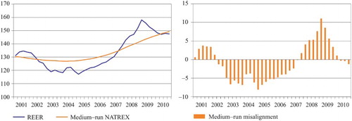
As has already been mentioned, to obtain the medium-run NATREX one should insert cointegration relationships [8]–[10] into identity [11] and express the real exchange rate R as a function of exogenous regressors. Then cyclical components of variation in debt stocks , net marginal product (Pr–i_L), and foreign consumption ratio should be removed using the HP filter. The medium-term NATREX is estimated on the basis of the actual values of capital stock and net foreign debt. Figure 7 presents the medium-run NATREX together with medium-run misalignment. It shows that the actual real exchange rate had converged to its medium-run NATREX by the second quarter of 2010. The REER seems to have been undervalued over the period from the third quarter of 2002 to the third quarter of 2007, followed by a period of overvaluation from the fourth quarter of 2007 to the first quarter of 2010. During the time span from the first quarter of 2001 to the fourth quarter of 2004, the medium-run NATREX was broadly stable. After 2004, it showed a clear upward path. The major contributing factor to the appreciation of the medium-run NATREX was the fall in net return on capital. At the same time, only a minor part of the medium-run NATREX evolution is explained by the behaviour of capital stock, stock of net foreign debt, and foreign consumption ratio.

Figure 7. REER, medium-run NATREX and medium-run misalignment.

Source: Authors’ estimates. Created with Eviews.

To obtain the long-run NATREX in addition to solving the system of Equations (8)–(11), one should assume that capital stock and net foreign debt have reached their steady state levels, as represented by Equations (12) and (13). These steady state levels are derived from the dynamic equations of capital and net foreign debt accumulation. Following Detken et al. (2002), the equation for steady state stock of net foreign debt is derived assuming that the net factor income ratio to GDP is exogenous.

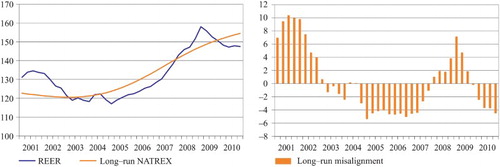
The REER and the long-run NATREX are depicted in Figure 8. The long-run NATREX shows a similar pattern if compared to the medium-term NATREX with larger deviations from the actual REER and bigger misalignment at the beginning of the sample, and smaller misalignment thereafter, including the period of pre-crisis overvaluation of Latvian REER. Nevertheless, it points to a similar path of misalignment over the period under consideration with the period of initial overvaluation (from the first quarter of 2001 to the first quarter of 2003), undervaluation in the middle of the first decade of the 2000s (from the fourth quarter of 2004 to the third quarter of 2007), and overvaluation of the pre-crisis and early crisis period (from the first quarter of 2008 to the third quarter of 2009).

Figure 8. REER, long-run NATREX and long-run misalignment.

Source: Authors’ estimates. Created with Eviews.

The main strength of the NATREX is related to the fact that it is a micro founded approach, implying it is derived from optimizing economic agents’ behaviour. Furthermore it is stock-flow consistent approach. However the critique of smoothing technique choice discussed in Section 3.1 applies to the NATREX as well, since cyclical components of regressors are being removed using the HP filter with all of the implications considered in Section 3.1. Besides that, one should take into consideration high sensitivity of the long-run NATREX estimates to the assumed steady state rate of real and nominal GDP growth and the rate of capital depreciation. Therefore the long-term NATREX estimates should be interpreted with considerable caution.

5. Comparison of estimates

Finally, we compare the results of four estimates that assess the dynamics of misalignment obtained by using three different approaches: the average of the long-term BEER estimates, the medium and the long-term NATREX, and SVAR driven by supply shocks. We also refer to the two point estimates of misalignment obtained by the MB and the ES approaches. All four estimates that assess the dynamics of misalignment point to a pretty similar path of misalignment despite the fact that all three methodologies differ significantly in terms of theoretical background and macroeconomic time series used. All four estimates of misalignment pointed to the peak overvaluation in the first quarter of 2009 and a subsequent adjustment towards equilibrium (Figure 9). Differences arise with regard to the timing of switching from overvaluation to undervaluation and their extent. The highest swings measured by standard deviation are shown by the SVAR estimates of misalignment. This stems from the fact that the SVAR misalignment is measured with respect to the supply-shock-generated equilibrium REER, which does not exhibit significant fluctuations. The smallest swings occur in the long-term BEER misalignment. This, in turn, is the result of estimating the long-term BEER directly from the reduced-form equation. If we look at the pairwise correlations between different estimates of the REER misalignment during 2001–2010, we can conclude that the estimates are indeed highly correlated. The highest correlation is observed between the long-run BEER and the medium-term NATREX, and between the SVAR and the long-run NATREX. As regards the latter two, both are of a long-run nature indeed, as demand shocks die out only after a considerable lapse of time, and the convergence of capital stock and net foreign debt to their long-run steady state values can be accomplished over a long time span as well (Table 7).

Figure 9. REER misalignment by four approaches.

Source: Authors’ estimates. Created with Eviews.

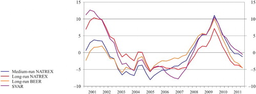
Table 7. Pairwise correlation between different misalignment estimates.

	Medium-run NATREX	Long-run NATREX	Long-run BEER	SVAR
Medium-run NATREX	1.00	0.66	0.92	0.84
Long-run NATREX	0.66	1.00	0.52	0.91
Long-run BEER	0.92	0.52	1.00	0.65
SVAR	0.84	0.91	0.65	1.00

Source: Authors’ estimates.

Referring to point estimates of misalignment derived by the MB and the ES approaches, both point to closeness of the REER to its equilibrium level in 2011 that fits rather well into the overall picture. The MB approach using different estimates of equilibrium current account and price elasticities for industrial countries displays the misalignment in the range of +0.5% to −6.5%, a result apparently rather consistent with the outcomes derived by the three above-mentioned approaches at the end of the sample period, that is, the end of 2010. Also, the misalignment derived by the ES approach using the current level of NFA as a benchmark (−1.9%) fits well into this range, and only more conservative assumptions on equilibrium NFA level produced a small positive misalignment of up to +3.9%.

6. Conclusions

The purpose of this study was to estimate the equilibrium REER of Latvia, using different methodologies. Given that equilibrium exchange rate estimates are subject to substantial uncertainty and are sensitive to different assumptions, it is important to employ a broad set of approaches that differ in terms of the underlying theoretical background and macroeconomic time series before any definitive conclusions on the REER misalignment are made. In the study we make use of both structural approaches and direct estimation approaches with some of the structural approaches being flow equilibrium consistent and some stock consistent. As no one method could be regarded as superior and as each of them has its own strengths and weaknesses discussed in this study one cannot rely on just one approach; therefore one should use a variety of methods to assess the equilibrium position of a country`s REER to increase the credibility of results.

According to the BEER approach, Latvia's REER was found to be almost in equilibrium at the end of 2009 and slightly undervalued after the downward adjustment from the overvalued level before the recent crisis. It should be taken into account that the estimates of the long-term BEER for the last four quarters of the sample should be interpreted with caution, as they suffer from the end-point problem inherent to the HP filter. According to SVAR, the gap between the supply-driven equilibrium REER and the actual REER has also been closed shortly after the period of currency overvaluation prior to the recent recession.

Our estimates derived from both the macroeconomic balance and the ES approach show that Latvia's REER was overall close to its equilibrium in 2011. Depending on different specifications used, small misalignments on both ends (under-evaluation and overvaluation) were derived. At the same time, these results are rather sensitive to the assumptions and coefficients used. Both the medium-run and the long-run NATREXs indicate that there has been an overvaluation of Latvia's REER during the pre-crisis period, but the gap has disappeared thereafter. However, the long-run NATREX estimates are highly sensitive to assumptions regarding the GDP growth, inflation, and depreciation rate and therefore should be interpreted with caution.

All in all, the results of all approaches used in this study indicate that Latvia's REER does not appear to be significantly misaligned at the current juncture, and the real exchange rate of Latvia, after the appreciation during boom years and the subsequent adjustment, remains close to its equilibrium level.

Disclosure statement

No potential conflict of interest was reported by the authors.

Notes

1. However, recently a group within the IMF was established aimed at developing an alternative methodology for assessing current accounts and exchange rates in a multilaterally consistent framework. The pilot version of the External Balance Assessment methodology was first presented in 2012 and has since been under discussion both within the IMF and with other international organizations.

2. Unit root tests results are available upon request.

3. available upon request.

4. Unit root tests are available upon request.

5. We refer to net marginal product of capital as a differential between marginal product of capital and nominal interest rate.

References

- Blanchard, O., & Quah, D. (1989). The dynamic effects of aggregate demand and supply disturbances. American Economic Review, 79(4), 655–673.
- Bussière, M., Ca’ Zorzi, M., Chudik, A., & Dieppe, A. (2010). Methodological advances in the assessment of equilibrium exchange rates (ECB Working Paper No. 1151). Frankfurt am Main: ECB.
- Clarida, R., & Gali, J. (1994). Sources of real exchange rate fluctuations: How important are nominal shocks? (NBER Working Paper No. 4658). Cambridge: NBER.
- Clark, P. B., & MacDonald, R. (1998). Exchange rates and economic fundamentals: A methodological comparison of BEERs and FEERs (IMF Working Paper No. 67). Washington, DC: IMF.
- Detken, C., Dieppe, A., Henry, J., Marin, C., & Smets, F. (2002). Model uncertainty and the equilibrium value of the real effective euro exchange rate (ECB Working Paper No. 160). Frankfurt am Main: ECB.
- European Commission. (2012). Cyclical adjustment of budget balances. Brussels: Author.
- Hall, P. (1992). The bootstrap and edgeworth expansion (Springer series in statistics). New York, NY: Springer-Verlag.
- Hodrick, R., & Prescott, E. (1980). Postwar U.S. business cycles: An empirical investigation. (Carnegie Mellon University Discussion Paper No. 451). Reprinted in an updated version as ‘Postwar U.S. business cycles: An empirical investigation’, Journal of Money, Credit and Banking, 1997, 29(1), 1–16.
- International Monetary Fund. (2006). Methodology for CGER exchange rate assessments. Washington, DC: Author.
- International Monetary Fund. (2012). World Economic Outlook database. Washington, DC: Author.
- Isard, P., & Faruqee, H. (1998). Exchange rate assessment: Extensions of the macroeconomic balance approach (IMF Occasional Paper No. 167). Washington, DC: IMF.
- Lee, J., Milesi-Feretti, G. M., Ostry, J. D., Prati, A., & Ricci, L. A. (2008). Exchange rate assessments: CGER methodologies (IMF Occasional Paper No. 261). Washington, DC: IMF.
- MacDonald, R., & Swagel, P. (2000). ‘Business cycle influences on exchange rates: Survey and evidence’ in IMF World Economic Outlook Supporting Studies. Washington, DC: IMF.
- Obstfeld, M. (1985). Floating exchange rates: Experience and prospects. Brooking Papers on Economic Activity, 2, 369–450.
- Rahman, J. (2008). Current account developments in New Member States of the European Union: Equilibrium, excess and EU-phoria (IMF Working Paper No. 92). Washington, DC: IMF.
- Saadi–Sedik, T., & Petri, M. (2006). To smooth or not to smooth – the impact of grants and remittances on the equilibrium real exchange rate in Jordan (IMF Working Paper No. 257). Washington, DC: IMF.
- Stein, J. L. (1994). The natural real exchange rate of the United States Dollar and determinants of capital flows. In J. Williamson (Ed.), Estimating equilibrium exchange rates (pp. 133–176). Washington, DC: Institute for International Economics.
- Stein, J. L. (1997). The equilibrium real exchange rate of Germany. In J. L. Stein, & P. R. Allen, (Eds.), Fundamental determinants of exchange rates (pp. 182–224). New York, NY: Oxford University Press.
- Stein, J. L. (1999). The evolution of the real value of the US Dollar relative to the G7 currencies. In R. MacDonald, & J. L. Stein (Eds.), Equilibrium exchange rates (pp. 67–101). Dordrecht: Kluwer Academic.
- Stein, J. L. (2006). Stochastic optimal control, international finance, and debt crises. New York, NY: Oxford University Press.
- Syllignakis, M. N., & Kouretas, G. P. (2011). Markov-Switching regimes and the monetary model of exchange rate determination: Evidence from the Central and Eastern European markets. Journal of International Financial Markets, Institutions and Money, 21(5), 707–723. doi: 10.1016/j.intfin.2011.04.005
- Williamson, J. (1983). The exchange rate system. Washington, DC: Institute for International economics.