Macroeconomic volatility, monetary union, and external exposure: evidence from five Eurozone members

ABSTRACT

Membership in a common currency area is thought to promote economic stability by facilitating macroeconomic convergence, but a country might give up important monetary policy tools that could help stabilize its economy following a shock. The effect of a common currency on macroeconomic volatility can therefore be ambiguous. This study examines five Central and Eastern European countries that joined the Eurozone since 2005; their differences, particularly with regard to the countries’ economic performance and pre-accession exchange-rate regimes, help drive a unique set of results. Structural breaks in the volatility of real output, consumption, and investment generally correspond to events other than Eurozone accession, and Vector Autoregressive methods show that global shocks have more of an impact on output volatility than do regional shocks or economic openness. Spillovers affect Latvia and Lithuania more than Estonia, Slovakia, or Slovenia, which suggests that a unified currency space might have difficulty managing idiosyncratic shocks.

JEL Classification:

• F45

Keywords:

• Macroeconomic Volatility
• Structural Breaks
• Eurozone
• Central and Eastern Europe

1. Introduction

For the formerly planned economies of Central and Eastern Europe (CEE), membership in the European Union had long offered the promise of re-integration with the West. Unified markets for goods and services, as well as for labour and capital, could help bring economic growth and stability similar to that enjoyed by more established members of the EU. Small open economies can enjoy seamless trade integration and stable export and import prices with many of their largest trade partners, as well as to “import” credibility and stability, often leading to increased investment flows and lower inflation. De Grauwe and Schnabl (2005) outline many of these benefits, but also note the specific challenges faced by CEE countries in joining the Euro.

Of the 11 CEE countries in the EU, only Slovakia, Slovenia, and the Baltic countries of Estonia, Latvia, and Lithuania have adopted the Euro by 2020. Perhaps not coincidentally, all five were members of multinational states during the Soviet period. At the same time, neighbours such as the Czech Republic and Poland maintain independent currencies and have not offered any serious plans to join the Eurozone. Since the Baltics had adopted euro-backed currency boards long before they formally joined the currency union, membership itself might not have brought many drastic changes compared to Slovakia, Slovenia, or any future Eurozone members.

One major drawback of joining a common currency is the complete loss of monetary policy as a tool to smooth macroeconomic fluctuations. Faced with large expansions or contractions in economic activity, such a country would be forced to use fiscal policy, or allow for international labour flows, to help tame its business cycle. Latvia, for example, implemented a controversial ‘internal devaluation’ in the aftermath of the 2009 global financial crisis, which allowed the country to simultaneously restore competitiveness and maintain its euro peg so that its candidate status would not be jeopardized. The country also lost a quarter of its population through emigration.

These two competing concepts – a common currency as a path toward increased stability, as well as a channel for increased macroeconomic fluctuations – therefore conflict, which motivates the current study. But, since Latvia faced policy constraints under its (quasi-) currency board arrangement before it joined the euro, it is possible that these competing pressures might not manifest themselves specifically at the time of accession. Significant events may be related to macroeconomic, political, and other factors.

Each economy has had a different experience in terms of the timing of Eurozone accession, so results for the five countries examined here might differ in ways that go beyond individual country characteristics. Figure 1 depicts their Hodrick-Prescott filtered business cycles and log real GDP, and shows how each country acceded to the common currency at a different phase of expansion or contraction. Slovenia, which joined first, did so during the pre-crisis boom, while Slovakia joined right at the beginning of the post-crisis recovery. In the Baltics, Estonia acceded during the middle of the recovery, while Latvia and Lithuania did so during a mild downturn that followed mid-decade.

Figure 1. Output Cycles and Euro Accession, 1995–2018. Black line = Hodrick-Prescott filtered log real output; grey line = unfiltered values (scaled to cycle range). Black dashed line = Euro accession; grey dashed line = ERM-II membership (Slovakia and Slovenia)

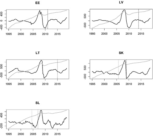
As noted above, the Baltics followed different exchange-rate regimes than did the other two countries. When they joined the European Exchange Rate Mechanism (ERM-II) in 2004, Estonia, Lithuania, and Latvia had already been fixed to the German Mark, U.S. dollar, and the IMF's SDR, respectively. As noted by Bauer and Herz (2005), Slovenia and Slovakia had more freely floating currencies and joined the ERM-II in late June 2004 and late November 2005, respectively.¹ Joining the euro, therefore, might not have led to a clean ‘break.’

In addition to the business cycle and in the exchange-rate regime, other macroeconomic conditions such as economic size and openness allow for the absorption and transmission of shocks. These small open economies have been subject to volatile capital inflows and instability elsewhere in Europe. In particular, the capital flow ‘bonanza’ in the run-up to the 2008 financial crisis was particularly destabilizing. Following the ‘sudden stop’ that followed, it took countries in the region years to recover.

Other differences might help explain differences among these countries’ volatility processes and susceptibility to shocks as well. Differences in the speed and boldness of economic reforms, tax and social welfare systems, and geographic and political orientation may also play a role. Firdmuc (2003) discusses the positive connections between political and economic liberalization throughout the region, and Staehr (2017) describes a number of unique political and economic features that define the Baltic countries, for example. While the Baltics and Central Europe have performed much better than many counterparts to the South and East, there are still differences that might help drive further research.

This study makes three key contributions to the literature. Its primary two areas of focus are to estimate the time-varying macroeconomic volatility for a set of CEE euro members and assess its time-series properties with regards to structural changes that might be connected to changes in currency policy. Additionally, it tests for the possibility of asymmetric shocks for the different countries in the region. The study does so as follows. First, it calculates quarterly time series of output, consumption, and investment volatility for five CEE countries from 1995 to 2018, comparing a set of alternative measures and choosing one to use in further analysis. Second, it tests for structural breaks in each series, examining whether the date of Eurozone accession corresponds to such a break, or whether other factors might be more influential. The study also compares average volatility in both the pre- and post-euro periods, as well as in the break-defined subperiods. Finally, the relative impact of external volatility, as well as economic openness as a transmission channel, are examined empirically using Vector Autoregressive (VAR) methods. Regional differences are found that might pose policy challenges; of the economies in this study, the Baltic countries of Latvia and Lithuania are most affected by trade openness and external shocks that originate both globally and within the EU itself.

2. Previous studies related to macroeconomic volatility and economic integration

The idea that a common currency such as the Euro might limit macroeconomic adjustment dates back at least to Mundell (1961), whose Optimal Currency Area theory predicted the challenges that states would face as a result. Without an independent monetary policy, alternative adjustment mechanisms such as migration and fiscal transfers would emerge as a means to deal with asymmetric area-wide shocks. Only highly integrated economies, with similar business cycles, would, therefore, benefit from a common currency.

A large share of previous studies tends to focus on business-cycle synchronization as a method of assessing regional economic fluctuations, rather than on the volatility processes themselves. These studies often find surprisingly limited, or even negative, changes in comovements following the introduction of a common currency. Barro and Tenreyro (2007) find decreased comovements in output shocks, and Lehwald (2013) concludes that synchronization has decreased for peripheral EU countries as opposed to the core. Miles and Vijverberg (2018) also show limited integration in their analysis of quarterly industrial production from 1983 to 2009; only one of eight countries exhibited increased synchronization after the euro came into existence. Campos et al. (2019), in their meta-analysis of studies of business cycle synchronization, find that four of the five countries examined in the current study (all but Slovenia) show no increase in this type of integration.

Until the 2008 crisis, macroeconomic volatility was often considered to have been successfully reduced through adept fiscal, and particularly monetary, policy. Avouyi-Dovi and Sahuc (2016), for example, find that Eurozone volatility was reduced after 1994, well before the euro. Likewise, Enders et al. (2013) find that business cycle cross-correlations increased, but that macroeconomic volatility was ‘largely unchanged,’ after the euro was introduced. Nevertheless, Beetsma and Giuliodori (2010) show that monetary union can strengthen fiscal spillovers, and Gradzewicza and Makarskia (2013) predicted an increase in output and consumption volatility were Poland to join the Eurozone. Because variability has by no means been completely smoothed away, macroeconomic volatility continues to be worthy of investigation.

Of the major GDP components, consumption is generally given the most attention. Stability is beneficial to households’ well-being, and international financial markets allow them to ‘smooth’ away excess consumption fluctuations through lending or borrowing. Output volatility is studied more than investment, which, because of businesses’ reaction to uncertainty, usually varies significantly. The current study focuses on all three types of volatility equally, uncovering differing results across variables as well as countries.

Much of the literature on the relationship between economic integration and macroeconomic volatility focuses on three key channels. Most often examined is the role of financial openness, which serves as both a transmission channel for foreign shocks and as a method of smoothing away fluctuations. The second, trade openness, works primarily through real channels as one country's output shock will affect its imports, and therefore its partners’ exports and GDP. Third, external shocks have the potential to spill over to a country's economy directly. In particular, a major regional trade partner's degree of risk, or increased variability in the prices of global commodities, could lead to increased macroeconomic instability for an open economy. Volatility in commodity prices can also affect a country's export revenue, import costs, and producer profits.

Important studies of the impact of increased financial linkages include a review by Kose et al. (2009), who note that many previous empirical analyses had provided mixed results. Buch and Yener (2010) find that while consumption volatility had been reduced by increased financial openness in the G-7 countries, the decrease was not large relative to output volatility. Meller (2013) finds that financial integration has a negative effect on output volatility for countries with low levels of risk and a positive effect on high-risk countries. Ang (2011) suggests that increasing financial openness will lead to reduced consumption volatility in India, and Rangvid et al. (2016) find that increased capital market integration helps increase consumption risk-sharing. Most recently, Sahoo et al. (2019) find a similar reduction in output volatility for a set of 60 countries.

Trade openness is often shown to have different, or even opposite, effects on macroeconomic volatility than does financial openness. di Giovanni and Levchenko (2009) predict that increased trade openness will lead to a significant increase in a country's overall fluctuations, particularly for sectors that are more open to trade. Empirically, however, Razin and Rose (1994) find no link between trade openness and output, consumption, or investment volatility in their analysis of more than 100 countries. Kose et al. (2003), on the other hand, conclude that trade openness, as well as a measure of external shocks, had more of an impact on macroeconomic volatility than did financial openness in a set of 76 countries. In another large sample of countries, Karras (2006) also finds that increased trade openness has resulted in smaller fluctuations. Ahmed and Suardi (2009) conclude that trade openness increased output and consumption volatility in 25 Sub-Saharan African nations, while financial liberalization helped reduce it.

External shocks might have a disproportionately large impact on small open economies such as those examined here. In fact, some studies have found that external volatility has a larger impact on macroeconomic volatility than does openness. Examples include Hirata et al. (2007) for the Middle East and North Africa and Kim (2007) for a set of 175 countries. Kodoma (2013) finds that consumption in developing economies is particularly vulnerable to external shocks. Openness and external volatility must, therefore, be entered in the model individually, as is done below.

3. Methodology

Data from the International Financial Statistics of the International Monetary Fund for nominal GDP, consumption, and investment are used for this analysis and span the period from 1995q1 to 2018q4. Investment is defined as the sum of gross fixed capital formation and changes in inventories. All three nominal series is deflated using each country's Consumer Price Index, and deseasonalized using the X-13 method available in the seasonal package in R. Growth rates are calculated as quarterly log changes in each variable. A total of fifteen series, three each for the five countries, are examined here.

Three specific methodologies are then followed, based on common techniques in the literature that are explained in more detail below: (1) Selecting a volatility measure; (2) testing for structural breaks and using them to evaluate their corresponding subperiods; and (3) isolating the effects of global and regional volatility, as well as of economic openness.

First, an appropriate time-varying volatility measure is chosen. One of the most common measures is the moving standard deviation of log changes in the variable of interest; Fang and Miller (2008) test for structural breaks in this measure of U.S. output volatility. Many other options are available for quarterly data, however, and have often been applied to studies of exchange-rate volatity. Kenen and Rodrik (1986) and Bailey et al. (1987), for example, apply methods such as ARIMA residuals and absolute percentage changes. Buch and Yener (2010) compare consumption volatility measured with moving standard deviations and mean absolute deviations.

Here, using the single test case of Latvian real GDP growth, six alternative measures are calculated and compared.² These include Four- and eight-quarter rolling standard deviations; four- and eight-quarter rolling moving average deviations (from the window median); the standard errors from a rolling, eight-quarter AR(1) process; and the absolute value of the residuals from a full-sample AR(1) estimation. All rolling estimates are centred within each window, so that an equal number of observations are trimmed from the beginning and end of the full series. As is shown below, the four-quarter MAD estimate is chosen for the remainder of the study, both because the four-quarter windows preserve the most observations and because the MAD measure is less sensitive to extreme events than is the rolling standard-deviation method. This is particularly important when a shock enters into a series that allows it to persist for multiple quarters. This choice also follows that of Buch and Yener (2010), who prefer this measure to a moving standard deviation.

Second, once these measures of macroeconomic volatility are calculated using this measure, structural breaks in each series are extracted using the Bai and Perron (1998) method available in R's strucchange package. In this study, breaks in the series themselves are of interest; the model is analogous to a regression on a constant. Breaks are first plotted alongside their underlying series before being used to subdivide each volatility series into pre- and post-break ‘regimes.’ The series means, as well as pre- and post-euro values and regime means, are compared as well. The Kruskal and Allen Wallis (1952) test, which is a nonparametric analogue of ANOVA, is used to test for significant differences in means across subgroups. These methods will make it possible to test whether (1) Eurozone membership resulted in a structural break in macroeconomic volatility, or whether major regime shifts occurred at other times; and (2) whether mean volatility significantly rose or fell across these regimes, particularly later in the sample period.

The third step is to address what role both economic openness and external risk played in increasing or decreasing this volatility. To that end, IFS data are used to calculate trade openness, measured as the sum of each country's exports and imports as a share of GDP. While financial openness (usually measured as the stocks of Foreign Direct Investment and Portfolio assets and liabilities as a percentage of GDP, or by a liberalization index) is often used as well, appropriate quarterly time series necessary to construct them do not seem to be available for the entire time period examined here. The fact that Eurozone membership also might cause a structural change in this variable supports the choice not to include financial openness in this study.

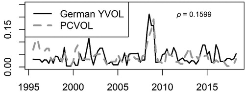
External volatility is captured as using a global measure, as well as a EU-based ‘regional’ measure. These are calculated as the four-quarter MADs for log changes in the IMF's primary commodity-price index and in German output, respectively. It is expected that increases in either might lead to increased domestic macroeconomic volatility, but specific countries and variables might be more susceptible to shocks than are others. German shocks might also be addressed through German-led policies, affecting some CEE countries more than others. These disparities, in fact, are a key focus of this study, as the effects of each (global risk, regional risk, and the transmission channel itself) are examined.

This is done by entering each country's volatility measure into a four-variable VAR (which also includes an intercept and dummies for the calculated structural breaks). VAR techniques are a common method of decomposing different types of shocks. Choi and Jung (2008), for example, use the structural VAR approach of Blanchard and Quah (1989) to assess the relative impact of domestic shocks to U.S. output volatility. Pattanachaka and Lee (2010) use a ‘counterfactual’ VAR method to uncover the sources of output volatility in six emerging markets, and find that the propagation mechanism plays more of a role than do the shocks themselves.

The VAR model estimated here includes the first difference of economic openness and the other variables in levels based on the results of the Phillips and Perron (1988) stationarity test (not reported here). The Cholesky decomposition (using a lower triangular matrix) is used in this standard, orthogonalized VAR, with the variables ordered from most exogenous to least exogenous as in Equation (1). While a VAR(1) is depicted below, each lag length is chosen by minimizing the Schwarz Criterion with a maximum of four lags.(1) $\left[\begin{array}{c}PCVO{L}_t\\ DEYVOL\\ d{\left(OPEN\right)}_t\\ MACROVO{L}_t\end{array}\right]=\left[\begin{array}{ccc}{\alpha }_{01}& \cdots & {\alpha }_{41}\\ ⋮& \ddots & ⋮\\ {\alpha }_{04}& \cdots & {\alpha }_{44}\end{array}\right]\left[\begin{array}{c}Constant\\ Breaks\\ PCVO{L}_{t-1}\\ DEYVO{L}_{t-1}\\ d{\left(OPEN\right)}_{t-1}\\ MACROVO{L}_{t-1}\end{array}\right]+\left[\begin{array}{c}{\epsilon }_{1t}\\ {\epsilon }_{2t}\\ {\epsilon }_{3t}\\ {\epsilon }_{4t}\end{array}\right]$(1) PCVOL and DEYVOL are the volatilities of commodity prices and German output, respectively, and d(OPEN) is the first difference of the trade openness measure. MACROVOL represents volatility in output, consumption, or investment, depending on the equation. Impulse-Response Functions are then generated for a one-standard-deviation shock to each variable. Forecast Error Variance Decompositions are calculated as well, to determine the relative impact of each type of exposure. The results are explained below.

4. Results

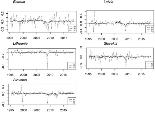
Figure 2 presents the growth rates of all three real expenditure series, for all five countries, from 1995 to 2018. As would be expected based on previous empirical evidence, investment is the most variable. There is a clear drop in all three series in 2008, corresponding to the global financial crisis. One would, therefore, expect that all volatility series would ‘spike’ around the time of the crisis and that, overall, investment volatility would be greater than that of output or consumption.

Figure 2. Log Changes, Real Expenditure Series, 1995–2018. Solid grey line = Real output; solid black line = real consumption; dotted line = real investment.

4.1. Volatility series

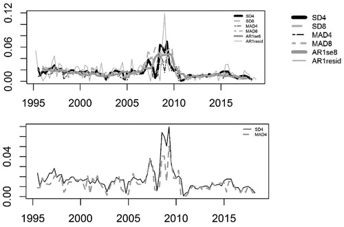
As a test case, the six alternative measures of macroeconomic volatility are compared for Latvian output. All six alternatives are plotted in the left panel of Figure 3. Each reaches its highest value in mid-2008, and all series move together. The measures calculated via an AR(1) estimation vary widely in terms of their extreme values during the crisis: the rolling standard deviations produce the smallest ‘peaks,’ while the absolute values of the residuals have the largest.

Figure 3. Alternative Volatility Measures, Latvian Output, 1995–2018. Solid line = SD4; dashed line = MAD4.

Spearman correlations among the measures are presented in Table 1. Measures with the same window length (such as SD4 and MAD4) are closely connected with one another, as are those that use the same (standard-deviation or MAD) formula. The absolute values of the AR(1) errors, which are calculated using the only method that does not apply rolling estimation methods, are least correlated with the others. In the interest of preserving as long of a time series as possible, measures that use four-quarter windows are preferred here to those that use eight-quarter windows.

Table 1. Correlations Among Alternative Volatility Measures, Latvian Output.

	SD4	SD8	MAD4	MAD8	AR1se8	AR1resid
SD4	1	0.696	0.820	0.614	0.737	0.522
SD8		1	0.558	0.867	0.974	0.424
MAD4			1	0.595	0.556	0.283
MAD8				1	0.794	0.370
AR1se8					1	0.457
AR1resid						1

The two most commonly used measures, the MAD and the MSD, are examined in more detail in the right panel of Figure 3 as well. Of the two rival methods, the former is shown to be less sensitive to shocks; it ‘peaks’ less during the 2008 financial crisis. Because it is less likely to allow a one-time shock to persist for multiple periods, MAD4 is used to measure macroeconomic volatility for all countries and variables in this study.

4.2. Structural breaks and changes across subperiods

These volatility measures, as well as structural breaks in each series and Eurozone accession and ERM membership, are plotted in Figure 4. Table 2 provides the specific break dates. As might be expected based on earlier studies which also found limited effects, structural breaks tend not to correspond to changes in the currency regime. These findings support the earlier work of Enders et al. (2013), who found little change in the volatility of the macroeconomic aggregates studied here following the introduction of the euro.

Figure 4. Volatility Measures and Structural Breaks. Dark dashed lines: Euro accession date (and ERM initiation for Slovakia and Slovenia). Other dashed lines = structural breaks (vertical) and subperiod means (vertical).

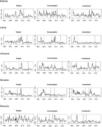
Table 2. Breakdates for Each Volatility Series.

	Volatility	Breakdates
EE	Y	2007Q2, 2010Q3
(2011)	C	2010Q1
	I	NA
LV	Y	2006Q4, 2010Q2
(2014)	C	2000Q1, 2006Q2, 2009Q4
	I	1999Q3
LT	Y	1999Q2, 2007Q1, 2010Q2
(2015)	C	2009Q3
	I	1999Q2, 2008Q3
SK	Y	2009Q1
(2009)	C	1998Q3, 2001Q4
	I	2011Q2
SL	Y	NA
(2007)	C	2008Q2, 2012Q3
	I	1999Q4

Notes: Euro accession date (January 1) in parentheses. ERM-II initiation dates = November 2005 for Slovakia and June 2004 for Slovenia.

Instead, structural breaks appear to be more closely tied to the global financial crisis and to other factors. This is particularly true in the Baltics, where structural breaks ‘bookend’ the crisis period (2006-2007 and mid-2010) for all three countries’ output volatilities, as well as for Latvian consumption volatility. These reflect the pre-crisis ‘boom’ – where EU membership helped attract capital flows, but domestic currencies’ pegs to the euro restricted adjustment and allowed for high levels of inflation – as well as the downturn that followed. While they do not have a corresponding pre-crisis structural break, Estonian and Lithuanian consumption volatility also have post-crisis breaks around 2010.

The other countries do not register similar patterns, however; Slovenian output volatility has no structural break, and breaks in Slovakia's consumption volatility all occur before 2002. While Slovakia and Slovenia joined the ERM-II and pegged their exchange rates prior to joining the Eurozone, there are no structural breaks that correspond to this change. In addition, investment behaves differently from the other two volatilities. Estonia has no breaks, while Latvia, Lithuania, and Slovenia have them in 1999, and there are post-crisis breaks only for Lithuania and Slovakia.

The means of each series during these subperiods, as well as before and after Eurozone accession, are presented in Table 3. These average values are all lower after joining the common currency. In addition, mean volatility is generally lowest in the latest subperiod, following each series’ final structural break. Only Lithuanian investment volatility rose following its 2008 break. The Kruskall-Wallis test shows that these differences in group means are indeed significant for all series across the defined structural breaks.

Table 3. Means by Subperiod and Tests for Group Differences.

			Eurozone entry			Break-defined subperiods
	Volatility	All	Pre	Post	KW (p-val.)	1	2	3	4	KW (p-val.)
EE	Y	0.010	0.012	0.006	9.345 ( 0.002)	0.010	0.022	0.006		23.023 ( 0.000)
	C	0.008	0.010	0.006	15.066 ( 0.000)	0.010	0.006			17.750 ( 0.000)
	I	0.064	0.060	0.072	3.016 (0.082)
LV	Y	0.013	0.014	0.009	5.125 ( 0.024)	0.013	0.026	0.008		26.634 ( 0.000)
	C	0.013	0.014	0.007	7.221 ( 0.007)	0.019	0.008	0.026	0.008	22.518 ( 0.000)
	I	0.080	0.084	0.065	0.372 (0.542)	0.152	0.064			17.812 ( 0.000)
LT	Y	0.010	0.010	0.008	0.208 (0.648)	0.015	0.008	0.016	0.006	31.901 ( 0.000)
	C	0.013	0.015	0.005	14.066 ( 0.000)	0.017	0.007			25.148 ( 0.000)
	I	0.069	0.067	0.080	3.025 (0.082)	0.105	0.046	0.077		29.027 ( 0.000)
SK	Y	0.009	0.013	0.004	52.659 ( 0.000)	0.013	0.003			58.389 ( 0.000)
	C	0.009	0.010	0.006	10.495 ( 0.001)	0.008	0.018	0.007		15.097 ( 0.001)
	I	0.069	0.080	0.053	11.200 ( 0.001)	0.085	0.032			33.791 ( 0.000)
SL	Y	0.009	0.009	0.010	0.129 (0.719)
	C	0.008	0.008	0.009	2.538 (0.111)	0.007	0.013	0.008		16.965 ( 0.000)
	I	0.039	0.043	0.035	0.159 (0.690)	0.068	0.032			6.549 ( 0.010)

Notes: KW: Kruskal-Wallis test for differences in group means. P-values in parentheses. Bold = significant at 5 percent.

Not all means are significantly different pre- and post-euro, however. Only Slovakia has significant differences for all three types of volatility, but this is likely due to the fact that its Eurozone accession took place during the height of the crisis. In the Baltics, the differences among means are significant for Estonian and Latvian output and consumption, as well as Lithuanian consumption. For Slovenia, on the other hand, the differences in means for consumption and investment are not significant. These results show, therefore, that while macroeconomic volatility has indeed become lower following Eurozone accession in some cases, it not necessarily because of Eurozone accession. Such causation would need to be formally tested, however.

4.3. VAR analysis and decomposition

Finally, the relative impacts of openness and external risk are examined. This will highlight the possibility that shocks have asymmetric affects across these countries. Trade openness is plotted in Figure 5. Here, the Baltics seem to behave differently from their neighbours; while all have seen openness increase over the study period, these three countries’ measures have generally decreased since 2011. This might be due to particularly rapid growth following the steep output declines immediately following the global financial crisis, which would affect the measure's denominator. The two external volatility measures, in German output and world commodity prices, are depicted in Figure 6. While they peak together during the 2008 crisis, there is little correlation between the two measures. Considering these types of risk separately, it is possible to uncover their individual effects by entering these variables into the model separately.

Figure 5. Trade Openness Measures (Exports plus Imports as Share of GDP). Dark dashed line: Euro accession date. Other dashed lines = structural breaks (vertical) and subperiod means (vertical). ERM membership shown for Slovakia (November 2005) and Slovenia (June 2004).

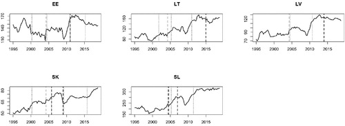
Figure 6. External Volatility Measures.

The Impulse Response Functions (IRFs) for each country's VAR are presented in Figure 7. In general, external shocks have a significant impact on all types of macroeconomic variability, more so than do changes in economic openness. This finding is largely consistent with the results of Kim (2007), which are mentioned above.

Figure 7. Impulse Response Functions to a 1-SD Shock (With ±2 S.E. Bands).

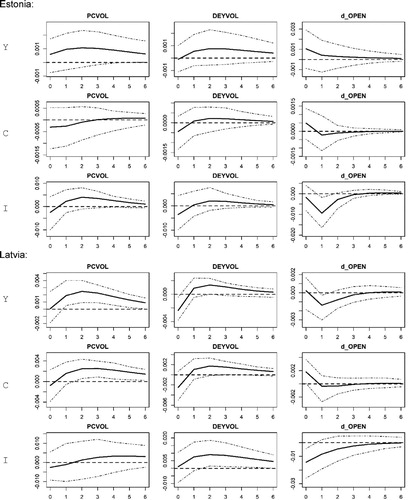
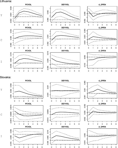
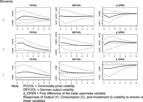
One key finding from the IRFs is that Latvia and Lithuania are particularly affected by all explanatory variables. Increases in commodity-price volatility lead to increases in both Baltic countries’ output volatilities, as well as in consumption volatility in Latvia and investment volatility in Lithuania. Regional shocks are also influential in these two economies. A positive shock to German output volatility increases all three types of macroeconomic volatility in Latvia, as well as output (and, to a limited extent, consumption) variability in Lithuania. Estonia is less affected, with only commodity-price volatility having a weak and somewhat delayed effect on output volatility. Increased openness, however, results in reduced investment variability in Estonia.

Elsewhere, only Slovakia registers a significant effect – increases in output volatility – following a positive shock to economic openness, suggesting that this channel has a limited direct influence on this set of countries. In general, the two non-Baltic countries show relatively few significant responses. Commodity-price volatility shocks spread to output and consumption volatility in Slovakia and Slovenia, respectively; German output shocks affect investment variability in Slovakia as well. But the total number of significant responses is low.

These results also show that global volatility has more influence on output volatility than does regional volatility, in all countries except Slovenia. The effects of commodity-price volatility on the other volatilities are no larger than those of German output volatility (two countries’ consumption volatilities, and one country's investment volatility, are increased following a shock). As noted elsewhere, common exposure to external shocks will allow for a more effective EU-level response.

The IRF findings are supported by the FEVDs in Table 4, with external volatility contributing a large amount to the forecast error in Latvian output and consumption volatility, for example. ‘Large’ values, defined here using a threshold of ten percent, match significant IRFs in all but a few cases (Latvian investment, Lithuanian consumption, and openness in both cases outlined above). These results confirm that Latvia and Lithuania are most susceptible to output shocks that originate in Germany.

Table 4. Forecast Error Variance Decompositions.

		Estonia				Latvia
	Horizon	PCVOL	DEYVOL	D(OPEN)	VOL	PCVOL	DEYVOL	D(OPEN)	VOL
Y	1	0.85	0.02	2.67	96.46	0.010	10.99	0.10	88.90
	4	4.61	1.91	1.91	91.00	18.49	11.68	3.25	66.51
	8	6.69	2.88	1.84	87.84	23.78	11.74	3.01	61.32
	12	7.03	3.00	1.83	87.36	24.06	11.72	3.00	61.06
C	1	0.47	0.96	1.18	97.39	0.620	6.60	3.49	89.29
	4	0.67	1.11	1.15	96.12	10.67	8.67	2.41	77.33
	8	0.73	1.26	1.14	95.88	16.58	9.49	2.17	70.82
	12	0.74	1.27	1.14	95.86	17.31	9.53	2.14	70.07
I	1	0.65	1.34	0.34	97.67	0.28	0.05	8.54	91.12
	4	3.15	1.62	7.83	87.33	0.36	4.63	6.54	86.99
	8	3.98	1.81	7.77	86.36	1.10	6.65	6.06	84.53
	12	3.99	1.81	7.77	86.34	1.30	6.86	6.02	84.15
		Lithuania				Slovakia
	Horizon	PCVOL	DEYVOL	D(OPEN)	VOL	PCVOL	DEYVOL	D(OPEN)	VOL
Y	1	2.91	1.57	1.74	93.77	9.64	0.00	0.25	90.1
	4	29.48	20.01	2.08	48.18	13.62	0.03	3.61	61.19
	8	32.88	20.28	2.01	44.51	13.87	0.05	3.94	60.41
	12	32.88	20.29	2.01	44.50	13.87	0.05	3.94	60.4
C	1	0.07	0.51	0.06	99.36	2.02	0.00	3.13	94.84
	4	2.17	4.97	1.91	90.80	1.93	1.40	2.30	89.14
	8	4.16	6.48	2.06	87.13	2.38	2.08	2.09	87.87
	12	4.45	6.57	2.06	86.74	2.42	2.19	2.06	87.72
I	1	0.00	6.23	1.24	92.53	0.43	1.21	0.23	98.13
	4	8.64	5.56	1.42	82.73	2.90	9.11	0.48	86.54
	8	11.63	5.43	1.36	79.95	2.91	10.20	0.49	85.38
	12	11.74	5.42	1.36	79.86	2.94	10.23	0.49	85.32
		Slovenia
	Horizon	PCVOL	DEYVOL	D(OPEN)	VOL
Y	1	0.13	0.01	0.16	99.70
	4	3.00	0.04	1.61	95.20
	8	3.42	0.04	1.61	94.77
	12	3.42	0.04	1.61	94.77
C	1	10.46	1.04	0.61	87.89
	4	16.58	1.09	0.76	74.84
	8	16.85	1.08	0.80	74.35
	12	16.85	1.08	0.80	74.35
I	1	2.22	0.75	2.05	94.97
	4	6.68	0.50	3.42	88.91
	8	7.92	0.48	3.45	87.66
	12	7.96	0.48	3.44	87.62

Note: PCVOL: Commodity-price volatility; DEYVOL: German output volatility; D(OPEN):  First difference of the trade openness variable.

Forecast errors of Output (Y), Consumption (C), and Investment (I) volatility.

The IRFs and FEVDs also show that external volatility spills over most to two of the three Baltic countries and that increased trade openness reduces output volatility only in a few cases. These results generally corroborate earlier findings that the trade channel does not transmit shocks, such as those of Razin and Rose (1994) and Karras (2006). There is little support for the positive relationship shown by di Giovanni and Levchenko (2009) or the effects on consumption highlighted by Buch and Yener (2010). These findings are worthy of further investigation, particularly in a model that includes financial linkages.

Differences among countries and among types of external exposure are interesting – and novel – findings of this study. In particular, Estonia's status as a technological ‘star,’ with a level of post-transition development that allowed it to be the first euro adopter in the Baltic region, sets it apart from its two Baltic neighbours. Perhaps, for this reason, it is relatively less susceptible to external shocks. Latvia's and Lithuania's connections to German shocks indicate that they might benefit more from a common policy response to a EU-wide regional shock than might the others. Divergence among these countries – as well as the rest of the region, might therefore increase.

There is some evidence of regional cohesion, however. All three Baltic countries experienced a significant reduction in consumption volatility after they joined the Eurozone (and two also saw output volatility decrease as well), so perhaps in this regard the entire sub-region benefits from Eurozone membership. While Slovakia's Eurozone membership is difficult to separate from the effects of the financial crisis, limited effects for this country suggest that there are sizable differences between, as well as within, subregions.

5. Conclusion

Membership in a common currency can be particularly attractive for small open economies because of the potential for increased stability. The loss of an independent money supply and interest rate, however, might make the country less effective in dealing with macroeconomic instability. External shocks might, therefore, have an unexpectedly large impact on these economies. Because these two effects work in opposite directions, it is necessary to investigate volatility processes empirically. Countries and sub-regions face different degrees of susceptibility to global and regional shocks, which might foment divergence within the currency area under a common monetary policy.

This study examines the volatilities of real GDP, consumption, and investment in five CEE Eurozone members, using quarterly data from 1995 to 2018. Tests for structural breaks in these time-varying volatility measures show that, in most cases, formal breaks do not specifically correspond to Eurozone accession. This is perhaps unsurprising, given the findings of previous studies. Instead, breaks capture other interesting events during this period, including the events leading up to, and following the 2008 financial crisis. Overall, 13 of the 15 volatility series – including all five consumption series – exhibit at least one structural break. Clearly the underlying volatility processes have changed over the last decades of economic transition.

Volatility means tend to be lower after joining the Eurozone, as well as following each series’ final structural break. A nonparametric test for differences in means show that all series’ averages are significantly different across structural-break regimes, but not always pre- and post-Eurozone accession. Average volatility is significantly different before and after joining the Eurozone for Slovakia, but this coincides with the Global Financial Crisis. Slovenia is not affected, and there are significant differences for Baltic consumption and output. While it is difficult to make conclusions from such a small sample, it is possible that certain benefits of Eurozone accession outweigh the costs in the Baltic region, but not elsewhere. Perhaps exchange-rate regimes play a role: Because there was no shock associated with newly implementing a fixed exchange rate, the Baltics were able to gain access to financial markets and consumption-smoothing opportunities. Additionally, as late euro adopters, they joined the group as the post-crisis recovery was in full swing. Volatility may have declined, independent of currency policy. Separating these effects must be left for future research.

Testing for spillovers from global and regional volatility to these series, this study finds that Latvia and Lithuania are most affected, and Estonia is among those that are least affected. This suggests that country differences – including growth and technical progress during the transition process, as well as the timing of Eurozone accession, might lead to different results, even for members of a defined geographic sub-region. The underlying factors behind Estonia's apparent resilience, however, must also be addressed in a future study. At the same time, external volatility appears to have more effects on output than does regional volatility, while openness itself has only a limited impact overall. Latvia and Lithuania, however, do see spillovers from regional to domestic volatility. This finding – that the Baltics are more susceptible to external shocks than elsewhere in the bloc, but at the same time might benefit most from a common policy response – might have implications on the EU's status as a unified, synchronized economic region.

Besides providing a detailed analysis of this important part of the world, this study also provides a framework for studying other regions for which common currencies or monetary policy have been implemented or are being considered. First, out of a set of feasible alternatives, a quarterly measure of macroeconomic volatility is chosen and calculated. This adds to the literature on the modelling of volatility using low-frequency data. Second, structural breaks in these series are identified using empirical methods, and these breaks can be connected to changes in policy or to other events anywhere in the world. Finally, a method of separating internal and external sources of volatility spillovers is developed.

These methods can not only be extended to future Eurozone members, they can also help inform the debate regarding currency union in Africa, Latin America, or elsewhere in the world. Those countries that are more exposed to global shocks might find themselves susceptible to ‘asymmetric’ volatility to which their currency partners are more insulated. Strong regional shocks might be successfully mitigated through a common set of policies. Such varying effects might compromise the currency union's ability to implement a unified monetary policy response.

Disclosure statement

No potential conflict of interest was reported by the author(s).

Notes on contributor

Scott Hegerty is an Associate Professor in the Department of Economics at Northeastern Illinois University in Chicago. His research interests include international macroeconomics, particularly in the Baltic region and elsewhere in Northern and Central Europe, as well as urban economic geography. He received his Ph.D. in Economics from the University of Wisconsin-Milwaukee

Notes

1 For this reason, only these two countries’ ERM start dates are noted in this study.

2 GARCH models are commonly used for volatility modeling, but require higher-frequency data and more observations than are available here. For a treatment of measurements of macroeconomic volatility in fairly low-frequency time-series data, see Bahmani-Oskooee and Hegerty (2012).

References

- Ahmed, A. D., & Suardi, S. (2009). Macroeconomic volatility, trade and financial liberalization in Africa. World Development, 37(10), 1623–1636. https://doi.org/10.1016/j.worlddev.2009.03.009
- Ang, J. B. (2011). Finance and consumption volatility: Evidence from India. Journal of International Money and Finance, 30(6), 947–964. https://doi.org/10.1016/j.jimonfin.2011.05.010
- Avouyi-Dovi, S., & Sahuc, J.-G. (2016). On the sources of macroeconomic stability in the euro area. European Economic Review, 83, 40–63. https://doi.org/10.1016/j.euroecorev.2015.11.012
- Bahmani-Oskooee, M., & Hegerty, S. W. (2012). Measures of uncertainty in economics. In P. E. Simmons & S. T. Jordan (Eds.), Economics of Innovation, Incentives and uncertainty, Nova Science Publishers (pp. 141–153). Ch.7
- Bai, J., & Perron, P. (1998). Estimating and testing linear models with multiple structural changes. Econometrica, 66(1), 47–78. https://doi.org/10.2307/2998540
- Bailey, M. J., Tavlas, G. S., & Ulan, M. (1987). The impact of exchange-rate volatility on export growth: Some Theoretical Considerations and empirical results. Journal of Policy Modeling, 9(1), 225–243. https://doi.org/10.1016/0161-8938(87)90010-X
- Barro, R., & Tenreyro, S. (2007). Economic effects of currency Unions. Economic Inquiry, 45(1), 1–23. https://doi.org/10.1111/j.1465-7295.2006.00001.x
- Bauer, C., & Herz, B. (2005). How credible are the exchange rate regimes of the new EU countries? Empirical evidence from market Sentiment. Eastern European Economics, 43(3), 55–77. https://doi.org/10.1080/00128775.2005.11041105
- Beetsma, R., & Giuliodori, M. (2010). The macroeconomic costs and benefits of the EMU and other monetary unions: An overview of recent research. Journal of Economic Literature, 48(3), 603–641. https://doi.org/10.1257/jel.48.3.603
- Blanchard, O. J., & Quah, D. (1989). The dynamic effects of aggregate demand and supply disturbances. American Economic Review, 79(4), 665–673.
- Buch, C. M., & Yener, S. (2010). Consumption volatility and financial openness. Applied Economics, 42(28), 3635–3649. https://doi.org/10.1080/00036840802260916
- Campos, N. F., Fidrmuc, J., & Korhonen, I. (2019). Business cycle synchronisation and currency unions: A review of the econometric evidence using meta-analysis. International Review of Financial Analysis, 61(1), 274–283. https://doi.org/10.1016/j.irfa.2018.11.012
- Choi, K., & Jung, C. (2008). The sources of The Decline in U.S. Output volatility. Contemporary Economic Policy, 26(1), 132–144. https://doi.org/10.1111/j.1465-7287.2007.00053.x
- De Grauwe, P., & Schnabl, G. (2005). Nominal versus real convergence – EMU entry scenarios for the new member states. Kyklos, 58(4), 537–555. https://doi.org/10.1111/j.0023-5962.2005.00301.x
- Di Giovanni, J., & Levchenko, A. (2009). Trade openness and volatility. Review of Economics and Statistics, 91(3), 558–585. https://doi.org/10.1162/rest.91.3.558
- Enders, Z., Jung, P., & Müller, G. J. (2013). Has the euro changed the business cycle? European Economic Review, 59, 189–211. https://doi.org/10.1016/j.euroecorev.2012.12.003
- Fang, W.-S., & Miller, S. M. (2008). The Great Moderation and the relationship between output growth and its volatility. Southern Economic Journal, 74(3), 819–838.
- Firdmuc, J. (2003). Economic reform, democracy and growth during post-communist transition. European Journal of Political Economy, 19(3), 583–604. https://doi.org/10.1016/S0176-2680(03)00010-7
- Gradzewicza, M., & Makarskia, K. (2013). The business cycle implications of the euro Adoption in Poland. Applied Economics, 45(17), 2443–2455. https://doi.org/10.1080/00036846.2012.667550
- Hirata, H., Kim, S. H., & Kose, M. A. (2007). Sources of fluctuations: The case of MENA. Emerging Markets Finance and Trade, 43(1), 5–34. https://doi.org/10.2753/REE1540-496X430101
- Karras, G. (2006). Trade openness, economic size, and macroeconomic volatility: Theory and empirical evidence. Journal of Economic Integration, 21(2), 254–272. https://doi.org/10.11130/jei.2006.21.2.254
- Kenen, P. B., & Rodrik, D. (1986). Measuring and Analyzing the effects of Short-Term volatility in real exchange rates. The Review of Economics and Statistics, 68(2), 311–315. https://doi.org/10.2307/1925511
- Kim, S. Y. (2007). Openness, external risk, and volatility: Implications for the compensation hypothesis. International Organization, 61(1), 181–216. doi: 10.1017/S0020818307070051
- Kodama, Masahiro. (2013). External shocks and high volatility in consumption in low-income countries, The Developing Economies, Institute of Developing Economies, 51(3), 278–302, September.
- Kose, MA, Prasad, E, Rogoff, K, & Wei, S.-J. (2009). Financial Globalization: A Reappraisal. IMF Staff Papers, 56(1), 8–62. doi: 10.1057/imfsp.2008.36
- Kruskal, W. H., & Allen Wallis, W. (1952). Use of ranks in one-criterion variance analysis. Journal of the American Statistical Association, 583–621. https://doi.org/10.1080/01621459.1952.10483441
- Lehwald, S. (2013). “Has the euro changed business cycle synchronization? Evidence from the core and the Periphery”. Empirica, 40(4), 655–684. https://doi.org/10.1007/s10663-012-9205-8
- Meller, B. (2013). The two-sided effect of financial globalization on output volatility. Review of World Economics, 149(3), 477–504. https://doi.org/10.1007/s10290-013-0156-3
- Miles, W., & Vijverberg, C.-P. C. (2018). Did the euro common currency increase or decrease business cycle synchronization for its Member countries? Economica, 85(339), 558–580. https://doi.org/https://doi.org/10.1111/ecca.12201
- Mundell, r. A. (1961). A theory of optimum currency areas. American Economic Review, 51(4), 657–665.
- Pattanachaka, K., & Lee, J. M. (2010). Sources of output volatility from financial crisis in emerging markets. Applied Financial Economics, 20(3), 183–199. https://doi.org/10.1080/09603100903282705
- Phillips, P. C. B., & Perron, P. (1988). Testing for a Unit Root in time series regression. Biometrika, 75(2), 335–346. https://doi.org/10.1093/biomet/75.2.335
- Rangvid, J., Santa-Clara, P., & Schmeling, M. (2016). Capital market integration and consumption risk sharing over the long Run. Journal of International Economics, 103, 27–43. https://doi.org/10.1016/j.jinteco.2016.08.001
- Razin, A., & Rose, A. K. (1994). “Business-cycle volatility and openness: An exploratory cross-sectional analysis. In Leonardo Leiderman & Assaf Razin (Eds.), Capital mobility: The impact on consumption, investment and growth (pp. 48–75). Cambridge University Press.
- Sahoo, P. K., Rao, D. T., & Rath, B. N. (2019). Does financial integration reduce output volatility? New evidence from cross-country data. Economic Papers: A Journal of Applied Economics and Policy, 38(1), 41–55. https://doi.org/10.1111/1759-3441.12235
- Staehr, K. (2017). The choice of reforms and economic system in the Baltic states. Comparative Economic Studies, 59(4), 498–519. https://doi.org/10.1057/s41294-017-0037-1