Volatility under the spotlight: panel regression analysis of online slots player in the UK

ABSTRACT

Volatility refers to the variability of bet outcomes in gambling and has been recognized as a potentially important influence on behavior. The research literature has developed competing ideas for how different behavioral responses to volatility might influence player risk. However, few empirical studies have investigated how volatility influences player behavior in a live-play, real-money environment. This paper studies 4,281 regular online slot players from two operators in the UK – one casino-focused, one bingo-focused. Longitudinal panel regressions analyze variation in players’ daily session time, financial loss and declined deposits as they switched among slots games with different volatilities relative to their usual play. The findings indicate that the relationship between game volatility and player behavior is complex and often non-linear. For slots players in the casino-focused sample, lower levels of volatility than usual were typically associated with lower than average losses, declined deposits and session time. However, significant relationships were not detected in the bingo-focused operator sample. Collectively, these findings suggest that while volatility may be an important influence on behavior, this influence is not necessarily uniform or easily generalized from one population of players to another.

KEYWORDS:

• Online gambling
• slots
• expenditure
• player behavior
• volatility

Introduction

A public health approach to gambling-related harm encourages consideration of three interacting factors (Productivity Commission, 1999; Shaffer & Korn, 2002). These are (i) the structural characteristics of activities (e.g. the gambling product, its look and feel and mathematical reward structure); (ii) the environment or context (e.g. venues, gambling medium or culture); and (iii) the nature of the ‘host’ (i.e. the players or consumers). So far much of the focus of regulators, research and policy has been upon players, including their characteristics and behavior. Relatively less attention has been directed to the nature of the product and the complex inter-relation between player characteristics and contextual factors. As a result, organizations such as the UK regulator, the Gambling Commission (2020a) have sought to address this imbalance by challenging industry to develop stronger guidelines for responsible product and game design, following advice from the Advisory Board for Safer Gaming and its Digital Advisory Panel (Gambling Commission, 2020b). These imperatives have encouraged a greater need for evidence-based regulation, with a particular focus on insights gained from analysis of product risk, industry-data and specific research into product features that might contribute to gambling harm.

Understanding players’ behavioral responses to different product features is an important element of assessing possible levels of risk. However, in the absence of a randomized control trial, understanding the links between product features and player behaviors in realistic commercial contexts faces a key methodological challenge. How does one know if it is the features of the game that are causing the change in behavior (exposure effect) or the characteristics of the players (selection effect)? Those who gamble on certain features might be players prone to certain behaviors, rather than seeing behavioral change driven by the features themselves. In this paper, we attempt to develop a methodology for partially addressing this challenge as applied to volatility in online slots, adopting a panel regression approach that reduces the selection effect. This methodology is more robust for identifying likely causal links than cross-sectional studies but remains limited in scope, as discussed further in the Limitations section at the end of the paper.

Volatility and gambling risk

Volatility represents the variance in pay-out over time as a gambling product is played. This characteristic is important because it affects the session-level play experience and because it can indirectly affect the cost of play for many players. While the average cost of play in a typical session is driven by the return to player (RTP) ratio of each spin, the speed of play and the average stake size, players of more volatile games can see large deviations from that average RTP (Turner, 2011). Volatility also influences cost-to-play for the majority of sessions played by the majority of players, since higher volatility games pay out in larger amounts but less frequently, concentrating the winnings into a smaller proportion of sessions and players. High volatility games, therefore, tend to have longer streaks without a material win. Holding RTP constant, loss chasing can then become a more costly activity for the majority of sessions and the majority of players, even if there is no difference in the mean average cost in aggregate across all sessions and all players (Parke et al., 2016).

Theoretically, this distinction is important because it is known that player behavior on activities such as slots can be influenced by the schedule of reinforcement (Delfabbro & Winefield, 1999; Dickerson et al., 1992). Higher volatility (and less frequent larger rewards) could potentially strengthen the partial reinforcement extinction effect (PREE) (Ferster & Skinner, 1957; Horsley et al., 2012; Skinner, 1953) and make players more resistant to extinction or periods without reward (Capaldi, 1957). The prospect of larger wins may also have the effect of encouraging chasing behavior (O’Connor & Dickerson, 2003) and may be more highly reinforcing particularly for higher risk gamblers (Knutson et al., 2001; Turner et al., 2006). This body of research suggests that gamblers, if exposed to schedules with varying degrees of volatility, should typically display greater behavioral persistence (or longer sessions) when exposed to less frequent wins (or more volatile schedule exposures). Nonetheless, it is important to note that a high volatility game may still have frequent wins, but such wins will be very small in scale compared to the large wins available, an example being national lottery syndicates with a distribution of small wins and mega prizes. Such small frequent wins may still be sufficient to provide frequent positive reinforcement for some players, depending on their thresholds for feeling rewarded by a particular win.

At the same time, there is also experimental evidence to show that the effects of less frequent or more volatile rewards operates differently when introduced in the form of concurrent schedules. Animal studies show that when subjects are exposed to a choice between schedules (1 consistent pellet on arm of a T-maze vs. 2 pellets received less frequently), animals will often prefer the smaller and more consistent rewards. Such studies show how there is a trade-off between the inter-reinforcement (rf) interval (IRI) and magnitude of reinforcement, such that leaner (less frequent rf) schedules will only attract responding when there is a compensating increase in rf magnitude. These findings are seen as consistent with Tolman’s Expectancy Value Theory (Mazur, 2016) or Incentive Theory (see Killeen, 1985).

Studies into choices between concurrent schedules involving human gambling behavior appear to yield similar results (Dixon et al., 2006; James et al., 2016) with people tending to prefer slot games with more predictable and consistent rewards. Another study conducted using confirmed pathological gamblers and non-problem gamblers found that lower reward frequency on an experimental 3-second spin-speed device reduced the time spent gambling (Linnet et al., 2010), suggesting that more volatile games might be lower risk. In a similar vein, Leino et al. (2015) found that the number of bets placed was positively associated with hit frequency and negatively associated with the size of wins, such that ‘fewer but larger payouts’ would, in general, relate to fewer bets being placed. Findings based on concurrent schedules are, however, challenged by other literature that provides evidence that big wins such as jackpots can be enticing to players, as seen in the economic modeling arguments explained by Haruvy et al. (2001) or the marginally adverse contribution of hidden jackpots to risky playing behavior identified by Donaldson et al. (2016). From this perspective, higher volatility games might be a driver of engagement and player risk, since high volatility games will typically have some big wins available. Indeed, Turner (2008) argues that increased volatility can increase losses, depending on the type of game chosen and the player’s betting strategy, potentially contributing to problematic gambling. In support of this view, Holtgrave’s (2009) analysis of adult survey data in Canada by noting that problem gambling was particularly pronounced for moderately volatile games, such as slots, although it is unclear whether it might be some other features of slots driving this correlation.

In studying volatility, it should be acknowledged that the relationship between volatility and player behavior may not be consistent and may also vary depending upon the player’s experience and approach to gambling. Moderately high game volatility has been identified as theoretically important in influencing problematic play, particularly its role in facilitating loss-chasing behavior, providing bigger, more influential wins and providing a high level of suspense and excitement (Parke & Parke, 2017). Parke et al. (2016) tentatively proposed that moderate volatility may be most related to persistent gambling, because in effect it means there is high unpredictability regarding the delivery of reinforcement, while at the same time, the chances of winning a significant sum are not grossly unrealistic. Meanwhile, a game with too high volatility may be off-putting, particularly for less experienced players or those with lower tolerance for accrued losses.

The present study

In this study, we examine the behavior of a large sample of online slot gamblers from two different operators in the UK to compare the behavior of regular players playing games with varying degrees of volatility. In order to guide this study, three hypotheses were examined: namely, that: (i) expenditure increases when players move to more volatile games; (ii) more volatile game choices are more appealing to more intensive players, in terms of having higher session time and higher spend levels; and (iii) high levels of volatility may induce more players to overspend, resulting in greater likelihood of deposits being declined by their finance provider. These hypotheses were tested by developing an analytical framework that allowed a form of within-player analysis in which the behavior of individual players is compared against their individual average across exposures to different levels of volatility.

Methodology

Data sources

Data were derived from two UK online gambling operators. The first dataset was from a casino and slots-focused operator (1/12/2017 to 10/7/2019), whereas the second dataset was from a bingo-focused operator that also provides online slots (6/9/18 to 31/12/2019). No ethical approval was required for this research because the analyses involved secondary data analysis of deidentified gambling data where there was no reasonable capacity to contact individuals to obtain consent. A waiver of consent was justified given the low risk and the fact that the results were designed to serve the public interest (contributing to an understanding of gambling-related behavior and possible harm). All datasets used were historical in nature with no contact between the authors and the dataset players prior to, during, or after the research.

To be included in the sample, all slot players had to meet a certain minimum level of engagement; namely, an expenditure of least £50 on slots on at least 7 different days spanning at least 15 calendar days over the 120 day period. A total of 10,630 players in Dataset 1 and 51,115 in Dataset 2 met these criteria. Players also had to have gambled on games for which product volatility data were available for at least 75% of their total cash wagers over the 120 day period. When this criterion was applied, a final sample of 2,622 players remained in Dataset 1 and 1,659 players in Dataset 2. The dataset is a panel, with a time axis made up of individual days gambled by a player and an entity axis made up of individual players.

Analytical strategy

A fixed effects panel regression was used to enable within sample comparisons of individual players exposed to games with varying volatility (i.e. data were nested within individuals, having rejected a random effects variant of the specification via a Hausman test). Elsewhere in gambling research, Kainulainen (2020) applied a related regression technique (‘survival regression’) to a panel dataset in order to assess the length of time it took gamblers to return to gambling following a losing day, being an attractive approach that controls for player level idiosyncrasies.

The fixed effects regression makes it possible to examine whether various behavioral parameters changed if players shifted their slots wagering toward a different mix of slot games (their ‘game mix’) with a higher or lower volatility. A range of dependent variables are used to capture daily player behavior based on the calendar day in which the relevant session begins (to account for evening sessions which span into the following morning). The three player behavior outcome variables were (i) Total slots session time per day (measured in hours); (ii) Total slots financial loss per day (measured in pounds); and (iii) Whether the player had a declined deposit on that calendar day (0/1).

The principal independent measure was a measure of volatility based on the standard deviation of the RTP resulting from a single bet, as simulated across a very large number of bets (typically a billion), represented on a scale of 1 to 8. Since volatility is, by this mathematical definition, lower across bundles of bets rather than single bets (Turner & Shi, 2015), the measure is calculated using spins at max lines, where players are able to vary the number of lines being bet on simultaneously (effectively representing a bundle of identical bets in the vast majority of games). A very small number of Playtech slots (<1% of those with data) have dynamic volatility, in the sense that it can vary depending on set-up or player choices. Play on these games is excluded from the analysis, as with play on games for which volatility feature data are not available. Volatility was included both as a linear and a squared term allowing a non-linear association with the dependent variables, given the argument from the literature that ‘moderate’ volatility might have greater risk for some players than ‘high’ volatility.

In order to compare game feature data (which exists at the game level) such as volatility to a player’s overall behavior on that day, it was necessary to convert multiple sessions of play across multiple games on the same day into a single metric. To do this, we use a stake-weighted feature average (SWFA) which creates a single value for each day for each player, based on averaging the volatility value of all the games they played that day, weighted by the amount staked on each game. In constructing the SWFA, we weight the cash stake spent on each game to adjust for the recency with which a game was launched to account partially for promotions and marketing spend around launch, since some games may attract more spend around launch in a way that is largely unconnected to whether the game features inspire particular play behaviors. To do this, games are grouped into several periods of time since launch (0–3 days, 4–7 days, 8–14 days, 15–28 days, 29–56 days, 57–120 days and 121+ days) and specified as dummy variables in an OLS regression run across all game sessions to identify the average coefficients that relate game recency to log cash bet. The cash stake on each game session for a particular player is then deflated by dividing it by exponentiated value of the relevant coefficient for the period of time corresponding to the days since that particular game was launched.¹ Results were robust to whether the weighting was done by different combinations of cash and bonus spend, so the simplest method (cash spend) was applied. Note all further references to volatility in this paper refer to volatility as adjusted by this method.

Finally, we include various calendar time controls – dummy terms to capture the day of the week, the week of the year and whether the day is a common pay day (last Friday and last working day of the month). While these calendar controls are typically not statistically significant across the whole dataset, they allow for the possibility that some weeks of the year (e.g. Christmas, major sporting events) and some days of the week (e.g. Friday nights, Sundays, payday) might drive player behaviors and outcomes in a way that is independent of the features of the games they play. Robust clustered standard errors are applied to all reported regression models, following a 0.001 p-value on a modified Wald test for groupwise heteroskedasticity identified in the sample-based specification testing.

The resulting model is a standard time-demeaned fixed effects panel regression, as described in Equation (1)(1) $\left(y_{it}-{\bar{y}}_i\right)=\beta \left(x_{it}-{\bar{x}}_i\right)+\left(u_{it}-{\bar{u}}_i\right)$(1) and estimated via ordinary least squares, implemented in Stata/IC 15.1:

(1) $\left(y_{it}-{\bar{y}}_i\right)=\beta \left(x_{it}-{\bar{x}}_i\right)+\left(u_{it}-{\bar{u}}_i\right)$(1)

where ${\mathrm{y}}_{\mathrm{i}\mathrm{t}}$ is the dependent variable for player i at time t, ${\mathbf{x}}_{\mathrm{i}\mathrm{t}}$ is the vector of independent variables for player i at time t, $\beta$ is the vector of coefficients of the independent variables, and ${\mathrm{u}}_{\mathrm{i}\mathrm{t}}$ is the model error term. ${\overline{\mathrm{v}\mathrm{a}\mathrm{r}}}_{\mathrm{i}}$ represents the average value of the specified variable for player i across all time periods t that player i played. Only days on which a player played are included in the dataset (unbalanced panel regression). The time-demeaning approach serves to remove idiosyncratic, player-level fixed effects from the dataset. Three models are estimated on each dataset, where y is respectively session time per day, financial loss per day or whether a declined deposit took place that day. The vector of 61 independent variables remains constant across models and captures: SWFA volatility, SWFA volatility squared, whether or not the day was a common pay day, six dummy variables reflecting the day of the week the gambling took place, and 51 dummy variables reflecting the week of the year, as well as a constant term.

Results

Descriptive statistics

The mean across players of the individual player average daily volatility (i.e. the grand mean in the panel data) was 3.3 for Dataset 1 and 2.9 for Dataset 2 (see Table 1). A t-test for independent samples indicated that players in Dataset 1 played more volatile slots on average than players in Dataset 2 (p < .001; see Table 1 for details).

Table 1. Descriptive results for two operator data-sets

	Operator/Data-set 1 (casino-focused brand)	Operator 2/Data-set 2 (bingo-focused brand)	p-level^a
Number of qualifying players for analysis (n)	2,622	1,659	n.a.
Player level average; median [standard deviation*]
Volatility (scale 1–8; where 8 is high volatility)	3.3; 3.1 [0.9]	2.9; 3.0 [0.7]	< .001
Session time (hours per day)	0.9; 0.5 [1.1]	0.2; 0.0 [0.9]	< .001
Total loss (GBP per day)	£50; £15 [£368]	£6; £1 [£42]	< .001
Probability of a declined deposit per day	12%; 0% [19%]	4%; 0% [9%]	< .001

* Note this is the standard deviation across player-level averages, not the average of player-level standard deviations, which is 0.6 for Operator 1 and 0.4 for Operator 2.

^aresults based on t-test for independent samples (equal variances not assumed).

A total of 95% of game play in Dataset 1 and 96% in Dataset 2 involved an average daily volatility exposure of between 2 and 5 on the 1–8 scale. In addition, most players’ daily experience of volatility deviates little from their average, suggesting players tend to stick to games with a similar volatility. For instance, the average range between a player’s maximum volatility and their minimum was 1.8 on Dataset 1 (interquartile range from minimum to maximum daily experience across players of 1.0 to 3.0) and 1.3 on Dataset 2 (interquartile range of 0.6 to 2.0). Similarly, the player-level volatility exposure average standard deviation was 0.6 on Dataset 1 and 0.4 on Dataset 2. Put another way, 51% of players in Dataset 1 played a mix of games where the average volatility was within 0.5 of their personal average on 75% or more of the days they played. Framed in a different way, 79% of players were within 1.0 of their personal average by the same criterion (67% and 92% for Dataset 2).

Players on Dataset 1 were, on average, longer-playing, higher-staking, and had more declined deposits than players on Dataset 2 as based on t-test comparisons (p < .001; see Table 1 for details). In Dataset 1, the grand mean of session time was about 1 hour spent playing per day losing a total of £50, whereas it was only 10 minutes and a £6 loss for Dataset 2 players. A total of 25% of the players in Dataset 2 had at least one day with a declined deposit over the period analyzed, with a grand mean average of any one day having a declined deposit being 4%, compared with 42% and 12% in Dataset 1.

Analytical results

Table 2 describes the relationship between changes in volatility and correlated changes in behavior at the player-level. Players from the two operators responded differently to volatility. In Dataset 1, the relationships between volatility and session time, financial loss and declined deposits were statistically significant. By contrast, in Dataset 2, the relationships were non-significant with only one relationship approaching significance (p < . 10); namely, volatility and the probability of a declined deposit.

Table 2. Results of six fixed-effects models

	Operator 1/Data-set 1 (casino-focused brand)			Operator 2/Data-set 2 (bingo-focused brand)
	Session Time (hours per day)	Total Loss (GBP per day)	Probability of a declined deposit per day	Session Time (hours per day)	Total Loss (GBP per day)	Probability of a declined deposit per day
Volatility – Linear term coefficient	0.107***	43.41**	0.0370***	0.032	1.67	−0.012
Volatility – Squared term coefficient	0.014***	−4.92**	−0.005***	−0.013	−0.23	0.002*
Volatility p-value^a	0.00	0.04	0.01	0.15	0.87	0.09
Sample size: # players [# gambling days in analysis]	2,622 players [35,491 days]	2,622 players [35,491 days]	2,622 players [35,554 days]	1,659 players [32,801 days]	1,659 players [32,801 days]	1,659 players [32,801 days]
R^2	32.2%	10.8%	30.2%	16.3%	3.1%	16.8%

*** Significant at 1% level; ** Significant at 5% level; * Significant at 10% level.

^aWald test of the null hypothesis that both the linear and squared term coefficients are jointly zero.

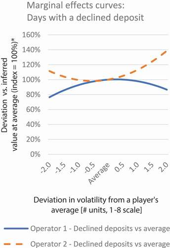
For most variables, the relationships are non-linear in that the squared term has similar levels of statistical significance to the linear term. In order to better understand the non-linear relationship, the marginal effects curves for both operators are plotted in Figures 1–3. Figure 1 plots financial loss per day; Figure 2 plots total session time per day; and Figure 3 plots the proportion of days with declined deposits. To enable comparison between the operators, the implications of increasing or decreasing volatility relative to players’ individual average exposure (x-axis) are plotted as percentage changes relative to the inferred value at that average level, which is indexed as 100% (y-axis). The x-axis range of −2 to +2 units of volatility around a player’s individual average captures over 95% of the variation experienced by players.

Figure 1. Marginal effects curves: loss per day

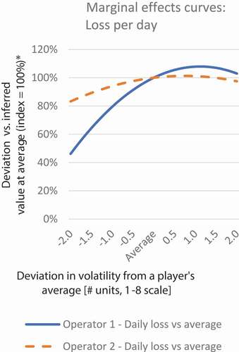
Figure 2. Marginal effects curves: session time per day

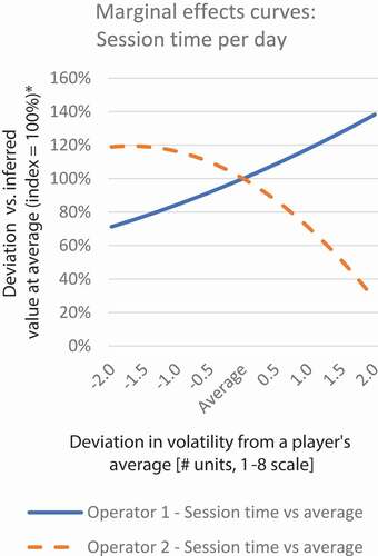
Figure 3. Marginal effects curves: days with a declined deposit

* Marginal effects curve anchor all changes relative to the inferred value at the grand mean volatility value for that operator (see Table 2 for grand mean values). Y-axis inferred values representing the 100% point are, for Operators 1 and 2, respectively, are: £77.23, £9.52 (Figure 1); 1.2 hrs, 0.2 hrs (Figure 2); and 11%, 4% (Figure 3). Please note that the dashed lines for Operator 2 all fail to be significant at the 5% level or better and the detail of the curve cannot be relied upon.

Figure 1 reveals that increasing volatility is typically associated with increased losses (only statistically significant for Operator 1), particularly by comparison between below-average and around average levels of play. For instance, Figure 1 addresses the link between volatiltiy exposure and financial losses. For Operator 1 (solid curve), a decrease of one standard deviation in volatility exposure (0.6 units) from a player’s average is associated with an average 11% reduction in loss, the equivalent of £8 per day on average.² When we examine increases in volatility exposure above a player’s average, the curve flattens, such that a one standard deviation increase above average translates into an average £5 increase in daily loss. For Operator 2 (dotted curve), one standard deviation (0.4 units) in lower volatility exposure was associated with a 1% decrease, worth an average of 17p per day, declining to a 10p increase for a one standard deviation increase in volatility above a player’s personal average volatility exposure. These marginal effects are much smaller for Operator 2 and fail to be statistically significant (p-value 0.87).

On daily session time, Figure 2, the two operators showed opposite patterns to each other. Session time increases with volatility for Operator 1 (p < .001), an average of 7 min extra per day at the player’s average exposure to volatility relative to one standard deviation below that average. For Operator 2, there is a downward trend in session time, although this was not significant (p = 0.15). The results for declined deposits (Figure 3) are the most complex of the three. For this variable, there were non-linear patterns around the average that are opposite for both operators. Increases in volatility relative to the average generally increased declined deposits (p < 0. 01) in Dataset 1, but were not significant at the 5% level for Dataset 2 (p = 0.09).

Discussion

The aim of this study was to investigate the behavioral response by online slots players as they shifted to playing lower or higher volatility games.

The research focused on three hypotheses. Hypothesis 1, that expenditure would be higher on more volatile games, was supported by the data from Operator 1, but not for Operator 2. Some indirect support was obtained for Hypothesis 2 in that more volatile game choices may be associated with higher spending and longer playing players. This is based on the observation that Operator 1 players have higher levels of spend and time spent online, and tend to play more volatile slots than Operator 2 players. Hypothesis 3 is rejected, because volatility does not appear to have a monotonic relationship with declined deposits for either Operator 1 or Operator 2. For Operator 1, both higher and lower volatility than usual were typically associated with fewer declined deposits (p-value 0.01); for Operator 2, both were associated with more declined deposits (p-value 0.09).

The findings, therefore, highlight the importance of operator characteristics and different player populations on both the nature of gambling behavior observed and the relationships between variables, as well as the meaningful non-linearity and possible non-monotonicity in some of the relationships. The notion of game interest peaking at moderate-high volatility before declining is somewhat consistent with theory put forward by Turner (2011) and Parke et al. (2016). From this perspective, if games are too volatile and initial losing streaks too long compared to what players have become used to, the game may become frustrating for the player. This declining pattern was observed weakly in both operators on financial loss, but not consistently across the other behaviors examined for each operator, pointing toward the need for a more complex, player-contingent theory of volatility that describes different relationships across time spent playing, money spent, and other risk-related behaviors.

It is also important to stress that this paper focused on short-term changes in behavior, daily variations in play given daily variations in volatility exposure, whereas some of the behavioral literature suggests that volatility is perhaps more likely to encourage riskier play in studies of gambling behavior over longer periods of time (e.g. Horsley et al., 2012). This points toward one possible explanation of the differences between the datasets. Since Operator 1 players typically play for longer periods of time each day, there may be more potential for volatility exposure to influence their behavior, hence the statistically significant relationships. However, the differences in significance may also reflect different sample sizes. Indeed, the qualitative differences between Datasets 1 and 2 may reflect qualitatively different responses to volatility in the two sets of players, casino-focused vs bingo-focused, that are not simply reflected in quantitative differences such as length of exposure to the product. Such possibilities would need to be explored in future research, using a mixed set of approaches.

Limitations and future research

It is important to acknowledge a number of issues when interpreting the findings in this paper. We have investigated the average links between volatility in online slots and player behaviors, exploiting a longitudinal panel regression technique, testing robustness to bonus spend, when games were released, calendar and pay-day patterns. This technique adjusts for player idiosyncrasies by comparing each player against their own personal average, providing a tighter grasp on causality than enabled in cross-sectional analyses. However, findings nonetheless remain associative and are only indicative of possible causal relationships, rather than formally demonstrative of them. For instance, it is possible that players possess preexisting characteristics or playing styles that influence how they behave when trying new games or games they play less frequently. One outcome might be a particular set of players with a tendency to try out games with greater variation in volatility whose behaviors then have a greater influence on the magnitude of coefficients observed in regression analysis. Panel regression requires repeat players with a reasonable number of days play data. Players who churn quickly, some of whom may be at high risk, need a different type of analysis to the one set out in this paper.

A second issue is that this study had to work with a reduced sample size due to games for which volatility feature data are not available. Third, the study was also based upon data drawn from two operators that may differ from others in the market. A fourth issue is that the study did not have the capacity to examine independent measures of harm such as might be obtained from self-report surveys of customers that could then be linked to the objective gambling data.

A number of these issues could be addressed in future studies. For example, the panel regression technique could be extended to consider lagged variables, capturing the possibility that players might seek to catch up yesterday’s losses in riskier play today or that exposure to volatility might influence gambling behaviors over a longer period of time than a day. Adjustments for bonus play, calendar features and game launch date could also be developed in a more sophisticated manner, allowing for non-linearities, contingencies and subsample variation in how such features influence cash staking. Future research could also increase the range of games included in the analysis. An increase in the universe of games for which feature data are available will mean a greater proportion of players can be analyzed with higher coverage of their staking activity, increasing the validity of findings. Alternatively, behaviors could be analyzed purely at a session level, focusing just on games with valid feature data. Independent and triangulated measures for gambling harm would allow the analysis to address harm directly. For instance, high-priority data would include players flagged by customer service staff as at risk from their gambling activity, players identified by treatment providers, and players responding to a survey identifying concerns about their gambling.

Future studies could also apply the methodologies used in this paper to a diverse set of game features and controlling for patterns between game features. Analysis of different measures of volatility, volatility relative to RTP and of game features (i.e. game events or modifiers that typically result in a higher RTP period of play) also has the potential to provide a deeper understanding of game experience. It may also be important to examine win distribution in more detail than a single volatility metric. For instance, the relative hit frequency of low, medium and large-sized wins can combine in very different ways to produce the same volatility metric, but might have important variations in the play experience and subsequent player behaviors. Finally, it will also be important to apply the technique to additional datasets, further explore group heterogeneity (such as subgroups with a high baseline level of risk or high volatility play, or possible moderating factors such as gender, age and experience with slots play), and check sensitivity to outliers to test the generalizability of the findings.

Within-player analyses can be usefully supplemented by between-player and between-product analyses. Such quantitative findings should also be blended with qualitative or more descriptive work, such as interviews with players and retrospective discussions of their play sessions, to inform resulting interpretations and recommendations. For example, visualizations of a targeted sample of higher risk players could provide more nuanced insights into the ways in which behavior changes in relation to game characteristics. Players might, for example, be asked to justify their choice of games or be asked to speak aloud their thoughts or decision-making during the course of a game during real-time play.

Competing interests

Chris Percy, Simo Dragicevic and Kiril Tsarvenkov are contracted with Playtech Plc, a B2B and B2C gambling services provider.

Paul Delfabbro and Jonathan Parke are academics and consultants active in the gambling sector, who do and seek to do paid work with a wide range of sector stakeholders, including gambling operators, regulators, harm-prevention charities and other organizations.

Acknowledgements

We would like to thank Playtech Plc and partners for making the data available for this analysis.

Data availability statement

Data are not available due to player privacy and operator commercial restrictions, as permissions only exist for analysis within Playtech Plc and the partner operators.

Disclosure statement

Chris Percy, Simo Dragicevic and Kiril Tsarvenkov are contracted with Playtech Plc, a B2B and B2C gambling services provider.

Paul Delfabbro and Jonathan Parke are academics and consultants active in the gambling sector, who do and seek to do paid work with a wide range of sector stakeholders, including gambling operators, regulators, harm-prevention charities and other organizations.

Additional information

Funding

There was no specific grant or project funding for this work. Chris Percy, Simo Dragicevic and Kiril Tsarvenkov contributed to this paper as part of their contracts with Playtech Plc, a B2B and B2C gambling services provider. Paul Delfabbro and Jonathan Parke received no funding from Playtech Plc or any other specific source for their contributions to the paper. Playtech Plc and partners made the data available for this analysis.

Notes on contributors

Chris Percy

Chris Percy is a data science contractor and independent researcher, with recent projects with the World Bank, the OECD, and the ILO. His work with Playtech and the gambling industry focuses on R&D initiatives to improve the identification and mitigation of gambling-related risk.

Kiril Tsarvenkov

Kiril Tsarvenkov is a data science professional with two masters degrees in Finance and Data Science. His work at Playtech focuses on different characteristics of game design such as volatility, max stake, autoplay and other features of interest.

Simo Dragicevic

Simo Dragicevic is founder of BetBuddy, a subsidiary of Playtech Plc, as well as Managing Director of Playtech Protect and Head of Playtech AI. He has contributed research in the areas of gambling products, safer and responsible gambling, and explainable AI. He is a PhD supervisor at City, University of London and a board member of the Responsible Gambling Council of Ontario, Canada.

Paul H Delfabbro

Paul H Delfabbro graduated from the University of Adelaide with a PhD in psychology. He has published extensively in several areas, including the psychology of gambling, child protection and child welfare and applied cognition. He has over 320 publications in these areas including over 230 national and international refereed journal articles.

Jonathan Parke

Jonathan Parke is the director of Sophro Limited, and a social psychologist interested in gambling behavior. His primary research interests include product designs, gambling motivation and principles of behavioral science, and their relationships with gambling behavior and related harms. He received his PhD in psychology from the Nottingham Trent University.

Notes

1. For instance, if on a particular day a player wagered £10 on Game A with a volatility of 4 and £30 on Game B with a volatility of 3, the player’s SWFA volatility for that day would be 3.25, weighted toward the volatility value of Game B since they wagered more of their money on that game. SWFA can also be adjusted for game recency. For instance, if Game B had been launched yesterday whereas Game A was a long-standing game, the wagering on Game B is down-weighted to reflect the fact that some play may represent promotional or curiosity play, rather than engagement with its features. The log-linear OLS model coefficient in this case is ~1.5 for Dataset 1, so the £30 wager is treated as £20 and the subsequent SWFA is 3.33.

2. The 11% applies with reference to the inferred value of loss per day at the grand mean value of volatiltiy, i.e. £77.

References

- Capaldi, E. J. (1957). The effect of different amounts of alternating partial reinforcement on resistance to extinction. American Journal of Psychology, 70(3), 451–452. https://doi.org/https://doi.org/10.2307/1419584
- Delfabbro, P. H., & Winefield, A. H. (1999). Poker machine gambling: An analysis of within session characteristics. British Journal of Psychology, 90(3), 425–439. https://doi.org/https://doi.org/10.1348/000712699161503
- Dickerson, M., Hinchy, J., Legg-England, S., Fabre, J., & Cunningham, R. (1992). On the determinants of persistent gambling behaviour: High frequency poker machine players. British Journal of Psychology, 83(2), 237–248. https://doi.org/https://doi.org/10.1111/j.2044-8295.1992.tb02438.x
- Dixon, M., MacLin, O., & Daugherty, D. (2006). An evaluation of response allocations to concurrently available slot machine simulations. Behavior Research Methods, 38(2), 232–236. https://doi.org/https://doi.org/10.3758/BF03192774
- Donaldson, P., Langham, E., Rockloff, M. J., & Browne, M. (2016). Veiled EGM jackpots: The effects of hidden and mystery jackpots on gambling intensity. Journal of Gambling Studies, 32(2), 487–498. https://doi.org/https://doi.org/10.1007/s10899-015-9566-6
- Ferster, C., & Skinner, B. F. (1957). Schedules of reinforcement. Appleton-Century Crofts.
- Haruvy, E., Erev, L., & Sonsino, D. (2001). The medium prizes paradox: Evidence from a simulated casino. The Journal of Risk and Uncertainty, 22(3), 251–261. https://doi.org/https://doi.org/10.1023/A:1011183001837
- Holtgrave, T. (2009). Gambling, gambling activities, and problem gambling. Psychology of Addictive Behaviors; Journal of the Society of Psychologist in Addictive Behaviours, 23(2), 295–302. https://doi.org/https://doi.org/10.1037/a0014181
- Horsley, R., Osborne, M., Norman, C., & Wells, J. (2012). High-frequency gamblers show increased resistance to extinction following partial reinforcement. Behavioral Brain Research, 229(2), 438–442. DOI:https://doi.org/10.1016/j.bbr.2012.01.024
- James, R. J. E., O’Malley, C., & Tunney, R. J. (2016). Why are some games more addictive than others: The effects of timing and payoff on perseverance in a slot machine game. Frontiers in Psychology, 7, Article 46. https://doi.org/https://doi.org/10.3389/fpsyg.2016.00046
- Kainulainen, T. (2020). Does losing on a previous betting day predict how long it takes to return to the next session of online horse race betting? Journal of Gambling Studies. https://doi.org/https://doi.org/10.1007/s10899-020-09974-x
- Killeen, P. R. (1985). Incentive theory. IV. Magnitude of reward. Journal of the Experimental Analysis of Behavior, 43(3), 407–417. https://doi.org/https://doi.org/10.1901/jeab.1985.43-407
- Knutson, B., Adams, C. M., Fong, G. W., & Hommer, D. (2001). Anticipation of increasing monetary reward selectivity recruits nucleus accumbens. Journal of Neuroscience, 21(16), 1–5. https://doi.org/https://doi.org/10.1523/JNEUROSCI.21-16-j0002.2001
- Leino, T., Torsheim, T., Blaszczynski, A., Griffiths, M., Mentzoni, R., Pallesen, S., & Molde, H. (2015). The relationship between structural game characteristics and gambling behavior: A population-level study. Journal of Gambling Studies, 31(4), 1297–1315. https://doi.org/https://doi.org/10.1007/s10899-014-9477-y
- Linnet, J., Thomsen, K., Møller, A., & Callesen, M. (2010). Event frequency, excitement and desire to gamble, among pathological gamblers. International Gambling Studies, 10(2), 177–188. https://doi.org/https://doi.org/10.1080/14459795.2010.502181
- Mazur, J. E. (2016). Learning and behaviour. Routledge.
- O’Connor, J., & Dickerson, M. (2003). Definition and measurement of chasing in off-course betting and gaming machine play. Journal of Gambling Studies, 19(4), 359–386. https://doi.org/https://doi.org/10.1023/A:1026375809186
- Parke, J., & Parke, A. (2017). Getting grounded in problematic play: Using digital grounded theory to understand problem gambling and harm minimisation opportunities in remote gambling. GambleAware. Retrieved June 1, 2020, from https://about.gambleaware.org/media/1610/parke-parke-2017-gtr.pdf
- Parke, J., Parke, A., & Blaszczynski, A. (2016). Key issues in product-based harm minimisation: Examining theory, evidence and policy issues relevant in Great Britain. GambleAware. Retrieved June 1, 2020, from https://about.gambleaware.org/media/1362/pbhm-final-report-december-2016.pdf
- Productivity Commission. (1999). Australia’s gambling industries.
- Shaffer, H. J., & Korn, D. A. (2002). Gambling and related mental disorders: A public health analysis. Annual Review of Public Health, 23(1), 171–212. https://doi.org/https://doi.org/10.1146/annurev.publhealth.23.100901.140532
- Skinner, B. F. (1953). Science and human behaviour. MacMillen.
- The Gambling Commission. (2020a). Gambling commission sets the industry tough challenges in race to accelerate progress to raise standards and reduce gambling harm. Retrieved June 1, 2020, from https://www.gamblingcommission.gov.uk/news-action-and-statistics/News/gambling-commission-sets-the-industry-tough-challenges-in-race-to-accelerate-progress-to-raise-standards-and-reduce-gambling-harm
- The Gambling Commission. (2020b). The gambling commission publishes independent advice from its expert advisory groups to reduce online gambling harm. Retrieved June 1, 2020, from https://www.gamblingcommission.gov.uk/news-action-and-statistics/News/the-gambling-commission-publishes-independent-advice-from-its-expert-advisory-groups-to-reduce-online-gambling-harm
- Turner, E. N. (2008). Games, gambling and gambling problems. In M. Zangeneh, A. Blaszczynski, & N. E. Turner (Eds.), The pursuit of winning: Problem gambling theory, research and treatment (pp. 33–64). Springer.
- Turner, N. E. (2011). Volatility, house edge, and prize structure of gambling games. Journal of Gambling Studies, 27(4), 607–623. https://doi.org/https://doi.org/10.1007/s10899-011-9238-0
- Turner, N. E., & Shi, J. (2015). The relationship between game volatility, house edge and prize structure of gambling games and what it tells us about gambling game design. International Journal of Computer Research, 22(2), 107–131.
- Turner, N. E., Zangeneh, M., & Littman-Sharp, N. (2006). The experience of gambling and its role in problem gambling. International Gambling Studies, 6(2), 237–266. https://doi.org/https://doi.org/10.1080/14459790600928793