Point-of-interest recommendation using extended random walk with restart on geographical-temporal hybrid tripartite graph

ABSTRACT

Previous studies neglected the impact of shared spatio-temporal interests in the Point of Interest (POI) recommendation. The proposed GHTG-ERWR method simultaneously models shared spatio-temporal preferences of users, the dynamics of users’ behavior, and the geographical effect for POI recommendation. It is composed of an Extended Random Walk with Restart (ERWR) algorithm that works on a Geographical-temporal Hybrid Tripartite Graph (GHTG). The method overcomes shortcomings of prior approaches by employing users’ joint preferences over time and space through the auxiliary information derived from location-session and session-location edges. Experimental results on Gowalla and Weeplaces datasets proved the feasibility of the approach.

KEYWORDS:

• Location-based social networks (LBSNs)
• graph-based recommendation
• spatio-temporal graph
• random walk with restart (RWR)
• common spatio-temporal preferences

1. Introduction

Location-based social networks (LBSNs), such as Gowalla, Foursquare, and Weeplaces, have revolutionized how we access and exploit spatial information in our daily lives. LBSNs have enabled users to check in and share their experience of visited venues for any point-of-interest (POI) using mobile devices. Having the check-in data, LBSNs have also been able to mine users’ previous activities, extract their preferences, and dynamically recommend new POIs to the users. Due to its significance for personalization and business/service advertisement, several researchers have recently studied and enhanced different aspects of POI recommendation systems (Li et al. 2014, Sun et al. 2015, 2019, Litou et al. 2017, Orso et al. 2017, Xia et al. 2017, Yu et al. 2017a, Valverde-Rebaza et al. 2018, Si et al. 2019).

Studying the check-in data reveals that there is a constant change in the users’ interests, behaviors, and preferences over time and space. The dynamics of users’ choices have a severe impact on the accuracy of POI recommendations (Rafailidis et al. 2017). Therefore, exploring and exploiting users’ check-in history can contribute to a more personalized POI recommendation based on the users’ current needs and desires.

Currently, two serious challenges of POI recommendation in LBSNs are related to handling the data sparsity (Niu et al. 2016, Rafailidis et al. 2017, Wang et al. 2017, Yu et al. 2017b, Kefalas et al. 2018, Luo et al. 2019, Yang et al. 2019) and capturing the users’ preferences (Ding and Li 2005, Koren 2009, Rafailidis et al. 2017, Yang et al. 2019, Lyu et al. 2019, Qi et al. 2019). The problem of sparse user-item matrix, as a result of limited number of visited POIs by each user, becomes even more serious when a user travels to a distant place, as most of the POIs visited by them are usually located in the immediate vicinity of their home (Wang et al. 2017). Another issue is the problem of capturing user’s preferences at different times and locations as the users’ behaviors are inclined to vary due to several unpredictable factors (Rafailidis et al. 2017).

Various approaches have been put forward to simultaneously address the above-mentioned challenges. Initial works focused primarily on content-based filtering (CB) (Popescul et al. 2001, Melville et al. 2002) and collaborative filtering (CF) (Popescul et al. 2001, Melville et al. 2002, Yang et al. 2014, Yu et al. 2017b, Kant and Mahara 2018), among which models like time weight CF (Ding and Li 2005), timeSVD++ (Koren 2009), TMF and BTMF (Zhang et al. 2014), TGSC-PMF (Ren et al. 2017), CTF-ARA (Si et al. 2017) can be pointed out. For example, STELLAR was proposed as a tensor-based algorithm for successive POI recommendations in LBSNs (Zhao et al. 2016). This model uses a four-tuple ranking-based pairwise tensor factorization framework to deal with the data sparsity issue. Chen et al. (Chen et al. 2016) proposed a third-rank tensor to incorporate three important factors, including successive behavior, locality behavior, and group preferences, to recommend POIs (Chen et al. 2016). A temporal-aware POI recommendation system based on a three-dimensional tensor (user, category, and time) was also presented to alleviate the data sparsity, facilitate user’s travel to a new city, and model the user’s preferences (Ying et al. 2017). The model is composed of two components: context-aware tensor decomposition for user preference modeling and weighted HITS (Hypertext Induced Topic Search) POI rating. LRT (Gao et al. 2013) is another location recommendation framework proposed to use user behavior’s temporal patterns for the POI recommendation. This framework is based on low-rank matrix factorization and has three main steps of temporal division, factorization, and aggregation. gSCorr (geo-social correlation) (Gao et al. 2012) was also presented to handle the cold start problem in location recommendation through different correlation probabilities calculated from geo-social properties.

In another direction, graph-based methods were presented as a pragmatic solution to model the interactions between users and items. These methods calculate the similarity of nodes from a more general perspective rather than using the neighborhood pairs or local calculations (Xiang et al. 2010). Graph-based recommender systems have used either pure temporal (Xiang et al. 2010, Yu et al. 2014, Nzeko’O et al. 2017, Musto et al. 2017, Guo et al. 2018, Liu et al. 2019, Zhou and Han 2019) or spatio-temporal (Yuan et al. 2014, Kefalas et al. 2018) methods. The temporal methods only rely on the time of users’ check-ins for generating the graph, while spatio-temporal methods use both the time and locations of users’ check-ins in generating the graph.

As an example of temporal approaches, STG (session-based temporal graph) was proposed by Xiang et al. (Xiang et al. 2010) and introduced the concept of session nodes. Session nodes are generated in STG to represent the users’ activity (i.e. rating, like or dislike items, or visiting locations) at a specific time slot. Using the session nodes, STG models both short-term and long-term preferences of the users via session-item and user-item edges, respectively. Despite its merits, STG fails to consider the specific characteristics of each item and therefore incurs a considerable loss of information. In response to this issue, Yu et al. (2014) introduced Topic-STG to recommend personalized tweets to users by adding topic nodes to STG (Yu et al. 2014). Using topic nodes and creating new connections such as topic-user, topic-tweet, and topic-session, they were able to consider textual information, temporal effect, and users’ behavior in the tweet recommendation process. However, Topic-STG does not consider the age of the edges in their weighting schemes. Therefore, Nzeko’O et al. (Nzeko’O et al. 2017) presented Time Weight Content-based STG to calculate the weightings of the edges based on their ages. Finally, Najafabadi et al. (2019) proposed an algorithm that incorporates the visiting time into the graph structure and uses a hybrid CF algorithm to suggest top-N items to the users.

By focusing only on time, the studies mentioned above have neglected the importance of location and spatial effects on the recommendation process. Recently, some graph-based methods have been proposed that consider both time and location in their recommendation methods. Yuan et al. (2014) proposed a technique called GTAG-BPP that uses the Breadth-First Preferences Propagation (BPP) algorithm to calculate the value of preferences for each location and recommends the top-N POIs based on Geographical-Temporal influences Aware Graph (GTAG). GTAG includes User, Location, and Session nodes and three types of edges, including POI-POI, user-session, session-user, session-location, and location-session. The POI-POI edges carry information about the closeness of POI to each other, with the intuition that users typically tend to visit locations that are in the vicinity of each other. The user-session and session-user provide information about the user’s activity over time, whereas location-session and session-location edges convey users’ temporal interests, as it was the case for STG. The main difference between GTAG and STG is that STG does not consider the spatial effect in the graph construction and hence in the recommendation process.

Nevertheless, the discontinuity of location and user nodes is the major flaw of GTAG, which results in interrupting the execution of the algorithm and information loss. Graph-based Embedding (GE) is another model that generates four separate graphs of POI-POI, POI-region, POI-time, and POI-word. GE exploits a time-decay user preference extraction algorithm to recommend the top-k locations that have not been visited by the user (Xie et al. 2016). The major shortcoming of GE is that it does not consider the user–user interaction, which results in a significant decline in the performance of the recommendation mechanism. The Context Graph Attention (CGA) model was also proposed to integrate different contextual information in LBSN for POI recommendation (Zhang and Cheng 2018). Three types of context graphs, including user-user, user-POI, and POI-POI are constructed in CGA. User-user links in this model define friendship relations among users. When two users have a connection in the friendship network, they usually have more similar preferences and probably choose more similar locations to visit. The user-POI edges show where each user visited and therefore contain information about users’ interests. POI-POI edges also reflect the spatial effects in the recommendation. The main shortcoming of CGA is that it does not consider the spatial and temporal effects simultaneously in the recommendation process. Finally, Kefalas et al. (2018) presented a method called RWR-HST that uses a different definition of session nodes as the co-locations of users at a specific location and time window. RWR-HST consumes the information derived from explicit subnets (e.g. friendship network) and implicit subnets (e.g. user-location and user-session) of heterogeneous spatio-temporal graph (HST) to incorporate the dynamics of user’s preferences in the recommendation process and alleviate the data sparsity issue. Then, it exploits a random walk with restart (RWR) algorithm to determines the similarities among users and recommend the top-N POIs based on the calculated similarities.

Although previous studies have been successful in addressing various aspects of graph-based POI recommendation, they have neglected the requirement for modeling the common interests of users at a particular location and time-window. STG and GTAG used the session-location and location-session edges in their graph structure to determine the interests of a user at a time window. In contrast, the HST graph used session nodes to determine the co-location of more than one user in a time-window. However, HST does not use the hidden information that can be derived from the connection of session and location nodes and hence does not model the common spatio-temporal interest of the users.

1.1. Research objective

The presented study’s main objective is to improve the POI recommendation performance by incorporating shared spatio-temporal preferences of users into the recommendation process. Shared preferences generally reflect users’ joint interests and preferences over time and determine which POIs are more attractive for some users at specific time windows. To this end, a new graph structure, called Geographical-Temporal Hybrid Tripartite Graph (GHTG), was developed as an extension to the recently proposed, state-of-the-art HST graph structure (Kefalas et al. 2018), by connecting three groups of nodes (i.e. User, Location, Session) along with nine types of edges (user-user, user-location, user-session, location-location, location-user, session-session, session-user, location-session, session-location) where the two session-location and location-session edges carry the information related to the shared spatio-temporal preferences of the users to the graph structure. Furthermore, Extended Random Walk with Restart (ERWR) algorithm was developed to calculate users’ similarities based on GHTG. Having the similarity graph, CF was used to suggest the top-N most suitable POIs to the users based on their preferences. The performance of GHTG-ERWR was compared to those of HST-RWR to examine the effect of using shared spatio-temporal preferences of users on the recommendation accuracy.

1.2. Contributions

The contributions of this research are as follows:

1. In comparison to other temporal graph-based recommendation methods, e.g. (Musto et al. 2017, Guo et al. 2018), GHTG-ERWR considers both temporal and geographical effects of check-in data in POI recommendation.

2. Three important unipartite graphs, including user-user, location-location, and session-session graphs, are simultaneously considered in GHTG-ERWR. This is in contrast to the previous spatio-temporal graph-based recommendation graphs, e.g. GTAG, CGA, and GE, where only one or two types of these unipartite graphs are considered.

3. GHTG extends the structure of the HST graph by adding two crucial edges (i.e. location-session and session-location) and the respective connection among the three primary nodes (i.e. location, user, and session) in the POI recommendation.

4. Using the information of location-session and session-location edges, GHTG-ERWR outperforms RWR-HST and is more stable against data sparsity. The comparison of the performance of GHTG-ERWR with those of RWR-HST showed the superiority of the proposed algorithm.

2. Background

2.1. Graph structure

The structure of the graph used in a graph-based recommender system is a pivotal factor. The types of nodes and edges of the graph determine which kind of information can be employed in the recommendation process. For example, user-user links in a graph provide information about the user friendships, whereas user-item links identify the ratings, like, or dislike expressed by the users about the items. Using contextual information (e.g. location, time, weather) and the other attributes (e.g. age, genre, the category of venue) enable us to create more complex graphs with new types of links such as user-location and user-time. Each of these links can be considered as a subnet of the recommendation graph.

2.2. Random walk with restart

Having a graph, Random Walk with Restart (RWR) theory (Lovász 1993) can be used in graph-based recommendations to calculate the relationships and similarities among various nodes. Starting from a node $x$, at each step a walker randomly follows an edge in the graph to reach another node. In every step, there is a probability denoted as $\alpha$ to restart at the starting node. Let ${\mathrm{r}}^t$ be an $n\times 1$ vector, where $r_i^t$ represents the probability that RWR at step $t$ stops at node $i$; $P$ be an $n\times n$ transition probability matrix of $n$ nodes, where $P_{i,j}$ gives the probability of $j$ being the next node to traverse given that the current node is $i$; and $e$ be an $n\times 1$ vector of zeros with the element corresponding to the starting node, $x$, set to 1. The probability of RWR to end up at each node of the graph at step $t+1$ is recursively calculated using Equation (1)(1) $r^{t+1}=\left(1-\alpha \right).P.r^t+\alpha e$(1) (Tong et al. 2006, Konstas et al. 2009):

(1) $r^{t+1}=\left(1-\alpha \right).P.r^t+\alpha e$(1)

As a recursive algorithm, in each iteration, a new value for ${\mathrm{r}}^{t+1}$ is calculated by Equation (1)(1) $r^{t+1}=\left(1-\alpha \right).P.r^t+\alpha e$(1) , and the iteration continues until the algorithm converges. The process is stopped when the L2 norm of the successive estimation of ${\mathrm{r}}^{t+1}$ is lower than a threshold or when a maximum number of iterations is reached (Tong et al. 2006, Konstas et al. 2009). After convergence, $r_i^{t+1}$ is considered as the measure of similarity and relationship between the starting node $x$ and node $i$ (Konstas et al. 2009). Having the similarity among nodes (e.g. among users or users and items) in a recommendation system, CF can be used to provide the recommendations.

2.3. Partitioned transition probability matrix

Transition probability matrix $P$ in the RWR algorithm is determined based on the structure of the underlying recommendation graph and, as described in Section ‎2.2, determines the probability of traversing from one node to another node in the random walk algorithm. If the recommendation graph is composed of multiple subnets, the respective transition probability matrix will be composed of multiple sub-matrices (partitions). For example, Fig. S1 shows the transition probability matrix of a graph with two groups of nodes (User and Item) and four types of edges (user-user, user-item, item-user, and item-item).

The user-user partition is the most crucial partition in the transition probability matrix, where the other partitions are counted as auxiliary sources of information. Item-item partition can be created differently depending on the item type (e.g. location, music, movie, and shopping items), using different criteria. For example, the criterion for connecting location nodes in location recommendation, which is the case in this study, is based on distance, while this criterion in recommending music tracks can be the tracks’ genre.

Additionally, it is proved that different partitions have diverse effects on the recommendation quality. For example, in some cases, the information derived from the user-location subnet can be more important than the other subnets of the graph. In the majority of studies that have used the RWR algorithm for graph-based recommendation (Lee et al. 2011, Noulas et al. 2012, Broccolo et al. 2012, Lu and Wang 2014, Pongnumkul and Motohashi 2015, Liu et al. 2019), the information derived from the auxiliary subnets and the information from the main subnet (i.e. user-user) is used simultaneously in Equation (1)(1) $r^{t+1}=\left(1-\alpha \right).P.r^t+\alpha e$(1) . Therefore they fail to determine the importance of each of the auxiliary resources individually in the recommendation process. Kefalas et al. (Kefalas et al. 2018), in their RWR-HST method, solved this issue by using various partitions of the transition probability matrix directly in Equation (1)(1) $r^{t+1}=\left(1-\alpha \right).P.r^t+\alpha e$(1) instead of the whole matrix $P$. RWR-HST determines the impact of seven subnets, including user-user, user-location, user-session, location-location, location-user, session-session, and session-user on the suggestions. Considering the information derived from all subnets, Equation (1)(1) $r^{t+1}=\left(1-\alpha \right).P.r^t+\alpha e$(1) was extended to Equation (2)(2) $\begin{array}{rl}& S_{Friends-checkins-session}^{(UU)t+1}=(1-\alpha )\cdot (\left(\frac{\in }{2}\cdot UL\right)\cdot (\epsilon \cdot LL)\cdot \left(\frac{\in }{2}\cdot LU\right)+(\delta .UU)\\ & +\left(\frac{\gamma }{2}\cdot US\right)\cdot (\beta \cdot SS)\cdot (\frac{\gamma }{2}\cdot SU))\cdot S_{Friends-checkins-session}^{(UU)t}+\alpha \cdot I\end{array}$(2) in RWR-HST.

(2) $\begin{array}{rl}& S_{Friends-checkins-session}^{(UU)t+1}=(1-\alpha )\cdot (\left(\frac{\in }{2}\cdot UL\right)\cdot (\epsilon \cdot LL)\cdot \left(\frac{\in }{2}\cdot LU\right)+(\delta .UU)\\ & +\left(\frac{\gamma }{2}\cdot US\right)\cdot (\beta \cdot SS)\cdot (\frac{\gamma }{2}\cdot SU))\cdot S_{Friends-checkins-session}^{(UU)t}+\alpha \cdot I\end{array}$(2)

where $I$ is an $n\times n$ identity matrix and $S_{Friends}^{{\left(UU\right)}^{t+1}}$ represents the similarity among all pairs of users at step t + 1. $\epsilon$,$\frac{\gamma }{2}$, $\beta$, $\delta$, and $\frac{\in }{2}$ are the coefficient of location-location, user-session/session-user, session-session, user-user and location-user/user-location subnets, respectively.

3. Method

This study proposes GHTG-ERWR as a novel graph-based POI recommender method that considers users’ common spatio-temporal interests in the POI recommendation procedure. GHTG-ERWR extends the recently proposed RWR-HST in two directions. First, it creates a Geographical-Temporal Hybrid Tripartite Graph (GHTG) from check-in records that convey more information about the users’ shared spatio-temporal preferences than HST. Second, an Extend Random Walk with Restart (ERWR) is developed and used to compute the user similarities based on the weights of GHTG edges. To recommend $N$ locations to a target user $u$ at a specific time $t$, the proposed algorithm goes through the following steps, as shown in Fig. S2.

1. To construct GHTG based on check-in records and user friendship network.

2. To calculate the weights of edges in the GHTG graph and construct the normalized partitioned transition probability matrix based on the weights.

3. To calculate the user similarity matrix using the ERWR algorithm from the normalized partitioned transition probability matrix and select the most similar users to the target user.

4. To estimate the ranking of every location in the database and suggest the top-ranked locations to the target user using the frequency of visits and the visits of similar users.

The following sub-sections thoroughly describe the proposed mechanism.

3.1. Graph construction

Session nodes determine which users have visited which locations in each time window. However, in this study, the session concept is different from the other studies, such as STG and GTAG, where a session node only referred to a user visiting a location at a specified time window. GHTG considers a visit of one or more users from a common location in the same time window as a session. Suppose the visiting history of two users, U₁ and U₂, is according to Table 1. Based on the available information in Table 1, only one session node will be created in GHTG. The session node, represented in the form of a tuple, will be$S_1=(\left\{{\mathrm{U}}_1,{\mathrm{U}}_2\right\},\{\mathrm{P}\mathrm{O}{\mathrm{I}}_3\},\left\{\mathrm{T}{\mathrm{W}}_{6-9PM}\right\})$.

Table 1. An example of visiting history.

User	Visited POI	Time window (TW)
U1	POI1	3–6 PM
U1	POI2	3–6 PM
U1	POI3	6–9 PM
U2	POI3	6–9 PM
U2	POI4	6–9 PM

Moreover, in contrast to HST, GHTG considers the connections between session and location nodes in the graph. Additionally, unlike GTAG and STG graphs, where there is no connection between similar nodes, GHTG also incorporates the connection among similar nodes (i.e. among users and among sessions) and includes unipartite sub-graphs (i.e. user-user and session-session) in the recommendation process. The rationale behind calling the tripartite graph of this study a hybrid graph is the fact that in the GHTG graph, in addition to the connection between nodes of the three different groups, nodes of a group can also be linked to each other (i.e. session-session, user-user, and location-location). Figure 1 illustrates the structure of GHTG, where connections among similar nodes are shown in green and connections between session and location nodes are presented in red.

Figure 1. A geographical-temporal hybrid tripartite graph.

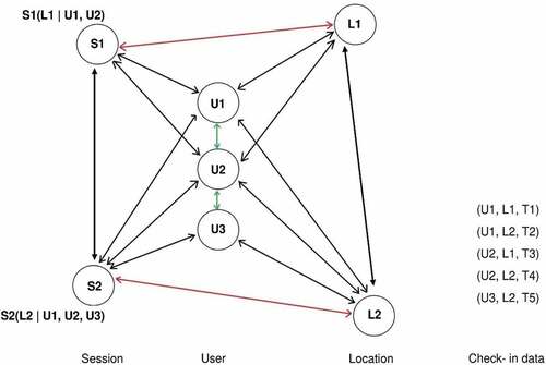
GHTG graph is defined as a pair $G=\left(V,E\right)$ with $V$ representing the set of nodes of the types User, Session and Location and $E$ representing the set of edges of the types user-user, user-location, user-session, location-location, location-user, session-session, session-user, location-session, and session-location. An edge $e=xy$ connects two nodes $x$ and $y$. GHTG

The edges in GHTG are created based on the following rules.

• If two users $u_1$ and $u_2$ are friends together, a user-user edge $e=u_1{u}_2$ is generated.

• We assumed that users are inclined to visit nearby locations and therefore, for each location $l$, its $k$ nearby locations are selected as $near=\left[l_1^{\prime },l_2^{\prime },\dots ,l_k^{\prime }\right]$. For each pair $l$ and $l_i^{\prime }\in near$, a location-location edge $e=l{l}_i^{\prime }$ is generated.

• If a user $u$ visits a location $l$ (check-in), a user-location edge $e=ul$ is generated.

• Consider $U_l^{tw}=\left[u_1,\dots ,u_m\right]$ as the list of all users that visited location $l$ at time window $tw$. If $m>1$, meaning that more than one user has visited $l$ at $tw$, a new Session node $s$ is generated. Having $s$, for each $u\in U_l^{tw}$ a user-session edge $e_1=us$ is created. Additionally, a Session-Location edge $e_2=sl$ is generated.

• Consider S_s=[s₁,…,s_Ʊ] as the list of Ʊ neighboring sessions of session $s$. For each $s{ }^{\mathrm{\prime }}\in S_s$, a new session-session edge $e=ss{ }^{\mathrm{\prime }}$ is generated. The Ʊ neighboring sessions of session $s$, are selected based on the distance of their respective location to the location of session $s$.

In the proposed graph, each edge type represents a subnet of the GHTG graph. Generally, the special characteristics of GHTG are as follows.

• The GHTG is a directed and weighted graph.

• The two edges of location-session and session-location are considered.

• Only the K nearest locations to each location node are used to create the location-location subnet, and establish a connection between them.

• In the same way, only the K nearest session to each session node are used to construct the session-session subnet.

3.2. Weighting and construction of transition probability matrix

Having GHTG, the next step is to generate a weight matrix, which includes the weight of the connections between each pair of nodes in the graph. The weights of the session-session, session-location, user-session, user-user, user-location, location-user, and location-location blocks are calculated using Equations (3(3) $w\left(s,s^{,}\right)=\left(1-\frac{dist\left(s,s^{,}\right)}{{\sum }_{\mathrm{\forall }s,s^{,}\in S}\left(dist\left(s,s^{,}\right)\right)}\right)+\left(1-\frac{\mathrm{\Delta }t\left(s,s^{,}\right)}{{\sum }_{\mathrm{\forall }s,s^{,}\in S}\left(\mathrm{\Delta }t\left(s,s^{,}\right)\right)}\right)$(3) ) to (9(9) $w\left(l,l^{,}\right)=\left(1-\frac{dist\left(l,l^{,}\right)}{{\sum }_{\mathrm{\forall }l,l^{,}\in L}\left(dist\left(l,l^{,}\right)\right)}\right)$(9) ), based on Kefalas et al. (Kefalas et al. 2018)’s study. Table S1 shows the list of all used symbols, notations, and descriptions.

(3) $w\left(s,s^{,}\right)=\left(1-\frac{dist\left(s,s^{,}\right)}{{\sum }_{\mathrm{\forall }s,s^{,}\in S}\left(dist\left(s,s^{,}\right)\right)}\right)+\left(1-\frac{\mathrm{\Delta }t\left(s,s^{,}\right)}{{\sum }_{\mathrm{\forall }s,s^{,}\in S}\left(\mathrm{\Delta }t\left(s,s^{,}\right)\right)}\right)$(3)

(4) $w(s,u)=\frac{1}{|U_s|}$(4)

(5) $w(u,s)=\frac{1}{|S_u|}$(5)

(6) $w(u,u^{\prime })=\frac{1}{|U_u|}$(6)

(7) $w\left(u,l\right)=\frac{n_{u,l}}{{\sum }_{\mathrm{\forall }l\in L}{n}_{u,l}}$(7)

(8) $w\left(l,u\right)=\frac{n_{l,u}}{{\sum }_{\mathrm{\forall }u\in U}{n}_{l,u}}$(8)

(9) $w\left(l,l^{,}\right)=\left(1-\frac{dist\left(l,l^{,}\right)}{{\sum }_{\mathrm{\forall }l,l^{,}\in L}\left(dist\left(l,l^{,}\right)\right)}\right)$(9)

In order to weight location-session and session-location edges, we used Equations (10(10) $\mathrm{w}(l,s)=\frac{1}{|S_l|}$(10) ) and (11(11) $\mathrm{w}(s,l)=\frac{1}{|L_s|}$(11) ), respectively.

(10) $\mathrm{w}(l,s)=\frac{1}{|S_l|}$(10)

(11) $\mathrm{w}(s,l)=\frac{1}{|L_s|}$(11)

In Equations (10(10) $\mathrm{w}(l,s)=\frac{1}{|S_l|}$(10) ) and (11(11) $\mathrm{w}(s,l)=\frac{1}{|L_s|}$(11) ), $|S_l|$ is the total number of sessions that a location $l$ has participated in and $|L_s|$ is the total number of locations that a session $s$ has participated in.

Using Equations (3(3) $w\left(s,s^{,}\right)=\left(1-\frac{dist\left(s,s^{,}\right)}{{\sum }_{\mathrm{\forall }s,s^{,}\in S}\left(dist\left(s,s^{,}\right)\right)}\right)+\left(1-\frac{\mathrm{\Delta }t\left(s,s^{,}\right)}{{\sum }_{\mathrm{\forall }s,s^{,}\in S}\left(\mathrm{\Delta }t\left(s,s^{,}\right)\right)}\right)$(3) ) to (11(11) $\mathrm{w}(s,l)=\frac{1}{|L_s|}$(11) ), we can calculate the weights of all the partitions of the graph and generate a weight adjacency matrix in the form of Fig. S3. This weight adjacency matrix represents the probability of transition between each pair of nodes in the graph. Therefore, we can say that by calculating the weight adjacency matrix, we have the transition probability matrix with nine partitions, including $SS,SU,SL,US,$ $UU,UL,LS,LU,\mathrm{a}\mathrm{n}\mathrm{d}LL$.

(12) $P=\left[\begin{array}{ccc}SS& SU& SL\\ US& UU& UL\\ LS& LU& LL\end{array}\right]$(12)

To normalize matrix $P$, the theorem proposed by Chu et al. (Chu and Guo 1998) is adopted, and the positive maximal eigenvalue and the positive maximal eigenvector (Equation (13))(13) $x=[x1,x2,\dots ,xn]$(13) of the matrix $P$ are calculated. Then a diagonal matrix based on the positive maximal eigenvector (Equation (14))(14) $D=\left[\begin{array}{ccc}{x}_1& \cdots & 0\\ ⋮& \ddots & ⋮\\ 0& \cdots & x_n\end{array}\right]$(14) is constructed.

(13) $x=[x1,x2,\dots ,xn]$(13)

(14) $D=\left[\begin{array}{ccc}{x}_1& \cdots & 0\\ ⋮& \ddots & ⋮\\ 0& \cdots & x_n\end{array}\right]$(14)

Using Equation (15)(15) $P^{\prime }=D^{-1}.q^{-1}.P\left(i,j\right).D$(15) , the transition probability matrix is converted to a stochastic matrix so that the sum of the values in each column equals to 1 (Chu and Guo 1998), where $q$ is the positive maximal eigenvalue and $P^{\prime }$ shows the normalized transition probability matrix.

(15) $P^{\prime }=D^{-1}.q^{-1}.P\left(i,j\right).D$(15)

3.3. User similarity calculation

Having the normalized transition probability matrix, $P^{\prime }$, the next step is to find the most similar users to the user $u$, using ERWR. The users’ similarity matrix in ERWR is calculated using Equation (16)$\begin{array}{rl}& S^{(UU)t+1}=(1+\alpha )\cdot \left(\left(\frac{\gamma }{2}\cdot US\right)\cdot \left(\frac{\omega }{2}\cdot SL\right)\cdot \left(\xi \cdot LL\right)\cdot \left(\frac{\epsilon }{2}\cdot LU\right)+\left(\delta \cdot UU\right)+\left(\frac{\epsilon }{2}\cdot UL\right)\cdot \left(\frac{\omega }{2}\cdot LS\right)\cdot \left(\beta \cdot SS\right)\cdot \left(\frac{\gamma }{2}\cdot US\right)\right)\\ & \cdot S^{(UU)t}+\alpha \cdot I\end{array}$ as an extension to the RWRS algorithm (see Section 1.3) by incorporating the two new subnets of LS and SL.

$\begin{array}{rl}& S^{(UU)t+1}=(1+\alpha )\cdot \left(\left(\frac{\gamma }{2}\cdot US\right)\cdot \left(\frac{\omega }{2}\cdot SL\right)\cdot \left(\xi \cdot LL\right)\cdot \left(\frac{\epsilon }{2}\cdot LU\right)+\left(\delta \cdot UU\right)+\left(\frac{\epsilon }{2}\cdot UL\right)\cdot \left(\frac{\omega }{2}\cdot LS\right)\cdot \left(\beta \cdot SS\right)\cdot \left(\frac{\gamma }{2}\cdot US\right)\right)\\ & \cdot S^{(UU)t}+\alpha \cdot I\end{array}$

In Equation (16)$\begin{array}{rl}& S^{(UU)t+1}=(1+\alpha )\cdot \left(\left(\frac{\gamma }{2}\cdot US\right)\cdot \left(\frac{\omega }{2}\cdot SL\right)\cdot \left(\xi \cdot LL\right)\cdot \left(\frac{\epsilon }{2}\cdot LU\right)+\left(\delta \cdot UU\right)+\left(\frac{\epsilon }{2}\cdot UL\right)\cdot \left(\frac{\omega }{2}\cdot LS\right)\cdot \left(\beta \cdot SS\right)\cdot \left(\frac{\gamma }{2}\cdot US\right)\right)\\ & \cdot S^{(UU)t}+\alpha \cdot I\end{array}$, $US$, $SL$, $LL$, $LU$, $UU$, $UL$, $LS$, $SS$, and $US$ are the partitions of $P^{\prime }$. ${S^{\left(UU\right)}}^t$and ${S^{\left(UU\right)}}^{t+1}$ are the $u\times u$ user similarity matrices at steps $t$ and $t+1$, respectively, representing the similarity between all pairs of users. The coefficients $\beta ,\gamma ,\delta ,\omega ,\xi ,\epsilon$, all range between 0 and 1, control the contribution of each subnet of GHTG in the random walk process. Also, $\alpha ,$ which is the restarting probability of the random walk algorithm, was set to 0.8. ${S^{\left(UU\right)}}^{t+1}$ also is calculated iteratively as the RWR algorithm (Section 2.2).

3.4. Time-aware location recommendation

To recommend favorable locations to the active user $u$ at a specific time$t$, $K$ most similar users are selected from the user similarity matrix ($S^{\left(UU\right)}$, calculated iteratively using Equation (16)$\begin{array}{rl}& S^{(UU)t+1}=(1+\alpha )\cdot \left(\left(\frac{\gamma }{2}\cdot US\right)\cdot \left(\frac{\omega }{2}\cdot SL\right)\cdot \left(\xi \cdot LL\right)\cdot \left(\frac{\epsilon }{2}\cdot LU\right)+\left(\delta \cdot UU\right)+\left(\frac{\epsilon }{2}\cdot UL\right)\cdot \left(\frac{\omega }{2}\cdot LS\right)\cdot \left(\beta \cdot SS\right)\cdot \left(\frac{\gamma }{2}\cdot US\right)\right)\\ & \cdot S^{(UU)t}+\alpha \cdot I\end{array}$. For each location $l$, the frequency of $l$ being visited by $u$ at a specific timestamp (i.e. $r_{u_i,t,l}$) is computed based on the user’s check-in history. All existing locations in the dataset are rated using the calculated frequencies and the ratings of $K$ similar user afterward. Finally, a list of $N$ top-rated locations is recommended to the target user using Equation (17)(17) ${r^{\wedge }}_{u,t,l}=\frac{{\sum }_{i=1}^n{S}_i\cdot {r_u}_{{ }_i,t,l}}{{\sum }_{i=1}^n{S}_i}$(17) .

(17) ${r^{\wedge }}_{u,t,l}=\frac{{\sum }_{i=1}^n{S}_i\cdot {r_u}_{{ }_i,t,l}}{{\sum }_{i=1}^n{S}_i}$(17)

In Equation (17)(17) ${r^{\wedge }}_{u,t,l}=\frac{{\sum }_{i=1}^n{S}_i\cdot {r_u}_{{ }_i,t,l}}{{\sum }_{i=1}^n{S}_i}$(17) , $s_i$, which is the similarity values of $n$ most similar users to the target user, was set to 10 in this study.

4. Experimental evaluation

4.1. Data preparation and setting

In this study, the experiments were conducted on the two real-world datasets, namely Gowalla and Weeplaces.¹ Gowalla dataset was gathered from 246 real users who lived in Germany between September 2010 and November 2010. It contains 34051 check-ins on 7746 locations. Also, the Weeplaces dataset contains 570 users, 3025 locations, and 12815 check-ins that were recorded in Spain during April 2009 and June 2011. Further information regarding the datasets, including the number of users, locations, check-in records, the average number of check-in per user, denoted as$\mathrm{A}\mathrm{V}{\mathrm{G}}_{\mathrm{u}}$, and the average check-in per location denoted as $\mathrm{A}\mathrm{V}{\mathrm{G}}_{\mathrm{l}}$ are presented in Table 2. The datasets did not include any information about the ratings that users would assign to the locations.

Table 2. Datasets specification.

Dataset	# Users	#Locations	#Check-ins	$\mathbf{A}\mathbf{V}{\mathbf{G}}_{\mathbf{u}}$	$\mathbf{A}\mathbf{V}{\mathbf{G}}_{\mathbf{l}}$
Weeplaces	570	3025	12815	22.48	4.24
Gowalla	246	7746	34051	138.42	4.39

Also, Table 3 shows the information about the session nodes for each of the datasets separately. The session nodes are created based on the hours of the day (e.g. 3–6 AM, 3–6 PM, etc.), and we ignored factors such as weekdays and holidays. To evaluate the effect of the length of the time window in the POI recommendation process, we extracted the session nodes from the available datasets in 6-hour, 12-hour, and 24-hour time intervals. The distributions of visited locations in both datasets are presented in Fig. S4, as well.

Table 3. Session node extraction at different time windows.

Dataset	6-hour	12-hour	24-hour
Weeplaces	76	111	120
Gowalla	851	988	1520

The recommendation model was trained, and the process of recommendation was done only using the test data. Then, $N$ POIs with the highest ratings were recommended to the user. Finally, the results of the recommendation were derived from the model, and the expected results in the test data were compared to evaluate the quality and precision of the recommendation. This experiment was repeated 50 times so that in each iteration, 80% of the data was randomly considered as train and the remaining 20% as test.

4.2. Evaluation metrics

To evaluate the effect of the proposed GHTG-ERWR algorithm on location recommendation for each user, we examined how many of the visited POIs in the test data have been discovered by the model. To do so, we used standard evaluation metrics of Precision, Recall (Kefalas and Manolopoulos 2017), and F-score (Kefalas et al. 2018) via Equations (18(18) $Precision=\frac{\mathrm{\#}\left(Relevant\cap Retrieved\right)}{\mathrm{\#}Retrieved}$(18) ), (19(19) $Recall=\frac{\mathrm{\#}\left(Relevant\cap Retrieved\right)}{\mathrm{\#}Relevant}$(19) ), and (20(20) $F-Score=2\ast \frac{\mathrm{P}recision\ast Recall}{Precision+Recall}$(20) ), respectively.

(18) $Precision=\frac{\mathrm{\#}\left(Relevant\cap Retrieved\right)}{\mathrm{\#}Retrieved}$(18)

(19) $Recall=\frac{\mathrm{\#}\left(Relevant\cap Retrieved\right)}{\mathrm{\#}Relevant}$(19)

Precision is the ratio of the number of relevant locations in the top-N list to the number of retrieved locations, and Recall is the ratio of the number of relevant locations in the top-N list to the total number of relevant locations. The relevant locations are defined as the locations in the test dataset associated with the target user. In contrast, the retrieved locations are the top-N locations suggested to the target user. F-score or F1 is a metric that combines both Precision and Recall and measures the recommendation algorithm’s accuracy.

(20) $F-Score=2\ast \frac{\mathrm{P}recision\ast Recall}{Precision+Recall}$(20)

4.3. Tuning

In order to achieve the best performance, we calibrated the parameters of GHTG-ERWR, including β,γ,δ,ω,ξ,ϵ,k, and Ʊ. In the first step, the six parameters of $\beta ,\gamma ,\delta ,\omega ,and\epsilon$ were calibrated through investigating the impact of their related sub-matrix on location recommendation performance. We evaluated the performance of the proposed algorithm on available datasets by changing each parameter in the range of 0.2 to 0.8 while keeping the other parameters constant.

Then, we examined the effect of the nearest session nodes, Ʊ, on the performance of location recommendation. Finally, in the third step, the impact of parameter $k$, the number of nearest locations, were explored.

The results of the first step of parameter tuning, shown in Fig. S5 (a) and Fig. S5 (b), revealed that the $\gamma$ and $\beta$ coefficients had the most significant effect on location recommendation in the Weeplaces and Gowalla datasets. In other words, the contributions of sub-matrices session-user, user-session, and session-session in location recommendation were higher than other sub-matrices. Additionally, as shown in Fig. S5 (c) and Fig. S5 (d), for Ʊ = 40 and Ʊ = 500, the proposed algorithm had better performance for Weeplaces and Gowalla datasets, respectively. Nevertheless, in general, this parameter did not significantly change the accuracy of the outputs. Considering the $k$ parameter, it is expected that the lower the value of $k$, the more accurate the recommendation, but the results of adjusting this parameter showed that changing this parameter did not have a significant effect on the two available datasets. This indicates that interests were more important than distance for the users, and users chose a place to visit according to their preferences, not based on the distance or proximity of that place. Nonetheless, as shown in Fig. S5 (e), the algorithm performed better in k = 500 and k = 700 for Weeplaces and Gowalla, respectively.

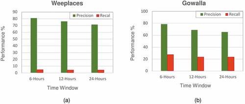
The lengths of the time window (TW) in the recommender process can significantly affect the way we capture the users’ behavioral patterns. Therefore, we examined our GHTG-ERWR algorithm for the three-time windows of 6, 12, and 24 hours in terms of Precision and Recall. As depicted in Figure 2, the highest Precision was obtained for the 6-hour window by 80.95% and 78.54% for Weeplaces and Gowalla datasets, respectively.

Figure 2. Performance of GHTG-ERWR algorithm in locations recommendation at different time windows for (a) Weeplaces and (b) Gowalla datasets.

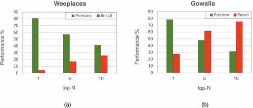
Additionally, Figure 3 reports the Precision and Recall for the top-N locations ($N=\left[1,5,10\right]$) to demonstrate the effect of the number of recommended locations. The results of the Weeplaces datasets reveal a steady decline in the value of Precision from 71.43% for $N=1$ to 41.43% for $N=10$. Nonetheless, this dataset has experienced a remarkable rise in the value of Recall from 4.05 to 25.68 for $N=1$ and $N=10$, respectively. For the Gowalla dataset, the value of Precision decreases by about 46.76% from $N=1$ to $N=10,$ and the value of Recall increases to approximately 47.78%. As shown in Figure 3, the value of Recall is higher than the value of Precision in $N=5$ and $N=10$ for the Gowalla dataset, which could be related to the limited number of locations in the test dataset. It seems that the number of locations in the test dataset affected Recall calculation (Equation (19)(19) $Recall=\frac{\mathrm{\#}\left(Relevant\cap Retrieved\right)}{\mathrm{\#}Relevant}$(19) ), while this issue was not effective on Precision.

Figure 3. Performance of GHTG-ERWR algorithm in different number of recommended locations for (a) Weeplaces and (b) Gowalla datasets.

The negative correlation between the length of the time window and the performance proves that increasing the size of the time window for extracting the session node decreases the sensitivity of the recommendation to the time. Besides, the results confirmed that the same relation exists between the number of recommended locations and performance. Remarkably, these correlations express the high performance of the algorithm and show that the priorities computed by the algorithm are incredibly similar to the real priorities of the users.

4.4. Comparison

To further discuss the performance of GHTG-ERWR, we compared the results with those of RWR-HST, as the newest and most advanced graph-based POI recommendation algorithm. It should be noted that the superiority of RWR-HST over previous graph-based algorithms of STG, GTAG-BPP, and fast-katz had been proven before.

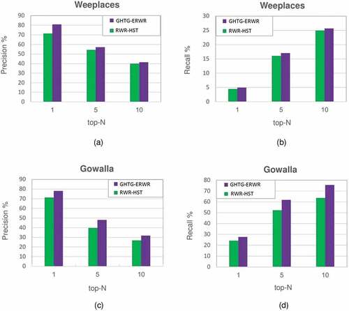
As shown in Figure 4(a) and (c), GHTG-ERWR outperforms RWR-HST by 9.52% and 7.31% increase in the value of Precision for the top-1 and 4.99% and 1.43% increase for the top-10 suggested locations for Weeplaces and Gowalla datasets, respectively. Figure 4(b) and (d) also show a rise in the value of Recall to about 0.48% and 3.51% for the top-1 and 0.75% and 11.88% for the top-10 recommended locations for Weeplaces and Gowalla datasets, respectively.

Figure 4. Comparison of GHTG-ERWR and RWR-HST algorithms for the Weeplaces datasets (a) Precision of top-N and (b) Recall of top-N. For the Gowalla dataset (c) Precision of top-N, (d) Recall of top-n.

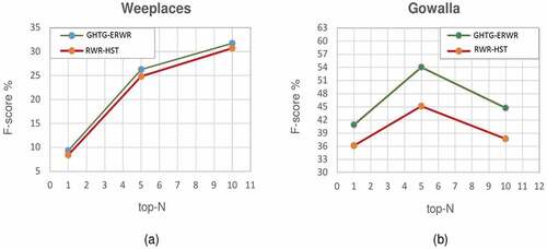
Besides, comparing the performance of GHTG-ERWR with RWR-HST in terms of F-score (Figure 5) shows an improvement of about 8.88% and 1.44% for recommending the top-5 locations for the Gowalla and Weeplaces datasets, respectively. Notably, the value of F-score for the top-5 suggested locations is higher than the values for the top-1 and the top-10, for both GHTG-ERWR and RWR-HST algorithms.

Figure 5. Comparison of the performance of GHTG-ERWR and RWR-HST algorithms in term of F-score for (a) Weeplaces and (b) Gowalla.

The improvements in the performance of the GHTG-ERWR algorithm roots back to the changes in the graph structure. In fact, adding the session-location and location-session edges in this study has led to the modeling of shared spatio-temporal preferences of users as auxiliary information in the graph. This auxiliary information specifies which users have visited a particular location at a specific time window and shows the similar interests of those users over that time window. Therefore, GHTG-ERWR overcomes the shortcomings of the RWR-HST algorithm and provides a more efficient location recommendation by applying this auxiliary information to the users’ similarity calculation.

A quick comparison between the average number of check-ins per user and the number of existing locations reveals that each user has visited only a few locations in each dataset, which means that we are dealing with severe sparsity in these datasets. As shown in Table 2, the average number of check-ins per user ($AV{G}_u$) for Gowalla and Weeplaces datasets are 22.48 and 138.42, respectively. Additionally, the number of locations in these datasets is 3025 for Gowalla and 7746 for Weeplaces. However, the proposed GHTG-ERWR algorithm improves the recommendation performance and handles this sparsity more stably in comparison to RWR-HST.

Finally, the findings of this study highlight a significant difference between the results of Gowalla and Weeplaces datasets. As shown in Fig. S6, GHTG-ERWR performs better on the Gowalla dataset in comparison to the Weeplaces dataset. It seems that the average number of sessions per user and the value of $AV{G}_u$ are the main reasons for this inconstancy. As shown in Tables 2 and 3, the average sessions per user of Gowalla and Weeplaces datasets for a 6-hour time window is 3.46 and 0.13, respectively. This means that each user in the Gowalla dataset participates in almost three sessions, and therefore finding co-locations among users in the Gowalla dataset is more accessible than the Weeplaces dataset. Moreover, the value of $AV{G}_u$ in Gowalla is higher than the Weeplaces dataset, so data sparsity in Gowalla is less than the Weeplaces dataset, and $UL$ and $LU$ sub-matrices are less sparse.

5. Conclusion

This paper presented a graph-based location recommendation method called GHTG-ERWR, as an extension to RWR-HST, to suggest POIs to users at preferred times based on their previous activities and preferences. In addition to considering the geographical effects and dynamics of users’ interests over time and space, the proposed method models shared spatio-temporal preferences of users as a new factor in the recommendation process. We also applied the ERWR algorithm to accurately calculate the similarity between all users’ pairs from the GHTG graph. The experimental results on the two real-world datasets proved that utilizing this new factor in the proposed algorithm can significantly increase recommendation accuracy and performance compared to the RWR-HST algorithm.

Several approaches can be perceived to develop further and improve the accuracy of GHTG-ERWR. Considering both temporal and spatial distances in calculating the weight of session-session edges may influence the recommendation’s accuracy. Incorporating the information derived from different location categories can improve the quality of the recommendation process. Additionally, accounting for the sequence of check-ins in the graph construction phase could improve the algorithm’s performance. Utilization and assessment of other graph-based recommendation algorithms, such as SimRank, to calculate the user similarity in GHTG can be considered future work of this study. A combination of clustering techniques with the graph-based mechanism for POI recommendation is also an open area for future studies. Last but not least, comparing the output of this graph-based POI recommendation approach with other classes of POI recommendation that work based on CF and CB could provide valuable input for further improvements.

Disclosure statement

No potential conflict of interest was reported by the author(s).

Supplementary material

Supplemental data for this article can be accessed here.

Notes

1. http://www.yongliu.org/datasets/.

References

- Broccolo, D., et al., 2012. Generating suggestions for queries in the long tail with an inverted index. Information Processing & Management, 48 (2), 326–339. doi:10.1016/j.ipm.2011.07.005
- Chen, J., et al., 2016. Effective successive POI recommendation inferred with individual behavior and group preference. Neurocomputing, 210, 174–184. doi:10.1016/j.neucom.2015.10.146
- Chu, M.T. and Guo, Q., 1998. A numerical method for the inverse stochastic spectrum problem. SIAM Journal on Matrix Analysis and Applications, 19 (4), 1027–1039. doi:10.1137/S0895479896292418
- Ding, Y. and Li, X., 2005. Time weight collaborative filtering. Paper presented at the proceedings of the 14th ACM international conference on information and knowledge management. Bremen, Germany.
- Gao, H., et al., 2013. Exploring temporal effects for location recommendation on location-based social networks. Paper presented at the proceedings of the 7th ACM conference on recommender systems. Hong Kong, China.
- Gao, H., Tang, J., and Liu, H., 2012. gSCorr: modeling geo-social correlations for new check-ins on location-based social networks. Paper presented at the proceedings of the 21st ACM international conference on information and knowledge management. Maui Hawaii, USA.
- Guo, T., et al., 2018. Differentially private graph-link analysis based social recommendation. Information Sciences, 463, 214–226. doi:10.1016/j.ins.2018.06.054
- Kant, S. and Mahara, T., 2018. Nearest biclusters collaborative filtering framework with fusion. Journal of Computational Science, 25, 204–212. doi:10.1016/j.jocs.2017.03.018
- Kefalas, P. and Manolopoulos, Y., 2017. A time-aware spatio-textual recommender system. Expert Systems with Applications, 78, 396–406. doi:10.1016/j.eswa.2017.01.060
- Kefalas, P., Symeonidis, P., and Manolopoulos, Y., 2018. Recommendations based on a heterogeneous spatio-temporal social network. World Wide Web, 21 (2), 345–371. doi:10.1007/s11280-017-0454-0
- Konstas, I., Stathopoulos, V., and Jose, J.M., 2009. On social networks and collaborative recommendation. Paper presented at the proceedings of the 32nd international ACM SIGIR conference on research and development in information retrieval. Boston, MA.
- Koren, Y., 2009. Collaborative filtering with temporal dynamics. Paper presented at the proceedings of the 15th ACM SIGKDD international conference on knowledge discovery and data mining. Paris France.
- Lee, S., et al., 2011. Random walk based entity ranking on graph for multidimensional recommendation. Paper presented at the proceedings of the fifth ACM conference on recommender systems. Chicago, IL.
- Li, Y., et al., 2014. Spatial-aware interest group queries in location-based social networks. Data & Knowledge Engineering, 92, 20–38. doi:10.1016/j.datak.2014.06.001
- Litou, I., Boutsis, I., and Kalogeraki, V., 2017. Efficient techniques for time-constrained information dissemination using location-based social networks. Information Systems, 64, 321–349. doi:10.1016/j.is.2015.12.002
- Liu, S., et al., 2019. Evolving graph construction for successive recommendation in event-based social networks. Future Generation Computer Systems,96, 502–551.
- Lovász, L., 1993. Random walks on graphs: a survey. Combinatorics, Paul erdos is eighty, 2 (1), 1–46.
- Lu, J. and Wang, H., 2014. Variance reduction in large graph sampling. Information Processing & Management, 50 (3), 476–491. doi:10.1016/j.ipm.2014.02.003
- Luo, L., et al., 2019. Personalized recommendation by matrix co-factorization with tags and time information. Expert Systems with Applications, 119, 311–321. doi:10.1016/j.eswa.2018.11.003
- Lyu, Y., et al., 2019. iMCRec: a Multi-Criteria Framework for Personalized Point-of-Interest Recommendations. Information Sciences, 483, 294–312.
- Melville, P., Mooney, R.J., and Nagarajan, R., 2002. Content-boosted collaborative filtering for improved recommendations. Aaai/iaai, 23, 187–192.
- Musto, C., et al., 2017. Introducing linked open data in graph-based recommender systems. Information Processing & Management, 53 (2), 405–435. doi:10.1016/j.ipm.2016.12.003
- Najafabadi, M.K., Mohamed, A., and Onn, C.W., 2019. An impact of time and item influencer in collaborative filtering recommendations using graph-based model. Information Processing & Management, 56 (3), 526–540. doi:10.1016/j.ipm.2018.12.007
- Niu, J., et al., 2016. FUIR: fusing user and item information to deal with data sparsity by using side information in recommendation systems. Journal of Network and Computer Applications, 70, 41–50. doi:10.1016/j.jnca.2016.05.006
- Noulas, A., et al., 2012. A random walk around the city: new venue recommendation in location-based social networks. Paper presented at the privacy, security, risk and trust (PASSAT), 2012 international conference on and 2012 international confernece on social computing (socialcom). Amsterdam, Netherlands.
- Nzeko’O, A.J.N., Tchuente, M., and Latapy, M., 2017. Time weight content-based extensions of temporal graphs for personalized recommendation. Paper presented at the WEBIST 2017-13th international conference on web information systems and technologies. Porto, Portugal.
- Orso, V., et al., 2017. Overlaying social information: the effects on users’ search and information-selection behavior. Information Processing & Management, 53 (6), 1269–1286. doi:10.1016/j.ipm.2017.06.001
- Pongnumkul, S. and Motohashi, K., 2015. Random walk-based recommendation with restart using social information and bayesian transition matrices. International Journal of Computer Applications, 114 (9), 32–38. doi:10.5120/20009-1960
- Popescul, A., Pennock, D.M., and Lawrence, S., 2001. Probabilistic models for unified collaborative and content-based recommendation in sparse-data environments. Paper presented at the proceedings of the seventeenth conference on uncertainty in artificial intelligence. San Francisco, CA: USA.
- Qi, L., et al., 2019. Time-aware distributed service recommendation with privacy-preservation. Information Sciences, 480, 354–364. doi:10.1016/j.ins.2018.11.030
- Rafailidis, D., Kefalas, P., and Manolopoulos, Y., 2017. Preference dynamics with multimodal user-item interactions in social media recommendation. Expert Systems with Applications, 74, 11–18. doi:10.1016/j.eswa.2017.01.005
- Ren, X., et al., 2017. Context-aware probabilistic matrix factorization modeling for point-of-interest recommendation. Neurocomputing, 241, 38–55. doi:10.1016/j.neucom.2017.02.005
- Si, Y., Zhang, F., and Liu, W., 2017. CTF-ARA: an adaptive method for POI recommendation based on check-in and temporal features. Knowledge-Based Systems, 128, 59–70. doi:10.1016/j.knosys.2017.04.013
- Si, Y., Zhang, F., and Liu, W., 2019. An adaptive point-of-interest recommendation method for location-based social networks based on user activity and spatial features. Knowledge-Based Systems, 163, 267–282. doi:10.1016/j.knosys.2018.08.031
- Sun, G., et al., 2019. Towards privacy preservation for “check-in” services in location-based social networks. Information Sciences, 481, 616–634. doi:10.1016/j.ins.2019.01.008
- Sun, Y., et al., 2015. Location information disclosure in location-based social network services: privacy calculus, benefit structure, and gender differences. Computers in Human Behavior, 52, 278–292. doi:10.1016/j.chb.2015.06.006
- Tong, H., Faloutsos, C., and Pan, J.-Y., 2006. Fast random walk with restart and its applications. Paper presented at the sixth international conference on data mining (ICDM’06). Hong Kong, China.
- Valverde-Rebaza, J.C., et al., 2018. The role of location and social strength for friendship prediction in location-based social networks. Information Processing & Management, 54 (4), 475–489. doi:10.1016/j.ipm.2018.02.004
- Wang, W., et al., 2017. ST-SAGE: a spatial-temporal sparse additive generative model for spatial item recommendation. ACM Transactions on Intelligent Systems and Technology (TIST), 8 (3), 48.
- Xia, B., et al., 2017. Vrer: context-based venue recommendation using embedded space ranking SVM in location-based social network. Expert Systems with Applications, 83, 18–29. doi:10.1016/j.eswa.2017.04.020
- Xiang, L., et al., 2010. Temporal recommendation on graphs via long-and short-term preference fusion. Paper presented at the proceedings of the 16th ACM SIGKDD international conference on knowledge discovery and data mining. Washington DC.
- Xie, M., et al., 2016. Learning graph-based POI embedding for location-based recommendation. Paper presented at the proceedings of the 25th ACM international on conference on information and knowledge management. Indianapolis, USA.
- Yang, X., et al., 2014. A survey of collaborative filtering based social recommender systems. Computer Communications, 41, 1–10. doi:10.1016/j.comcom.2013.06.009
- Yang, Y., Hooshyar, D., and Lim, H.S., 2019. GPS: factorized group preference-based similarity models for sparse sequential recommendation. Information Sciences, 481, 394–411. doi:10.1016/j.ins.2018.12.053
- Ying, Y., Chen, L., and Chen, G., 2017. A temporal-aware POI recommendation system using context-aware tensor decomposition and weighted HITS. Neurocomputing, 242, 195–205. doi:10.1016/j.neucom.2017.02.067
- Yu, C., et al., 2017a. Using check-in features to partition locations for individual users in location based social network. Information Fusion, 37, 86–97. doi:10.1016/j.inffus.2017.01.006
- Yu, J., Shen, Y., and Yang, Z., 2014. Topic-STG: extending the session-based temporal graph approach for personalized tweet recommendation. Paper presented at the proceedings of the 23rd international conference on world wide web. Seoul, Republic of Korea.
- Yu, L., et al., 2017b. TIIREC: a tensor approach for tag-driven item recommendation with sparse user generated content. Information Sciences, 411, 122–135. doi:10.1016/j.ins.2017.05.025
- Yuan, Q., Cong, G., and Sun, A., 2014. Graph-based point-of-interest recommendation with geographical and temporal influences. Paper presented at the proceedings of the 23rd ACM international conference on conference on information and knowledge management. Shanghai, China.
- Zhang, C., et al., 2014. Latent factor transition for dynamic collaborative filtering. Paper presented at the proceedings of the 2014 SIAM international conference on data mining. Philadelphia, Pennsylvania.
- Zhang, S. and Cheng, H., 2018, Exploiting Context Graph Attention for POI Recommendation in Location-Based Social Networks. In: Pei J., Manolopoulos Y., Sadiq S., Li J. (eds) Database Systems for Advanced Applications. DASFAA 2018. Lecture Notes in Computer Science, vol 10827. Springer, Cham.
- Zhao, S., et al., 2016. STELLAR: spatial-temporal latent ranking for successive point-of-interest recommendation. Paper presented at the thirtieth AAAI conference on artificial intelligence. Phoenix, Arizona USA
- Zhou, W. and Han, W., 2019. Personalized recommendation via user preference matching. Information Processing & Management, 56 (3), 955–968. doi:10.1016/j.ipm.2019.02.002