Design, construction, and evaluation of energy-harvesting asphalt pavement systems

Abstract

Energy-harvesting pavements, one of which is the Hydronic Asphalt Pavement (HAP) system, have been proven to be both more durable and sustainable than conventional pavement systems. A HAP consists of a system of connected pipes embedded within the asphalt pavement which function to extract or reject heat from/into the pavement via a circulating fluid. Three large-scale systems were designed and constructed in the field: a control section, a regular HAP section, and a section containing a HAP coupled to a horizontal ground heat exchanger (GCHAP). The field data showed that neither the HAP section nor the GCHAP section were able to substantially decrease the pavement surface temperature. However, both GCHAP and HAP were able to decrease the asphalt temperature at a depth of 2.5 cm below the surface by a magnitude of around 10°C. Another key finding of this study shows that increasing the conductivity of a flexible pavement asphalt layer, rather than increasing the conductivity of the embedded pipes, significantly enhances the effectiveness of the HAP system.

Keywords:

• hydronic
• HAP
• energy-harvesting
• geothermal
• asphalt
• pavement

1. Introduction

Roads provide nations and individuals the improved ability of transporting goods, people, and information. The Federal Highway Administration has reported as much as 6.5 million kilometres of paved public roads in the United States (FHWA, 2004), estimated to value a tremendous 1.75 trillion USD (Sorenson, 2006). This huge investment merits employing long-term strategies that contribute to the pavement’s performance, whether through extending the pavement’s life by decreasing distresses such as cracking and permanent deformation or improving the road safety by decreasing accidents due to ice and snow accumulation during winter. Lately, the concept of Hydronic Asphalt Pavements (HAPs) has emerged as an alternative pavement system that is both durable and sustainable. HAP systems consist of a series of pipes embedded within the asphalt pavement which function to extract or reject heat from/into the pavement via a circulating fluid. The purpose of such a system can be any of the following: snow-melting and deicing, cooling the pavement, and/or energy extraction and harvesting.

By circulating a cold fluid through the HAP in summer, the system is able to decrease the pavement’s surface temperature which enhances its resistance to permanent deformation. This also leads to creating a more eco-friendly environment by mitigating the Urban Heat Island effect (UHI), a phenomenon known to directly cause urban areas to be several degrees warmer than the surrounding regions. In literature, a HAP system functioning in a summer setting is sometimes referred to as an Asphalt Solar Collector (ASC) (Bobes-Jesus, Pascual-Muñoz, Castro-Fresno, & Rodriguez-Hernandez, 2013). Alternatively, by circulating a hot fluid in winter, the system ensures snow-melting and deicing – thereby relieving the pavement from any damage incurred by spraying chemicals or employing mechanical methods – while also allowing safe passage for pedestrians and vehicles.

The vast majority of studies found in recent literature on this topic are limited to small-scale experimental tests and numerical simulations of hydronic systems utilising pipes or other means including porous layers (Asfour, Bernardin, Toussaint, & Piau, 2016). Only a handful of studies addressed the issues associated with large-scale implementation of the systems (Boyd, 2003; Carder, Barker, Hewitt, Ritter, & Kiff, 2008; Siebert & Zacharakis, 2010; Zwarycz, 2002). However, most of these large-scale systems are implemented in rigid pavements and would involve large amounts of resources to operate (vertical ground source heat exchangers, external heat sources, insulation, etc.). Large-scale HAP systems in flexible pavements could exhibit a behaviour different from that of small-scale lab tests conducted under controlled conditions for various reasons including, but not limited to, the heterogeneity of the asphalt, high construction temperatures and the employment of heavy equipment, and the involvement of contractors and numerous workers that might introduce variability unaccounted for in small-scale tests. It is also noteworthy that the HAP’s winter functionality has been less studied in the literature, and only few works have investigated how to optimise such systems (Eggen & Vangsnes, 2005; Eugster, 2007; Ho, Shan, Du, & Ishaku, 2015; Lund, 1999; Minsk, 1999). Winter functionality generally necessitates employing an external source of energy, but current research is being conducted to investigate whether geothermal energy sources can be utilised.

Since previous work has established the conceptual feasibility of the HAP system for flexible pavements in small-scale laboratory tests (Dakessian et al., 2016; Mallick, Chen, & Bhowmick, 2009; Pan, Wu, Xiao, & Liu, 2015), it has become essential to study the performance and behaviour of the system on a large-scale section subjected to realistic field conditions. Given the complex construction process of the HAP and the associated uncertainties, it is thus paramount to ensure that the proposed system is constructible and economical on large-scale before embarking with performance and life cycle cost assessment studies.

2. Objectives and scope

The main objective of this study is to design, construct, and evaluate energy-harvesting pavement systems such as HAP on a relatively large-scale setting. The incorporation of a geothermal energy component within a HAP system is also investigated by constructing another HAP system coupled to a horizontal heat exchanger embedded in the road’s subgrade.

To achieve the above objectives, the scope includes development of a numerical thermal model to study the sensitivity of the HAP system to different thermo-physical and geometrical parameters. This model is then used to predict the thermal behaviour of the system by running large-scale numerical simulations that are deemed critical in the design procedure. Constructability is studied by conducting lab tests and a pilot study on a pavement system with a reduced scale. The reduced scale study provides preliminary insight into the limitations and constraints that could prevail in the large-scale construction.

Finally, a large-scale construction of three pavement sections is executed: (1) HAP section, (2) HAP coupled to a piping network for geothermal energy extraction in the soil; this system will be henceforth called Ground-Coupled Hydronic Asphalt Pavement (GCHAP), and (3) a control section. The three systems are then evaluated based on their capability of decreasing pavement temperature compared to that of the control and consequent reduction in high-temperature distresses such as asphalt rutting.

3. Background

The dark colour of asphalt mixtures provides the asphalt surface layer of flexible pavements with better energy absorptivity due to the low reflectance of solar light wavelengths, leading to high surface temperatures that can reach up to 70°C and higher in summer (Pan et al., 2015). The temperature difference between the asphalt pavement and the circulating fluid, in the case of HAP, initiates a heat transfer process that cools the pavement.

Given the viscoelastic behaviour of asphalt concrete, layer properties vary significantly with temperature. Up until 1987, studies for surface layer temperature prediction revolved around empirical relations that were only applicable to specific conditions and locations (Barber, 1957; Christison & Anderson, 1972; Thompson, Dempsey, Hill, & Vogel, 1987). In the late 1990s, the introduction of the finite element method (FEM) and the finite difference method (FDM) enabled modelling of complex physical systems, such as the heat transfer processes and its impact on temperature distribution in the pavement (Hermansson, 2004; Kassem, Chehab, & Saad, 2015; Solaimanian & Kennedy, 1993; Timm, Voller, Lee, & Harvey, 2001; Yavuzturk, Ksaibati, & Chiasson, 2005). Table 1 summarises the results of many studies conducted to better understand the mechanisms involved in hydronic systems and to optimise the design of such systems.

Table 1. Studies on the various parameters involved in the design of HAPs.

Reference	Property	Study/Outcome
Abdel-Khalik (1976)	Pipe Configuration	Predicted the variation of fluid temperature in segments of serpentine configuration with arbitrary geometry and number of bends.
Chen, Bhowmick, and Mallick (2009)	Pipe Configuration	A serpentine configuration allows higher outlet water temperatures.
Chiou (1982)	Flow	The efficiency of the system can deteriorate anywhere between 2% and 20% due to flow non-uniformity.
Dakessian et al. (2016)	Pipe Configuration	A one reservoir looping configuration achieves lower efficiency due to the constantly decreasing temperature differential between the inflow and outflow water as opposed to the single pass system.
Deeb et al. (2013)	Pipe Diameter and Flow	The larger the diameter, the greater the decrease in surface temperature. For a constant flow, the larger the diameter pipe, the smaller the decrease in surface temperature.
Gui, Phelan, Kaloush, and Golden (2007)	Thermal Conductivity	The average maximum temperature decreases with increasing conductivity. The minimum surface temperature increases with conductivity.
	Volumetric Heat Capacity	The maximum temperature decreases while the minimum temperature increases with increasing volumetric heat capacity.
	Thermal Diffusivity	The average maximum surface temperature reduces while the minimum temperature increases with increasing diffusivity.
	Albedo	The higher the albedo, the lower the pavement maximum and minimum temperatures. The maximum temperature is more sensitive to albedo.
	Emissivity	The maximum and minimum surface temperatures decrease with increasing emissivity.
Mallick et al. (2009)	Thermal Conductivity	Aggregates with higher thermal conductivity such as quartzite increase the difference between incoming and outgoing water by 100% as compared to using limestone aggregates.
	Albedo	The lower the albedo, the higher the difference between incoming and outgoing water.
	Pipe Spacing	The fluid carrying pipes must be placed at a minimum spacing to avoid “cool” spot formation.
Shaopeng et al. (2011)	Flow	The surface temperature shows a limited decrease with increasing flow rate.
Uponor Wirsbo (2003)	Pipe Configuration	Reverse-return layout allows the surface to heat up equally desirable for snow-melting.
	Heat Transfer Fluid	The use of glycols is recommended for snow-melting (anti-freeze agents). The use of automotive antifreeze products is not recommended (coat and foul heat transfer surfaces).
Van Bijsterveld, Houben, Scarpas, and Molenaar (2001)	Pipe Spacing	Smaller spacing significantly lowers the temperature and results in more homogeneous temperature distribution. Larger spacing increases the temperature of the fluid.
	Flow	At low flow rates, the temperature of the fluid is easily influenced. Increasing the flow rate doesn't have a significant effect on the surface temperature.
	Pipe Depth	A greater depth results in a more homogeneous temperature distribution but the amount of heat extracted decreases.
Wang, Wu, Chen, and Zhang (2010)	Thermal Conductivity	The surface temperature of the pavement increases when thermal conductivity increases while the middle pavement's temperature increases.
	Pipe Spacing	The denser the pipes, the higher the percentage temperature change.
	Pipe Diameter	Larger pipes can decrease the peak surface temperature but could compromise the structural integrity of the pavement.
Zwarycz (2002)	Pipe Configuration	Small plastic pipes can be bent to form variety of heating panel designs without elbows or joints.
	Heat Transfer Fluid	Brine is the least costly heat transfer fluid, but it has a low specific heat. Glycols are the most common (moderate price, high specific heat, low viscosity, and ease of corrosion control). Glycols containing silicates are not recommended (cause fouling, seal wear, fluid gelation, and reduced heat transfer).
	Pipe Material	Steel, iron, and copper pipes are beneficial when there is a concern about temperature limitations and thermal conductivity, but they may rapidly corrode. Plastic pipes are popular because of their low material and installation cost and their corrosion resistance.

4. Methodology

4.1. Mathematical model

Understanding the temperature distribution within the pavement is essential for the design of a system that is both constructible and efficient under both summer and winter thermal loadings. The temperature distribution varies according to the material and geometric properties of the system. To establish the thermal distribution as such properties change, a transient three-dimensional heat transfer model is developed in a MATLAB environment. The model uses finite difference methods and is validated against data found in the literature (Dakessian et al., 2016). The purpose of the model, in the context of this work, is to study the sensitivity of the thermal response of a HAP to the various parameters.

4.1.1. Governing equations

The temperature gradient between the asphalt medium and the circulating fluid triggers various heat transfer mechanisms in a HAP system (Figure 1). The heat transfer process can be described as a transient three-dimensional phenomenon whereby thermal behaviour is governed by partial differential equations of heat transfer (Bergman, Incropera, DeWitt, & Lavine, 2011; Pletcher, Tannehill, & Anderson, 2012).

Figure 1. Thermal energy balance in HAP system.

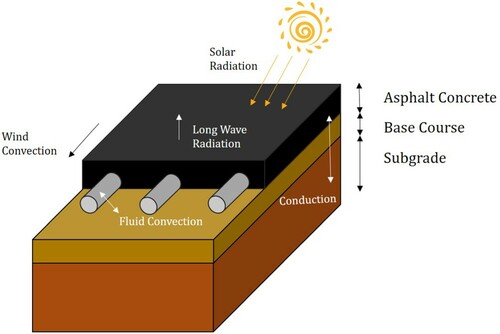
In the asphalt medium, heat is transferred by conduction: (1) ${\rho }_a\cdot c_{p,a}\cdot \frac{\mathrm{\partial }{T}_a}{\mathrm{\partial }t}=\mathrm{\nabla }\cdot \left(-k_a\cdot \overrightarrow{\mathrm{\nabla }}{T}_a\right)$(1) where ${\rho }_a$ is the density of asphalt $(\text{kg}\cdot {\text{m}}^{-3})$; $c_{p,a}$ is the specific heat of asphalt $(\text{J}\cdot \text{k}{\text{g}}^{-1}\cdot {\text{K}}^{-1})$; $k_a$ is the thermal conductivity of asphalt $(\text{W}\cdot {\text{m}}^{-1}\cdot {\text{K}}^{-1})$; and $T_a$ is the asphalt temperature $\left(\text{K}\right)$.

In the fluid medium, heat is transferred by advection–diffusion: (2) ${\rho }_f\cdot c_{p,f}\cdot \left(\frac{\mathrm{\partial }{T}_f}{\mathrm{\partial }t}+\mathrm{\nabla }\cdot \left(\overrightarrow{v}\cdot T_f\right)\right)=\mathrm{\nabla }\cdot \left(-k_f\cdot \overrightarrow{\mathrm{\nabla }}{T}_f\right)$(2) where ${\rho }_f$ is the density of the fluid $(\text{kg}\cdot {\text{m}}^{-3})$; $c_{p,f}$ is the specific heat of the fluid $(\text{J}\cdot \text{k}{\text{g}}^{-1}\cdot {\text{K}}^{-1})$; $k_f$ is the thermal conductivity of the fluid $(\text{W}\cdot {\text{m}}^{-1}\cdot {\text{K}}^{-1})$; and $T_f$ is the fluid temperature $\left(\text{K}\right)$.

As for thermal convection between the circulating fluid and the pipe, the Nusselt number is obtained from the Gneilinski correlation which is specifically catered for circular pipe geometries (Bergman et al., 2011). (3) $N{u}_D=\frac{\left(\frac{f}{8}\right)\cdot \left(R{e}_D-1000\right)\cdot Pr}{1+12.7\cdot \sqrt{\frac{f}{8}}\cdot \left(P{r}^{\frac{2}{3}}-1\right)}$(3) where $f$ is the Darcy friction factor; $R{e}_D$ is Reynolds number; and $Pr$: Prandtl number. All three factors are dimensionless – as is $N{u}_D$. The characteristic length of $N{u}_D$ is defined by the inner pipe diameter, $D_{\mathrm{inner}}$ $\left(m\right)$. The convection coefficient $h_f$ can therefore be obtained as: (4) $h_f=N{u}_D\cdot \frac{k_f}{D_{\mathrm{inner}}}$(4)

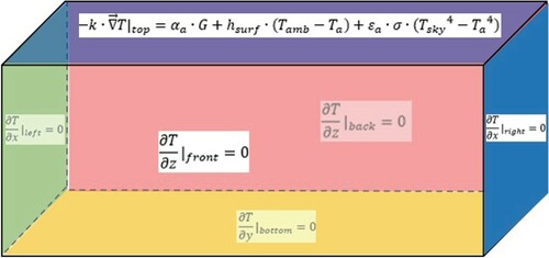
The boundary conditions are shown in Figure 2 where the heat flux is set to zero at all boundaries except the top where the boundary condition is defined to include the combined effects of wind convection, solar radiation, and long-wave radiation governed by the following equation: (5) $-k_a\cdot \overrightarrow{\mathrm{\nabla }}{T}_a{|}_{\mathrm{top}}={\alpha }_a\cdot G+h_{\mathrm{surf}}\cdot \left(T_{\mathrm{amb}}-T_a\right)+{\epsilon }_a\cdot \sigma \cdot \left(T_{\mathrm{sky}}^4-{T_a}^4\right)$(5) where ${\alpha }_a$ is the pavement absorptivity; $G$ is the amount of solar irradiation $\left(\text{W}\cdot {\text{m}}^{-2}\right)$ falling on the pavement; $T_{\mathrm{amb}}$ is the ambient air temperature $\left(\text{K}\right)$; ${\epsilon }_a$ is a ratio that represents the pavement emissivity; $\sigma$ is the Stefan–Boltzmann constant $(5.67\cdot {10}^{-8}\text{W}\cdot {\text{m}}^{-2}\cdot {\text{K}}^{-4})$; and $T_{\mathrm{sky}}$ is the sky temperature $\left(\text{K}\right)$.

Figure 2. Domain boundary conditions.

A direct correlation between the convection coefficient $h_{\mathrm{surf}}$ and the wind speed for a horizontal plate (pavement surface) can be found in the literature (CIBS, 1979): (6) $h_{\mathrm{surf}}=5.8+6.1\cdot v$(6) where $v$ is the wind speed $\left(\text{m}\cdot {\text{s}}^{-1}\right).$

The temperature of the sky is obtained from an empirical correlation (Berdahl & Martin, 1984): (7) $T_{\mathrm{sky}}=\sqrt[4]{{\epsilon }_{\mathrm{sky}}}\cdot T_{\mathrm{amb}}$(7) where ${\epsilon }_{\mathrm{sky}}$ is the ratio that represents the sky emissivity and $T_{\mathrm{amb}}$ is the ambient temperature.

Another empirical correlation is used to obtain the sky emissivity (Berdahl & Martin, 1984): (8) ${\epsilon }_{sky}=\left[0.787+0.764\cdot \log \left(\frac{T_{dp}}{273}\right)\right]\cdot \left[1+0.0224\cdot CC-0.0035\cdot C{C}^2+0.00028\cdot C{C}^3\right]$(8) where $CC$ is the ratio of the cloud cover and $T_{\mathrm{dp}}$ is the dew-point temperature which can be directly related to the ambient temperature by the following simple relation: (9) $T_{\mathrm{dp}}=T_{\mathrm{amb}}-\frac{100-RH}{5}$(9) where $RH$ is the relative humidity $\left(\mathrm{\%}\right)$.

The use of geothermal energy as an energy source for HAP systems follows the same principle of household geothermal heating (Rosen & Koohi-Fayegh, 2017). Various configurations can be devised to allow geothermal energy harvesting, such as: using a horizontal loop of pipes embedded in the ground, a vertical loop of pipes embedded in the ground, and a loop of pipes submerged in a body of water. The heat exchange occurs when the fluid in the pipes extracts (during winter) or rejects (during summer) heat from/into the ground to deliver its intended effect of heating (during winter) or cooling (during summer). These ground-coupled heat exchangers take advantage of the large thermal mass of the soil that dampens temperature fluctuations of the ambient air with increasing depth. Selection between vertical and horizontal loops depends on a number of factors, such as land availability and restrictions on use, soil type and characteristics, costs and limitations on excavation and drilling, among others. Much research has been dedicated towards studying the complex interplay of convection, conduction, and radiation for predicting subsurface temperature distribution. Findings suggest that the influence of the diurnal cycle disappears one metre below the surface, and the effect of seasonal fluctuation is present to a maximum depth of 10 m – with a gradual logarithmic increase for shallower depths (Florides & Kalogirou, 2004; Gehlin & Nordell, 2003; Kurevija & Vulin, 2010).

In this study, a horizontal loop of pipes with an embedment depth of three metres is considered as the ground-coupled heat exchanger configuration used to construct the GCHAP system. The governing equations of the resulting heat transfer processes are similar to those discussed for the modelling of HAPs; whereby, the surrounding media and their properties apply to soil instead of asphalt and air.

4.1.2. Finite difference formulation

The governing partial differential equations of the heat transfer processes are formulated using the Finite Difference Method (FDM) and solved for the prescribed boundary conditions. The discretised equations are programmed in a MATLAB environment. The geometry is automated so that small-scale preliminary simulations can be conducted as well as large-scale simulations.

Since the heat transfer process occurs mainly in the vicinity of the pipe region, a finer mesh is utilised near the pipe; whereas, a coarser mesh is used for the rest of the domain in order to reduce the computational cost. The decision to use a finer mesh in the vicinity of the pipe region also has the added advantage of being able to capture the circular geometry of the pipe using the rectangular elements of finite difference method. The mesh size used in each simulation was decided by a mesh sensitivity analysis carried out for the model geometry and the time step used in the simulations was decided by numerical stability conditions.

The governing equations are discretised explicitly using finite difference equations; whereby, diffusion is discretised using a central-difference scheme, advection using an upwind-difference scheme, and time using forward-difference scheme in accordance with recommendations given in the literature (LeVeque, 2007).

4.1.3. Numerical model calibration and validation

The heat transfer for a plain pavement system can be idealised as a one-dimensional process since all prevalent heat transfer mechanisms occur on the surface of the pavement: solar irradiation, long-wave radiation, wind convection, can be reasonably assumed to occur uniformly. The advantage of a one-dimensional model is that it is computationally less demanding and can therefore be used to run long-term simulations. This is valuable for calibrating the model since the model needs to be run for several days to reach steady state. The resulting predicted steady state temperature distribution is set as the initial condition for a three-dimensional model. The weather data used in the calibration is obtained from the literature (Dakessian et al., 2016). The data is given in 5-minute increments and consists of three parameters: solar flux, ambient temperature, and wind speed. The data is pre-smoothed in order to eliminate the random fluctuations. Figure 3 shows a 7-day simulation.

Figure 3. Temperature variation at: (a) specified depths with time; (b) continuous depths.

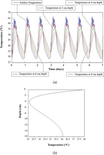
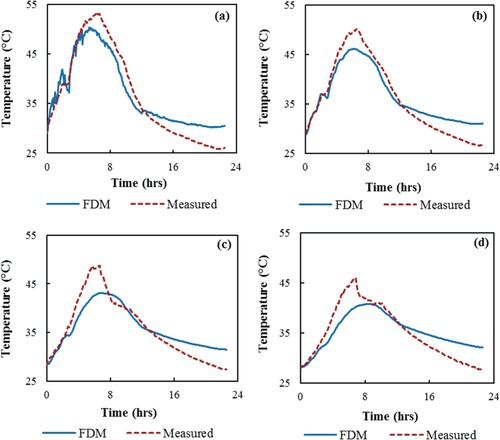
Figure 4 shows a comparison between experimental results obtained from literature (Dakessian et al., 2016) and numerically predicted results obtained from the Finite Difference Model (FDM). The maximum errors of the model are approximately 10%, with an under-prediction of the maximum temperature during daytime, and over-prediction of low temperature at night.

Figure 4. Comparison between measured results and FDM results at: (a) surface; (b) 1.5 cm depth; (c) 4 cm depth; and 6 cm depth.

4.2. Preliminary simulations

4.2.1. Parametric study

After validation, the thermal model is used to simulate the thermal response of the proposed HAP system by controlling the various model parameters: flow rate, pipe spacing, pipe diameter, pipe depth, and thermal conductivity of the pavement. The model geometry and governing parameters are described in Table 2.

Table 2. Reference values of the conducted simulations.

Parameter	Value	Parameter	Value
Weather Conditions
Relative Humidity	65%	Air Temperature	(Dakessian et al., 2016)
Cloud Cover	0.5	Wind Velocity
		Solar Radiation
Reference Model
Pavement Thermal Conductivity	1.3 W/m$\cdot$k	Pipe Diffusivity	24.3 mm^2/s
Pavement Width	4 m	Inlet Temperature	15°C
Pavement Emissivity	0.93	Fluid	Water
Pavement Absorptivity	0.93	Pipe Thickness	2.5 mm
Cross-sectional Depth	16 cm	Pipe Spacing	25 cm
Time of Simulation	12 h	Inner Pipe Diameter	25 mm
Flow Rate	0.2 L/s	Pipe Depth	2.5 cm

A parametric study is performed to assess the impact of varying the different model parameters. The metric used to measure the sensitivity of the parameters is the amount of change of surface temperature (in °C) caused by increasing/decreasing the value of a parameter. Figure 5 shows the results of the parametric study in the form of a spider plot.

Figure 5. Parametric study results.

The parametric study reveals that pavement conductivity and pipe spacing are the most critical to the HAP efficiency since the curves corresponding to the said parameters exhibit the steepest slopes. The depth of the pipes is mildly sensitive, with pipe diameter and flow rate showing the least sensitivity.

4.2.2. Pipe vs. pavement conductivity

Pipe conductivities vary across a very wide range (from 0.3 W/m$\cdot$k for polypropylene (PPR) pipes to 385 W/m$\cdot$k for copper pipes). Figure 6 shows the variation of the surface temperature as a function of the varying pipe conductivity.

Figure 6. Variation of surface temperature with pipe conductivity.

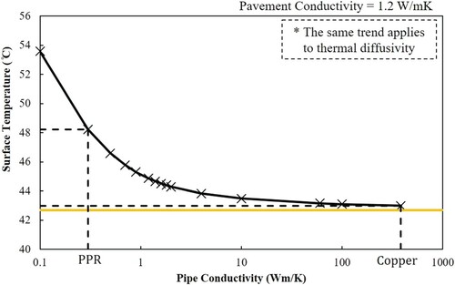
The figure shows that the surface temperature decreases steeply as a function of pipe conductivity – until reaching a certain value where the curve begins to approach an asymptote. This value appears to be the approximate value of the pavement conductivity. Therefore, it can be concluded that the thermal behaviour of HAP is limited by the pavement conductivity. This phenomenon can be best understood by analysing the simplified 1D case: when there are two different materials, the heat flux throughout the combined medium can be given by $q=U\cdot T$ where the overall heat transfer coefficient ($U$) is given as the harmonic mean of $L/K$ of each material $U=1/{\sum }^L/k$. From this, it becomes clear that the heat flux (and thus the rate of heat transfer) is controlled by the bigger $L/K$ ratio. The standard values used in the simulations are: $L1$ = 5 cm, $K1$ = 1.2 W/m$\cdot$K, $L2$ = 0.5 cm. For thermal conductivity of copper ($K2$ = 385 W/m$\cdot$K), U = 24; and for a material whose thermal conductivity is close to asphalt ($K2$ = 1.6 W/m$\cdot$K), U = 22. Clearly, we can see that the difference in $U$ is extremely small given the large relative difference in pipe thermal conductivities. The 3D model agrees with this theoretical analysis since Figure 7 clearly shows that increasing the pipe conductivity beyond that of asphalt has little to no effect. Therefore, instead of investing in expensive pipes, improving the pavement conductivity even by a few percent would yield a better thermal efficiency as can be seen in Figure 7. Such an improvement in pavement conductivity can be achieved by adding graphite to the asphalt mixture (Bai, Park, Vo, Dessouky, & Im, 2015).

Figure 7. Effect of changing asphalt and pipe conductivities on surface temperature.

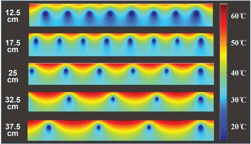
4.2.3. Pipe layout and temperature distribution

To gain deeper insight into the design and performance of a HAP, a critical assessment of the temperature distributions obtained from the simulations is performed. Figure 8 shows the temperature distribution for various pipe spacing. As can be seen in Figure 8, smaller spacing results in not only lower temperatures throughout the pavement but also in a homogenous temperature distribution, which helps in lowering thermal stresses in the pavement. An appropriate design would be one that adequately balances the efficiency and the economic feasibility of the system. Therefore, the choice of spacing needs to consider constructability, economic feasibility, and efficiency. Based on Figure 8, a reasonable choice of spacing would be between 17.5 and 25 cm. Selecting wider spacing would generally result in higher outlet water temperatures.

Figure 8. Effect of spacing on the cross-sectional temperature distribution.

Another important parameter is the pipe depth. Figure 9 (a) shows the temperature distribution for three different pipe depths. The closer the pipe is to the surface, the lower the temperature at the point directly above the pipe. However, the surface temperature between the pipes remains roughly unaffected as the depth increases. As can be observed in Figure 9 (a), the temperature distribution becomes more homogenous as depth increases. From a structural point of view, the increased depth allows for greater stress distribution and thus lower stress experienced by the pipe.

Figure 9. Effect of: (a) depth and (b) diameter on the cross-sectional temperature distribution.

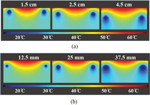
The larger the diameter, the greater the surface area that is in contact with the asphalt pavement. It can be observed from Figure 9 (b) that larger diameters are able to achieve greater reduction in the pavement temperature compared to smaller diameters. However, it is expected that smaller diameters are able to heat the smaller volume of water to a higher degree compared to the larger volume of water passing in large diameter pipes.

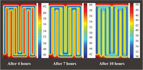
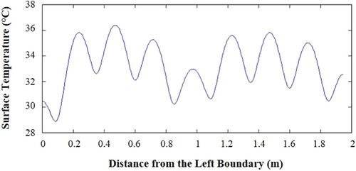
The evolution of surface temperature distribution with time is shown for a reverse-return pipe configuration in Figure 10. One observation is that the surface temperature directly above the pipes is noticeably lower than in other regions within the cross-section. Another important observation is the uniformity of the temperature distribution with time, which reflects the fact that the heat flux from the pipes eventually reaches the surface after a given time.

Figure 10. Evolution of surface temperature distribution with time from numerical simulation.

The crests in Figure 11 represent the temperature between the pipes while the troughs represent the temperature directly above the pipes. Note that the 1st, 4th, 5th, and 8th troughs from the left represent the surface temperature at the pipes for the outgoing fluid. It can be observed that the four aforementioned troughs increase from left to right. This reflects the fact that the fluid is heating up as it circulates from left to right. The inverse can be observed for the four other troughs – 2nd, 3rd, 6th, and 7th since the fluid is circulating in the opposite direction – from right to left.

Figure 11. Surface temperature distribution at the middle of the surface section of the pavement.

4.2.4. Flow rate

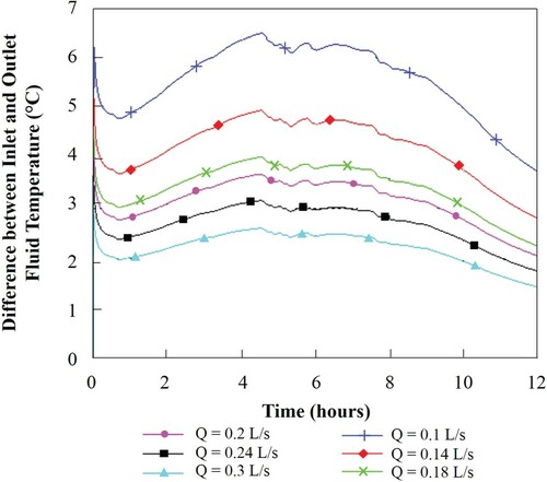
Although the parametric study revealed that changing the flow rate has little effect on the pavement surface temperature; however, the flow rate’s effect on the output fluid temperature was found to be significant.

It can be observed that decreasing the flow rate results in a higher fluid outlet temperature, as illustrated in Figure 12 and consequently a higher surface temperature. This implies that the system becomes less efficient for cooling the pavement when flow rates are low. This can be associated with lower temperature gradient present between the asphalt pavement and the slow circulating fluid. Therefore, the flow rate considered to be used in the built systems is 0.12 L/s.

Figure 12. Effect of flow rate on the temperature difference between inlet and outlet.

4.3. Constructability

The studies done in literature to optimise the HAP system were carried out to increase the efficiency of the system either under controlled lab tests or for a small-scale slab subjected to real weather conditions in the field. The findings of such studies establish the feasibility of the system and list favourable parameters found to be optimum. However, when it comes to paving a road, heavy equipment such as a paver and a vibratory steel drum compactor are involved. Therefore, implementation of a HAP system on large-section warrants studying the placement and support of the pipes, the order and thickness of asphalt lifts to be laid down, the equipment used to compact the lifts, and precautions to be followed to prevent any damage to the pipes during the construction process. In addition, the feasibility of the system is governed by the total cost of implementation, which could be inflated if optimum parameters are used.

The findings in the literature can be summarised as follows: to optimise energy extraction, using a highly conductive material such as copper is encouraged (Carelli, 2010). The depth at which the pipes must be placed must be as close to the surface as possible such that the structural integrity of the system is not compromised (Carelli, 2010; Chen, Rockett, & Mallick, 2008). Smaller pipe diameters must be chosen to yield a higher output water temperature (Deeb, El Jisr, Hotait, Najdi, & Zankoul, 2013; Shaopeng, Mingyu, & Jizhe, 2011). Spacing is dependent on flow rate, but it should be large enough to avoid cool spots, and small enough to increase the efficiency of the system (Mallick et al., 2009). Flow rate must be chosen so as to create a turbulent flow (Shaopeng et al., 2011). The thermal conductivity of the asphalt pavement could be enhanced by using additives such as graphite (Carelli, 2010). Finally, using a serpentine configuration yields higher water temperature than other configurations (Mallick et al., 2009).

In the following, analysis of the findings in the literature will determine whether using the optimum parameters are indeed practical and feasible to construct.

4.3.1. Pipe material

Currently, copper costs 10 USD/m, while polypropylene (PPR) pipes cost 4 USD/m according to a local supplier. Hence, having hundreds of metres of copper pipes in the road would entail high capital cost. Other pipe materials (Table 3) are considered for the study. The main concern in using other materials is its low conductivity compared to that of copper (385 W/m$\cdot$k). However, simulations of the pipe material as illustrated earlier in Figure 5 and Figure 6 prove that the limiting factor to heat transfer is eventually the pavement’s conductivity and not the pipe conductivity. Thus, for the purpose of investigating the possibility of using other pipe material, especially material that can handle the high levels of stress applied by a vibratory steel drum compactor, a pilot study is done on a 4 m² area by changing different parameters. These parameters are presented in Table 3. The condition of the pipes after the small section construction is assessed by pressure-testing. All pipes scenarios demonstrated no leakage except for the 20 mm diameter plastic pipe that was 4 cm below the surface.

Table 3. Pilot study parameters.

Parameter	Value
Piper Diameter (mm)	20
	25
	32
Depth from the Surface (cm)	2
	4
Pipe Placing Technique	Laying on Subgrade
	Laying on Compacted Asphalt Layer
	Spacers
Pipe Material	Steel
	PPR Class 2
	PPR Class 5
	PPR with Aluminium
	Plastic

4.3.2. Thermal conductivity

To improve the thermal conductivity of the asphalt pavement a proposed modification to the asphalt mix is to add graphite powder which has been proven to increase the thermal conductivity of the asphalt mix by up to 2 W/m$\cdot$K (Carelli, 2010). As part of this study, it was found that a 20% replacement of graphite could increase the pavement conductivity by 15%. Graphite, however, was not used later in the project due to limitations on its procurement.

4.3.3. Pipe configuration

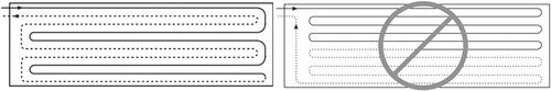
Since the systems are built to be multifunctional in summer and winter, the serpentine configuration recommended in literature couldn’t be used for the pipe network embedded within the asphalt layer for HAP, particularly for the winter application, due to the large surface temperature differential experienced across the area. Instead, a reverse-return layout is considered to provide a uniform temperature distribution across the area as shown in Figure 13 (Uponor Wirsbo, 2003). As for the GCHAP, a serpentine configuration is used for the pipe network embedded at 3 m depth in the soil, which is connected to the reverse-return network with the asphalt layer. The pipe network for the HAP is connected to an external and insulated water tank.

Figure 13. Reverse-return configuration of pipes embedded in the asphalt layer.

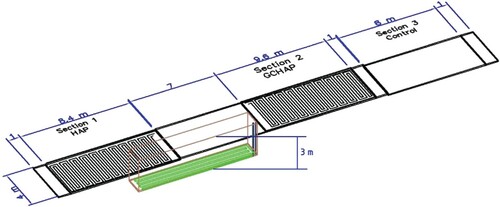
5. Large-scale construction

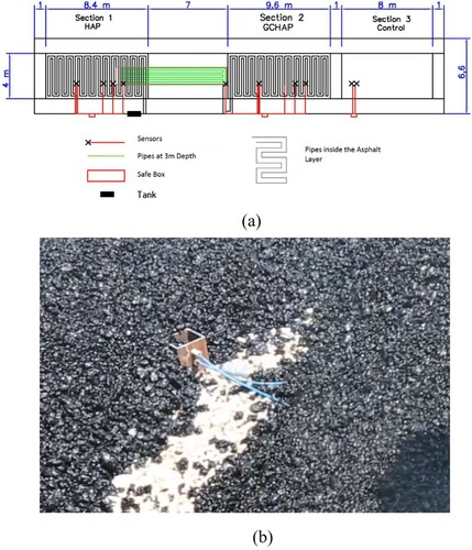
Having performed the numerical simulations to study the effect of each parameter on the temperature distribution of a HAP and after conducting constructability tests to ensure that the chosen parameters are constructible, three large-scale HAP systems are designed: (1) a regular HAP; (2) a ground-coupled HAP (GCHAP); and (3) a control section of no piping network as shown in Figure 14. At a minimum, 1 m-wide buffer zone is allowed between each two sections to preclude any interference of one system on the performance of the other. The positioning of the systems is governed by the location of the GCHAP system and its soil-embedded pipe network. The available locations for the latter network are limited by the presence of installed pipes, conduits, cables, and the waste water system beneath the road.

Figure 14. Schematic of three systems to be constructed.

The process of choosing a location for construction of each system is either facilitated or hindered by various factors including:

• Geometric shape of the road

• Type of soil for GCHAP system

• Shadows cast by nearby objects (trees/buildings/ …) on the considered road

The location for construction is selected to be on a 6 m-wide and 36 m-long piece of a local road in Mesherfeh, Lebanon lying at an altitude of 900 m above sea level. Mesherfeh experiences on average 17 snow days a year, and has an average temperature of 15°C. The road is chosen to be situated in a geological location featuring soil composed of silt and clay to simplify the construction process. The asphalt mix proportions used to pave the three sections are presented in Table 4. The type of stone used in the asphalt mix is limestone, which is widely used in Lebanon. The gradation of mix is shown in Figure 15. Moreover, the road lies along an east–west orientation rather than a north–south orientation to maximise the road’s exposure to sunshine.

Figure 15. Gradation (NMAS 19.0 mm) of the asphalt mixture used in large-scale construction.

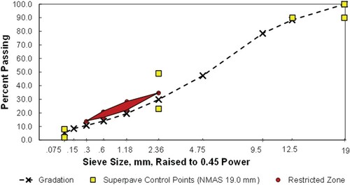
Table 4. Asphalt mix proportioning.

Material	Percentage by Weight of Total Mix
Fine Aggregates (0–6 mm)	39.6%
Intermediate Aggregates (6–12 mm)	30.5%
Coarse Aggregates (12–18 mm)	22.1%
Bag House Fines	3.5%
Binder Content	4.3%

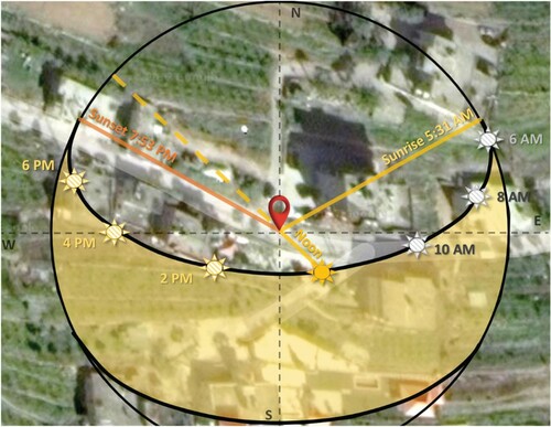
In addition to choosing an east–west orientation for the road, a study for the sun path is conducted to make sure that the selected portion of the road (Figure 16) is not affected by the shadow of the three surrounding properties located at the northeast, southeast, and west directions, as shown in Figure 17.

Figure 16. Road selected for construction of HAP, GCHAP and control sections.

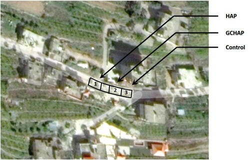
Figure 17. Solar path on 1 July 2017 over the chosen site.

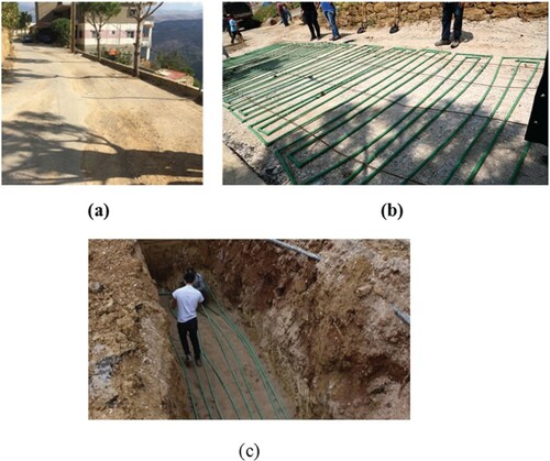
The asphalt layer consisted of a 19.0 mm Superpave mix using PG 64–22 binder and limestone aggregates. Asphalt mix design yielded an optimum asphalt content of 4.3% for 4% air void content. The pipes used are PPR class 2 with outer diameter of 25 mm and inner diameter of 19 mm. The considered spacing is 20 cm. The thickness of the asphalt layer is 6 cm laid on top of a 20 cm thick aggregate base course layer. The pipes are placed directly on top of the base course in a reverse-return layout. Snapshots of the construction process are shown in Figure 18.

Figure 18. Road: (a) before construction; (b) during pipe placement in the asphalt layer; and (c) during pipe placement in the soil (heat sink).

During construction, 46 temperature sensors (thermocouples) were inserted at designated locations and depths within each section to capture the temperature distribution on the surface, across the depth of the pavement, and temperature of circulating water. Figure 19 is a top-view illustration of the locations of these sensors.

Figure 19. (a) Sensors locations on the as-built drawing; and (b) sensor placement in the asphalt layer.

6. Collected field data

Temperature data was collected at the site for a five-day span from 11–16 July, during which the HAP and GCHAP were operating continuously, with water serving as circulating fluid. The measured air temperature and solar flux were typical of those of summer season, with air temperature reaching 32°C.

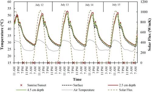
6.1. Control section

The temperature distribution within the control asphalt pavement section is uniform with pavement surface temperatures reaching 50°C as shown in Figure 20. The maximum pavement temperature occurs at a depth of 2.5 cm from the surface. The sharp drop in temperature occurring around 2 pm everyday could be due to a shadow cast by a nearby tree on the location of the measurement sensor. It can be observed that the pavement temperature begins to increase around two hours after sunrise, once heat transfer through radiation and convection are triggered. The solar irradiation is received by the pavement once the sun’s position in the sky allows the sun rays to be directed at the pavement. The air temperature, in turn, gradually starts to increase after sunrise. Accordingly, the temperature of the pavement increases only when radiative heat transfer from the sun’s irradiance takes place alongside the conductive heat transfer from the ambient air.

Figure 20. Temperature distribution for control section.

6.2. HAP section

The temperature distribution within the pavement is clearly influenced by the presence of the HAP components as shown in Figure 21.

Figure 21. Temperature distribution inside the pavement for the HAP section.

The surface temperature for the HAP is not as high as that of the control section as it doesn’t reach 50 °C. Unlike the control section, temperature at 2.5 cm depth from the surface is significantly lower than that of the surface by around 7°C. It’s important to note that the thermocouple at 2.5 cm depth is placed above a pipe carrying fluid that has circulated three quarters of the pipe network, which is henceforth going to be referred to as an outlet pipe as opposed to an inlet pipe that carries fluid that has circulated only a quarter of the length of pipes present in the network. The temperature of the outlet fluid is expected to be higher than that of the inlet fluid; therefore, the effectiveness in decreasing the temperature of the nearby areas is respectively influenced. The temperature fluctuations observed at the surface is also attributed to shade being cast by a nearby tree. Figure 22 shows a full cycle of pavement heating and cooling throughout the day. It can be observed that the temperature at 2.5 cm depth experiences a slower rate of increase compared to that at the surface.

Figure 22. Heating/cooling cycle on 14 July for the HAP section.

It can be observed that there is a lag in temperature increase in the pavement compared to surface temperature, while cooling occurs prior to that at the surface.

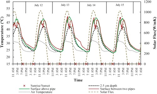
6.3. GCHAP section

The temperature profile for the GCHAP section is shown in Figure 23. Similar to the other sections, fluctuation in surface temperature is observed potentially due to the shade cast by the nearby tree.

Figure 23. Temperature distribution inside pavement (GCHAP section).

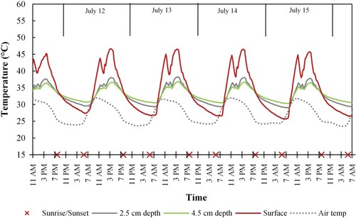
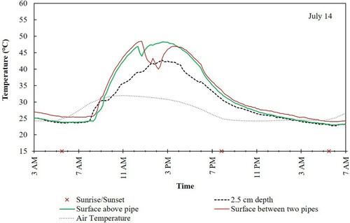
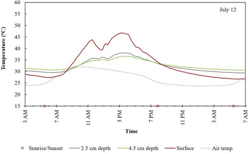
Figure 24 shows a full cycle of pavement heating and cooling throughout the day. The measured temperatures suggest that the GCHAP system has little impact on the surface temperature of the pavement. The temperature recorded at 2.5 and 4.5 cm depth at location situated between two opposing pipes (inlet and outlet) indicates a significant impact of the GCHAP system, where temperatures decrease by around 11°C and 12°C respectively for each depth. The cooling rate of the pavement at a certain depth other than the surface is relatively slow and yields temperatures higher than that of the surface at the end of the cycle. This is attributed to the fact that the circulating fluid is storing the energy harvested from the pavement during the day in the soil and retrieving it at night to influence the pavement temperature.

Figure 24. Heating/cooling cycle on 12 July for the GCHAP section.

In contrast to the HAP, the GCHAP has access to a heat sink (Figure 18(c)) where it can reject the heat collected from the pavement. This yields constant temperature for the fluid entering the asphalt-embedded pipe network as that of the soil after emerging from the pipe network embedded in the ground. In turn, this allows for the continuous presence of a temperature gradient between the pavement and the fluid and consequently a continuous efficient heat transfer.

6.4. HAP vs. GCHAP

Figure 25 shows the effect of each system on the surface temperature of the pavement. It can be observed that both the HAP and GCHAP systems are not effective in reducing the surface temperature. The cooling rate is higher in both HAP and GCHAP systems compared to that of the control. Additionally, the pavement temperature in both GCHAP and HAP systems experiences a lag at the beginning of the cycle compared to the control section. This could be attributed to the circulating fluid that is counteracting the initially small heat transfer occurring.

Figure 25. Comparison of performance of HAP and GCHAP in reducing surface temperature of pavement.

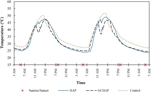
When comparing the temperature at a certain depth of the pavement in each of HAP and GCHAP system, both systems manage to decrease the temperature by a magnitude of approximately 10°C above an inlet pipe, which can be seen individually for each section in Figures 21 and 23. A difference in behaviour is observed in the cooling stage. The temperature of the soil in the GCHAP system yields a higher pavement temperature compared to the control as opposed to a lower pavement temperature showcased by the HAP system.

7. Prediction of pavement performance

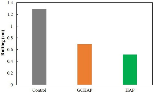
To better understand the gains behind implementing a HAP or a GCHAP system, the decrease in pavement temperature achieved by either systems is translated into an increase in rutting resistance, and thus, longer service life. Rutting prediction is determined through the utilisation of QRSS, Quality-Related Specification Spreadsheet program (Jeong, 2010), relying on the concept of effective temperature (T _eff). T _eff is a single value that represents the temperature at which the resulting distresses are equivalent to distresses caused by the temperature fluctuations that the pavement is subjected to throughout a year (El-Basyouny & Myung, 2009). In this study, T _eff for the control section is calculated using the weather data of the considered site; and whereby, measured temperature reductions for each of HAP and GCHAP sections are applied to the T _eff of the control section to determine the respective effective temperatures for HAP and GCHAP. Other inputs for QRSS include: 6 cm AC thickness, 20 cm subbase thickness, PG64-22 binder content of 4.3% as obtained from a field sample, G _mm of 2.460 as obtained from a field sample, |E*| data as obtained from testing AC samples from the field, and a design speed of 80 km/h. Figure 26 shows the magnitude of rutting reduction associated with using HAP and GCHAP after 20 years.

Figure 26. Rutting prediction associated with each of the three systems.

8. Conclusions

The objective of this study was to construct a HAP on a relatively large-scale section of a road. The incorporation of geothermal energy to operate a HAP was also investigated by constructing another HAP system coupled to a horizontal ground heat exchanger. A thermal numerical model was developed to aid in the design process of the systems. Constructability was studied by conducting lab tests and by carrying out a small-scale pilot study. Finally, a large-scale construction of three systems was executed and documented in a systematic manner. Main conclusions of this study include:

• Having developed a 3D heat transient model, it is now possible to simulate the thermal response of a HAP system consisting of any combination of geometrical and thermo-physical properties.

• The parametric study conducted shows that the surface temperature of the pavement is highly affected by thermal conductivity of the pavement, followed by pipe spacing, depth, diameter, and lastly the flow rate.

• It is more economical to increase the conductivity of asphalt instead of investing money in highly conductive and expensive pipes such as copper.

• It was also established that it is safe to use PPR pipes in HAPs since no damage occurs to them during construction.

• HAP system was found to decrease the surface temperature of the pavement by around 2°C.

• Both GCHAP and HAP were able to decrease the temperature by a magnitude of around 10°C at a 2.5 cm depth with an efficiency that gradually decreases as the fluid circulates the network.

• The temperature stored in the soil in the GCHAP system yields a higher pavement temperature compared to the control opposed to a lower pavement temperature showcased by the HAP system.

• The rutting susceptibility of the pavement decreases for HAP and GCHAP due to the decrease in temperature of the asphalt surface layer.

Based on the findings of this study, future work will consist of collecting pavement temperature data from both HAP and GCHAP during snow time. Moreover, the effect of introducing the pipes on the structural performance of the pavement should be addressed. Other issues that may be caused by the pipes as cracking resistance, adhesion between pipes and asphalt, and moisture damage should be studied.

Acknowledgements

The authors would like to thank Mr. Ahmad El Khatib and Mr. Kamel Saleh for their significant contribution in the development of this work. A special thanks goes to Mr. Helmi Al Khatib and Ms. Dima Al Hassanieh for their tireless efforts. The authors would also like to thank: Dr. Hussein Kassem, Mr. Mazen Shaar, Mr. Abed Al Sheik, Mr. Anis Abdallah, Mr. Khaled Bcharra, Mr. Khaled Joujou, Mr. Fahed Al-Hakim, Mr. Janah Saeed, Dr. Adel Sari Ad Din, the Municipality of Mesherfeh and Advanced Plastic Industries S.A.L (API).

Disclosure statement

No potential conflict of interest was reported by the authors.

References

- Abdel-Khalik, S. I. (1976). Heat removal factor for a flat-plate solar collector with a serpentine tube. Solar Energy , 18 (1), 59–64. doi: https://doi.org/10.1016/0038-092X(76)90036-0
- Asfour, S. , Bernardin, F. , Toussaint, E. , & Piau, J. M. (2016). Hydrothermal modeling of porous pavement for its surface de-freezing. Applied Thermal Engineering , 107 , 493–500. doi: https://doi.org/10.1016/j.applthermaleng.2016.06.138
- Bai, B. C. , Park, D. W. , Vo, H. V. , Dessouky, S. , & Im, J. S. (2015). Thermal properties of asphalt mixtures modified with conductive fillers. Journal of Nanomaterials , 16 (1), 255.
- Barber, E. S. (1957). Calculation of maximum pavement temperatures from weather reports. Highway Research Board Bulletin , 168 , 1–8.
- Berdahl, P. , & Martin, M. (1984). Emissivity of clear Skies. Solar Energy , 32 (5), 663–664. doi: https://doi.org/10.1016/0038-092X(84)90144-0
- Bergman, T. L. , Incropera, F. P. , DeWitt, D. P. , & Lavine, A. S. (2011). Fundamentals of heat and mass transfer . Hoboken, NJ : John Wiley & Sons.
- Bobes-Jesus, V. , Pascual-Muñoz, P. , Castro-Fresno, D. , & Rodriguez-Hernandez, J. (2013). Asphalt solar collectors: A literature review. Applied Energy , 102 , 962–970. doi: https://doi.org/10.1016/j.apenergy.2012.08.050
- Boyd, T. L. (2003). New snow melt projects in klamath falls, OR. Industrial Uses of Geothermal Energy , 12 , 12–15.
- Carder, D. R. , Barker, K. J. , Hewitt, M. G. , Ritter, D. , & Kiff, A. (2008). Performance of an interseasonal heat transfer facility for collection, storage, and re-use of solar heat from the road surface. TRL Published Project Report.
- Carelli, J. J. (2010). Design and analysis of an embedded pipe network in asphalt pavements to reduce the urban heat island effect . Worcester, MA : Worcester Polytechnic Institute.
- Chen, B. L. , Bhowmick, S. , & Mallick, R. B. (2009). A laboratory study on reduction of the heat island effect of asphalt pavements. Journal of the Association of Asphalt Paving Technologists , 78 , 209–248.
- Chen, B. L. , Rockett, L. , & Mallick, R. B. (2008). A laboratory investigation of temperature profiles and thermal properties of asphalt pavements with different subsurface layers. Journal of the Association of Asphalt Paving Technologists , 77 , 327–360.
- Chiou, J. P. (1982). The effect of nonuniform fluid flow distribution on the thermal performance of solar collector. Solar Energy , 29 (6), 487–502. doi: https://doi.org/10.1016/0038-092X(82)90057-3
- Christison, J. T. , & Anderson, K. O. (1972, September). The response of asphalt pavements to low temperature climatic environments. Paper Presented at the Third International Conference on the Structural Design of Asphalt Pavements, Grosvenor House, Park Lane, London, England, Vol. 1.
- CIBS guide book A . (1979). Section A3, CIBS, London.
- Dakessian, L. , Harfoushian, H. , Habib, D. , Chehab, G. R. , Saad, G. , & Srour, I. (2016). Finite element approach to assess the benefits of asphalt solar collectors. Transportation Research Record: Journal of the Transportation Research Board , 2575 , 79–91. doi: https://doi.org/10.3141/2575-09
- Deeb, I. , El Jisr, H. , Hotait, I. A. , Najdi, A. , & Zankoul, E. (2013). Effects of pipe diameter variation in geothermal pavement system. 12th Faculty of Engineering and Architecture Student and Alumni Conference.
- Eggen, G. , & Vangsnes, G. (2005). Heat pump for district cooling and heating at Oslo Airport, Gardermoen. Proceedings 8th IEA Heat Pump Conference, Las Vegas, Nevada, Vol. 30.
- El-Basyouny, M. , & Myung, J. (2009). Effective temperature for analysis of permanent deformation and fatigue distress on asphalt mixtures. Transportation Research Record: Journal of the Transportation Research Board , 2127 , 155–163. doi: https://doi.org/10.3141/2127-18
- Eugster, W. J. (2007). Road and bridge heating using geothermal energy. Overview and examples. Proceedings European Geothermal Congress, Vol. 2007.
- FHWA, US . (2004). Status of the nation’s highways, bridges, and transit: Conditions and performance . Washington, DC : US Department of Transportation.
- Florides, G. , & Kalogirou, S. (2004). Measurements of ground temperature at various depths. Proceedings of the 3rd International Conference on Sustainable Energy Technologies.
- Gehlin, S. E. , & Nordell, B. (2003). Determining undisturbed ground temperature for thermal response test. Transactions-American Society of Heating Refrigerating and Air Conditioning Engineers , 109 (1), 151–156.
- Gui, J. , Phelan, P. E. , Kaloush, K. E. , & Golden, J. S. (2007). Impact of pavement thermophysical properties on surface temperatures. Journal of Materials in Civil Engineering , 19 (8), 683–690. doi: https://doi.org/10.1061/(ASCE)0899-1561(2007)19:8(683)
- Hermansson, Å . (2004). Mathematical model for paved surface summer and winter temperature: Comparison of calculated and measured temperatures. Cold Regions Science and Technology , 40 (1), 1–17. doi: https://doi.org/10.1016/j.coldregions.2004.03.001
- Ho, C. H. , Shan, J. , Du, M. , & Ishaku, D. I. T. (2015). Experimental study of a snow melting system: state-of-practice deicing technology. International Symposium on Systematic Approaches to Environmental Sustainability in Transportation.
- Jeong, M. (2010). Manual of practice HMA quality assurance spreadsheet program using measured values of E* and D . Washington, DC : Transportation Research Board.
- Kassem, H. , Chehab, G. , & Saad, G. (2015). An fem-predictive tool for simulating the cooling characteristics of freshly paved asphalt concrete layers. International Journal of Pavement Engineering , 16 (2), 157–167. doi: https://doi.org/10.1080/10298436.2014.937714
- Kurevija, T. , & Vulin, D. (2010). Determining undisturbed ground temperature as part of shallow geothermal resources assessment. Rudarsko-geološko-naftni Zbornik , 22 (1), 27–36.
- LeVeque, R. J. (2007). Finite difference methods for ordinary and partial differential equations: Steady-state and time-dependent problems . Philadelphia, PA : Society for Industrial and Applied Mathematics.
- Lund, J. W. (1999). Reconstruction of a pavement geothermal deicing system. Geo-Heat Center Quarterly Bulletin , 20 (1), 14–17.
- Mallick, R. B. , Chen, B. L. , & Bhowmick, S. (2009). Harvesting energy from asphalt pavements and reducing the heat island effect. International Journal of Sustainable Engineering , 2 (3), 214–228. doi: https://doi.org/10.1080/19397030903121950
- Minsk, L. D. (1999). Heated bridge technology: report on ISTEA sec. 6005 program (No. FHWA-RD-99-158).
- Pan, P. , Wu, S. , Xiao, Y. , & Liu, G. (2015). A review on hydronic asphalt pavement for energy harvesting and snow melting. Renewable and Sustainable Energy Reviews , 48 , 624–634. doi: https://doi.org/10.1016/j.rser.2015.04.029
- Pletcher, R. H. , Tannehill, J. C. , & Anderson, D. (2012). Computational fluid mechanics and heat transfer . Boca Raton, FL : CRC Press.
- Rosen, M. A. , & Koohi-Fayegh, S. (2017). Geothermal energy: Sustainable heating and cooling using the ground . Chichester : John Wiley & Sons.
- Shaopeng, W. , Mingyu, C. , & Jizhe, Z. (2011). Laboratory investigation into thermal response of asphalt pavements as solar collector by application of small-scale slabs. Applied Thermal Engineering , 31 (10), 1582–1587. doi: https://doi.org/10.1016/j.applthermaleng.2011.01.028
- Siebert, N. , & Zacharakis, E. (2010). Asphalt solar collector and borehole storage: Design study for a small residential building area .
- Solaimanian, M. , & Kennedy, T. W. (1993). Predicting maximum pavement surface temperature using maximum air temperature and hourly solar radiation. Transportation Research Record , 1 , 1–11.
- Sorenson, J. (2006). Resources for a better future. Pavement preservation compendium. Federal Highway Administration, 57-59.
- Thompson, M. R. , Dempsey, B. J. , Hill, H. , & Vogel, J. (1987). Characterizing temperature effects for pavement analysis and design. Transportation Research Record , 1121 , 14–22.
- Timm, D. H. , Voller, V. R. , Lee, E. B. , & Harvey, J. (2001). Calcool: A multi-layer asphalt pavement cooling tool for temperature prediction during construction. International Journal of Pavement Engineering , 2 (3), 169–185. doi: https://doi.org/10.1080/10298430108901725
- Uponor Wirsbo . (2003). Snow and ice melting design manual .
- Van Bijsterveld, W. , Houben, L. , Scarpas, A. , & Molenaar, A. (2001). Using pavement as solar collector: Effect on pavement temperature and structural response. Transportation Research Record: Journal of the Transportation Research Board , 1778 , 140–148. doi: https://doi.org/10.3141/1778-17
- Wang, H. , Wu, S. , Chen, M. , & Zhang, Y. (2010). Numerical simulation on the thermal response of heat-conducting asphalt pavements. Physica Scripta , T139 , 014041. doi: https://doi.org/10.1088/0031-8949/2010/T139/014041
- Yavuzturk, C. , Ksaibati, K. , & Chiasson, A. D. (2005). Assessment of temperature fluctuations in asphalt pavements due to thermal environmental conditions using a two-dimensional, transient finite-difference approach. Journal of Materials in Civil Engineering , 17 (4), 465–475. doi: https://doi.org/10.1061/(ASCE)0899-1561(2005)17:4(465)
- Zwarycz, K. (2002). Snow melting and heating systems based on geothermal heat pumps at Goleniow Airport, Poland .