Predicting the master curves of bituminous mastics with micromechanical modelling

Abstract

The performance of asphalt mixtures is significantly affected by the viscoelastic properties of their mastic phase. The analytical approaches used to predict the properties of mastics from their constituents’ properties are limited in their accuracy and potential to handle non-linear material behaviour. An alternative micromechanical finite element modelling approach to calculate the master curves of mastics from the binder and filler phase properties is presented, where the representative volume elements of mastics consist of linear-viscoelastic bitumen matrices and elastic spherical filler particles. For validation, shear relaxation moduli of bitumen and bitumen-filler mastics are measured at $-10$°C$-80$°C. Additionally, the model is evaluated and compared with the existing analytical solutions. The results indicate that the proposed approach is advantageous as compared to the analytical solutions, as it allows predicting the mastics’ properties over wider temperature, frequency and material ranges at better agreement with the measurements while giving insight into the micromechanical behaviour.

KEYWORDS:

• Bitumen
• asphalt mastic
• multiscale
• master curve
• modelling

Introduction

The viscoelastic properties of the bituminous mastic significantly influence the overall mixture performance. In particular, the composition of mastics and their mechanical properties have been shown to affect fatigue as well as rutting resistance of asphalt mixtures (Faheem et al., 2008). Several analytical and numerical modelling approaches to predict the mastic properties from its constituents’ volumetric and mechanical characteristics exist in the literature (Buttlar et al., 2007; Faheem & Bahia, 2012; Ma, Chen, Yang, et al., 2019). However, as reported in several studies, there are certain limitations to the aforementioned models; specifically, their limited accuracy at higher temperatures (Ma, Chen, Yang, et al., 2019) and high volume fractions (Buttlar et al., 2007). In order to improve mastic modelling accuracy and applicability, several studies proposed numerical micromechanical models of mastic based on the finite element and discrete element methods, cf. e.g. Hesami et al. (2014), Tehrani et al. (2018) and Abbas et al. (2005), respectively. A recent study by Fadil et al. (2020) presented a new micromechanical FE model for the prediction of mastic’s viscoelastic properties. The proposed model allows for predicting the complex moduli, $G^{\ast }(\omega ),$ and phase angles, $\delta (\omega ),$ of mastics from their volumetric composition and binder properties in a computationally efficient manner. In the model, the filler phase is represented as elastic particles randomly distributed in a viscoelastic binder matrix. A representative volume element (RVE) of mastic is generated and used to calculate homogenised viscoelastic properties of mastic from its response to a uniaxial tensile load. In order to validate the developed model, $G^{\ast }(\omega )$ and $\delta (\omega )$ of several mastics were measured with the Dynamic Shear Rheometer (DSR) at a temperature range of $0-{10}^{\text{o}}$C. For the limited range of temperatures examined in Fadil et al. (2020), it was shown that the developed model allows for predicting the viscoelastic properties of mastics accurately for the studied materials.

This paper aims to investigate the applicability of the modelling approach proposed by (Fadil et al., 2020) for predicting the viscoelastic properties of mastics in a broader temperature range as well as to evaluate the effect of the composition of a mastic material on its linear-viscoelastic limit. Shear relaxation moduli of bitumen and bitumen-filler mastics are measured with DSR at temperatures from $-10$°C to $80$°C and master curves are constructed for each material. The FE models of mastics are set-up following the procedure proposed in (Fadil et al., 2020), incorporating measured shear relaxation modulus of bitumen as well as the measured size distribution of the filler. The capability of the models to capture the measured response of mastic materials is evaluated and discussed. The shear relaxation moduli of mastics are also calculated with the generalised self-consistent scheme (GSCS) approach (Christensen & Lo, 1979) and the results are compared with the ones obtained from the proposed model. Furthermore, the use of micromechanical FE modelling allows for potentially gaining better insight into the non-linear behaviour of mastic materials. In order to, at least partially, evaluate the feasibility of the proposed modelling approach with respect to capturing non-linear material behaviour, it is presently applied to examine the relationship between the filler volume fraction and the mastic’s linear-viscoelastic (LVE) limit. Accurate identification of the LVE limit is a crucial first step for predicting mastic’s non-linear behaviour, as it represents a starting point for accumulation of viscoplastic deformation or damage in the material. The modelling predictions are compared to the Dynamic Shear Rheometer (DSR) measurements and to the results reported in the literature (Chaudhary et al., 2020; Ma, Chen, Gui, et al., 2019).

Methodology

In this study, a micromechanical modelling approach, suitable for capturing viscoelastic properties of mastic over a wide temperature range is established following the developments in Fadil et al. (2020). The established model is used to examine the viscoelastic behaviour of mastic in the temperature range from $-10$°C to $80$°C and at two volumetric filler concentrations, $\varphi =$ 30% and 50%. Both studied mastics are prepared by mixing penetration grade 70/100 bitumen with quartz sand filler. In order to provide the input parameters for the model, the bitumen’s viscoelastic properties and filler size distribution have been measured, as detailed in the Experimental study section. To validate the model, the calculated effective viscoelastic properties of mastic are compared with those measured with the DSR. Modelling and experimental methodology used in this study is described in detail below.

Computational modelling

A bitumen-filler mastic is a composite material consisting of a viscoelastic binder and elastic filler particles. Therefore, the micromechanical modelling procedure employed presently uses a two-phase model. The model utilises a cubic RVE as shown in Figure 1, along with the coordinate system and loading used in this study. The filler is idealised as spherical inclusions randomly distributed within a viscoelastic matrix, representing the binder phase. The spherical inclusions are distributed randomly within the RVE using the open-source molecular dynamics software Large-scale Atomic/Molecular Massively Parallel Simulator (LAMMPS). The use of LAMMPS allows for obtaining an RVE with a high concentration of spherical inclusions (up to a volume fraction, $\varphi$, of 65% for the particles size distribution used in this study). This is achieved by using a three-step simulation process in LAMMPS. First, the spheres are dropped randomly under gravity into a box with x, y and z dimensions of $L\times L\times 2L$, where $L$ is the length of the RVE cube. The spheres are originally generated with a diameter that is 5% larger than the target value. In the second step, the wall in the z-direction is lowered to compact the spheres within the RVE volume. In the final step, the bottom wall is vibrated to resettle the particles and lower the stresses developed within the spheres due to compaction. The spherical inclusions coordinates and diameters are then transferred to ABAQUS where the RVE is constructed and the finite element analysis is performed. At this step, in order to ensure that there is no contact between the filler particles in the model, the diameters of spheres are reduced by 5%. The matrix is then created around the inclusions with a wall dimension of $L$. The model was meshed with the tetrahedral quadratic elements with hybrid formulation in ABAQUS, variable size controls were employed resulting in approximately 500e3 elements generated for every model.

Figure 1. The representative volume element used for the model with $\varphi =$ 30%, loaded uniaxially.

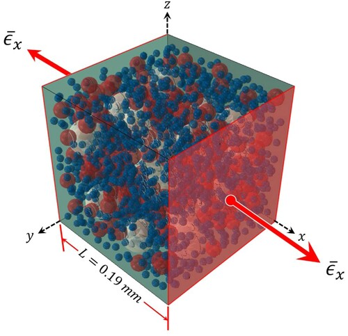
As shown in Figure 1, the loading of the RVE is performed uniaxially in strain control by applying an effective strain instantaneously: (1) ${\overline{ϵ}}_x(t)={ϵ}_o\cdot H(t=0)$(1) where ${\overline{ϵ}}_x$ is the volume average strain in the x-direction, ${ϵ}_o$ is the strain magnitude, and $H(t)$ is the Heaviside step function.

Periodic boundary conditions (PBC) are utilised in order to simulate an infinite volume with a periodically repeating microstructure, defined by the RVE. This is achieved by tying the displacement degrees of freedom of nodes on the opposing faces using equations in ABAQUS. The use of PBC allows for reducing the model size considerably while maintaining the accuracy (Gitman et al., 2007), thus, improving upon the computational efficiency.

Volume average stress, ${\overline{\sigma }}_x(t)$, and strains, ${\overline{ϵ}}_x(t)$, ${\overline{ϵ}}_y(t)$, ${\overline{ϵ}}_z(t)$, are obtained from the model and used to calculate the homogenised properties of mastic in the time domain, i.e. viscoelastic Poisson’s ratio $\overline{\nu }(t)$ and relaxation function $\overline{E}(t)$ as in Equations (2) and (3): (2) $\begin{array}{rl}\overline{\nu }(t)& =-\frac{{\overline{ϵ}}_y(t)+{\overline{ϵ}}_z(t)}{2{\overline{ϵ}}_x(t)}\end{array}$(2) (3) $\begin{array}{rl}\overline{E}(t)& =\frac{{\overline{\sigma }}_x(t)}{{\overline{ϵ}}_x(t)}\end{array}$(3)

Afterwards, $\overline{E}(t)$ is used to calculate the shear relaxation function $\overline{G}(t)$ using the linear elastic relationship between the material constants combined with the viscoelastic correspondence principle as in Equations (4) and (5): (4) $\begin{array}{rl}G& =\frac{E}{2(1+\nu )}\end{array}$(4) (5) $\begin{array}{rl}s\times \tilde{G}(s)& =\frac{s\times \tilde{E}(s)}{2(1+s\times \tilde{\nu }(s))}\end{array}$(5) where $\tilde{G}(s)$, $\tilde{E}(s)$ and $\tilde{\nu }(s)$ are the Laplace transforms of $\overline{G}(t)$, $\overline{E}(t)$ and $\overline{\nu }(t)$ respectively. Using the Park and Schapery exact method (Park & Schapery, 1999), $\overline{G}(t)$ and $\overline{\nu }(t)$ are transformed then to their frequency domain counterparts, i.e. complex modulus and Poisson’s ratio $G^{\ast }(\omega )$ and ${\nu }^{\ast }(\omega )$.

The modelling approach described above explicitly captures the influences on the rheology of mastic from the filler volume fraction, its linear elastic properties and size distribution, and from the viscoelastic properties of the binder. However, there are other parameters that have been reported to affect the viscoelastic properties of mastics. In particular, filler shape, texture and possible bitumen-filler chemical interactions are known to influence the rheology of the mastics (Buttlar et al., 2007). In order to account for those parameters, at least indirectly, Fadil et al. (2020) proposed a calibration procedure, which was concluded in their study that it improves the degree of agreement between model and experiments within the temperature range $0-10$°C. The procedure consists of adjusting the volumetric filler concentration, i.e. creating models with effective filler concentrations, ${\varphi }_e$, in order to account for the stiffening mechanisms that are not explicitly modelled. The approach is adopted in this study for the expanded temperature range, where ${\varphi }_e$ is given by: (6) ${\varphi }_e=C_v\times \varphi$(6) with $C_v$ as calibration factor, determined with the following procedure. 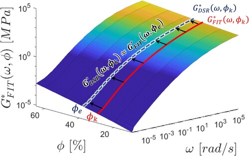In order to calculate $C_v$, the response of the model due to the frequency and the volume fraction needs to be quantified. For achieving that, the model results, in terms of effective complex modulus of mastics,$G_{FEM}^{\ast }({\omega }_k,\varphi ),$ over the filler concentrations in the range of $\varphi =$ 10–65%, are fitted with Equation (7): (7) $G_{FIT}^{\ast }({\omega }_k,\varphi )=a_k\cdot e^{b_k\times \varphi }+c_k\cdot e^{d_k\times \varphi }$(7) where $G_{FIT}^{\ast }$ is the fitted $G_{FEM}^{\ast }$ for specific frequency value $\omega ={\omega }_k$ and the variables $a_k$, $b_k$, $c_k$ and $d_k$ are parameters used for fitting the function using nonlinear regression by minimising Equation (8): (8) $Min\left|{\left(\frac{G_{FIT}^{\ast }({\omega }_k,\varphi )-G_{FEM}^{\ast }({\omega }_k,\varphi )}{G_{FEM}^{\ast }({\omega }_k,\varphi )}\right)}^2\right|$(8)

A two-term exponential function in Equation (7) is chosen as it was found to provide a good fit with $R^2>$ 0.99 for all values of ${\omega }_k$. The obtained response surface is shown in Figure 2. For a given $\varphi ={\varphi }_k$ the corresponding ${\varphi }_e$ is found by locating the complex modulus measured with the DSR for mastic with filler concentration ${\varphi }_k$, $G_{DSR}^{\ast }(\omega ,{\varphi }_k)$, on the response surface as illustrated in Figure 2. This can be done through minimising the difference between $G_{DSR}^{\ast }(\omega ,{\varphi }_k)$and $G_{FIT}^{\ast }(\omega ,{\varphi }_e)$, as shown in Figure 2, according to Equation (9): (9) $Min\sum _{{\varphi }_k={\varphi }_{min}}^{{\varphi }_{max}}\left|\sum _{{\omega }_k={\omega }_{min}}^{{\omega }_{max}}{\left(\frac{G_{FIT}^{\ast }({\omega }_k,{\varphi }_e)-G_{DSR}^{\ast }({\omega }_k,{\varphi }_k)}{G_{DSR}^{\ast }({\omega }_k,{\varphi }_k)}\right)}^2\right|$(9) Afterwards, the calibration factor $C_v$ can be calculated from Equation (6).

Figure 2. The response surface for the calculated complex modulus as a function of radial frequency and volume fraction.

There are several analytical models in the literature capturing the stiffening effect of the filler on mastic. In particular, GSCS has been extensively used on bitumen-based mastics (Buttlar et al., 2007; Ma, Chen, Yang, et al., 2019; Yin et al., 2008). While GSCS may not explicitly capture the effects of the filler size distribution and the filler particles interaction on mastics rheology, it has an important advantage of being relatively simple as compared to the numerical approaches. Thus, it seems to be of interest to compare the proposed micromechanical modelling with the GSCS findings. In GSCS the equations are described by Christensen and Lo (1979) and they follow the format of Equation (10)(10) $A{\left(\frac{G_{mastic}}{G_m}\right)}^2+B\left(\frac{G_{mastic}}{G_m}\right)+C=0$(10) : (10) $A{\left(\frac{G_{mastic}}{G_m}\right)}^2+B\left(\frac{G_{mastic}}{G_m}\right)+C=0$(10) where $G_{mastic}$ is the calculated complex shear modulus of the mastic, and $G_m$ is the complex shear modulus of the bitumen matrix. $A$, $B$ and $C$ are variables that depend on the stiffness ratio $G_m/G_i$ as well as ${\nu }_m$ and ${\nu }_i$, where $G_i$ is the complex shear modulus of the inclusions, and ${\nu }_m$ and ${\nu }_i$ are the Poisson’s ratios for the matrix and inclusions respectively. To find $G_{mastic}$ Equation (10)(10) $A{\left(\frac{G_{mastic}}{G_m}\right)}^2+B\left(\frac{G_{mastic}}{G_m}\right)+C=0$(10) is solved as a quadratic equation giving: (11) $G_{mastic}=\frac{\sqrt{B^2-4AC}-B}{2A}{G}_m$(11)

As demonstrated by Yin et al. (2008) the problem can be simplified by assuming rigid inclusions ($G_i\to \mathrm{\infty }$) and a nearly incompressible matrix (${\nu }_m\to 0.5$). In this simplified form $G_{mastic}$ only depends on $\varphi$, therefore, it has a constant value regardless of the stiffness ratio between the filler and mastic. In turn, these assumptions make the formula independent of temperature and measurement frequency.

Experimental study

For the DSR measurements, bitumen-filler mastics specimens were prepared by mixing the base bitumen, with penetration grade of 70/100, with quartz sand filler. Mastics were prepared with two volumetric filler concentration, $\varphi =$ 30% and 50%. The amounts of fillers corresponding to the target $\varphi$ were determined based on its density, measured with the pycnometer method to be 2.69 ± 0.02 g/cm³. Complex moduli, $G^{\ast }(\omega )$, for base bitumen and for the mastics with $\varphi =$ 30% and 50% (marked ‘Bitumen’, ‘BQ30’ and ‘BQ50’ through the rest of the paper), were measured with DSR (two replicates per material) according to AASHTO T 315. Tests were performed for the temperature range from $-{10}^{\text{o}}$C to ${80}^{\text{o}}$C with ${10}^{\text{o}}$C increments, and at the angular frequencies $\omega =$ 0.22–62.83 rad/s. The variability between the repetitions for the same material was found to be within 10% for most of the measurements and never exceeding 20%. Based on the measurements, the master curves have been constructed for the $G^{\ast }(\omega )$ of each material as presented in Figure 3.

Figure 3. Master curves built for bitumen and mastics showing the complex modulus and the phase angle at a reference temperature $T_{ref}={20}^{\circ }\text{C}$.

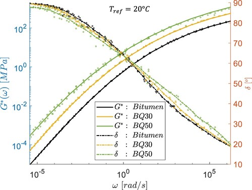
The results were shifted to the reference temperature $T_{ref}=$ 20°C. The master curves in Figure 3 were constructed using the shift factors ($a_T$) obtained from the Williams–Landel–Ferry equation: (12) $\log (a_T)=-\frac{C_1(T-T_{ref})}{C_2+(T-T_{ref})}$(12) where $T$ is the temperature of measurement and $C_1$ and $C_2$ are the constants of the WLF equation shown in Table 1. The measured bitumen’s complex modulus is used to define $G^{\ast }(\omega )$ of the binder phase in the model as well as in GSCS calculations.

Table 1. Williams–Landel–Ferry constants.

Material	$C_1$	$C_2$
Bitumen	19.82	160.28
BQ30	19.54	150.12
BQ50	20.43	146.02

As can be seen in Figure 3, the addition of filler makes the mastic stiffer, with $G^{\ast }(\omega )$ about 2.5–5.6 times the bitumen value for bitumen and $G^{\ast }(\omega )$ for BQ50 about 5–30 times that of bitumen. On the other hand, the phase angles do not change much with the addition of filler, with the largest change occurring for BQ50, where the phase angle does not reach 90${}^{\circ }$ even at the lowest frequencies tested. This may be due to the higher effect of particles interactions at high filler concentration (Buttlar et al., 2007; Faheem & Bahia, 2012).

The linear-viscoelastic (LVE) limit was determined for bitumen and BQ30, from strain sweep tests performed at 5°C using the DSR at $\omega =$ 10 rad/s. The criterion used to define the LVE limit is the decrease of $G^{\ast }(\gamma )$ to 95% of its initial value (Petersen et al., 1994). Therefore, it was determined that the shear strain limit is approximately ${\gamma }_{LVE}=$ 1% and ${\gamma }_{LVE}=$ 0.34% for bitumen and BQ30 respectively.

Volumetric behaviour of the binder phase is defined through the complex Poisson’s ratio ${\nu }^{\ast }(\omega )$, calculated from assumed constant bulk modulus for the binder, i.e. $K^{\ast }(\omega )=K_o$. The $K_o$ value is taken as 2.34 GPa based on the measurements reported by Wolf (2010). The frequency-domain functions,$G^{\ast }(\omega )$ and ${\nu }^{\ast }(\omega )$, are transformed to the time domain using the Park and Schapery exact method (Park & Schapery, 1999).

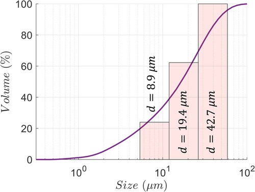
Regarding the filler phase in the model, the elastic properties were taken to be, $E=70$ GPa, $\nu =$ 0.17, according to data in (Quartz Crystal (SiO2), 2012). The size distribution of the quartz sand filler has been measured using a laser diffractometer instrument. The measured size distribution as well as the corresponding simplified distribution, used in the model, are shown in Figure 4. Particles with sizes within the range 5.92–51.80 µm quartz filler were considered for the model in order to reduce the computational time. Particles outside this range were added proportional to the volume fraction to the sizes chosen, denoted $d$ in Figure 4.

Figure 4. The size distribution of the quartz filler as well as the simplified size distributions used in the model, $d$ denotes the particle diameter.

Results and discussion

From the DSR measurements the master curves are constructed for bitumen, BQ30 and BQ50 materials. These master-curves are shown in Figure 5(a,b) for BQ30 and BQ50 materials, the bitumen master curve is included in both figures for comparison. Similar to the results reported previously (Buttlar et al., 2007; Fadil et al., 2020; Faheem & Bahia, 2012), the addition of filler stiffens the mastics. However, as it may also be seen from the DSR results in Figure 5, this stiffening effect is also frequency dependent, as the deviation between bitumen and mastics curves increases with decreasing $\omega$. Also shown in Figure 5, master curves predicted for BQ30 and BQ50 with the model described in the previous section are presented. The modelling results in Figure 5 are shown as obtained at $\varphi$  30% and 50% for BQ30 and BQ50 materials as well as calculated at their corresponding ${\varphi }_e$ cf. Equation (6)(6) ${\varphi }_e=C_v\times \varphi$(6) . Using Equation (6)(6) ${\varphi }_e=C_v\times \varphi$(6) it was calculated that $C_v=1.218$, with the described calibration procedure. As shown in Figure 5(a,b), the modelling results tend to somewhat underestimate the $G^{\ast }(\omega )$ of mastics with deviations between the measurements and modelling results increasing with increasing $\varphi$ and decreasing $\omega$. At the same time, results in Figure 5 demonstrate that the calibration improves the modelling accuracy significantly. The $G^{\ast }(\omega )$ predicted with the calibrated model does not deviate more than 30% from the experimental values, except for the case of BQ50, at $\omega <{10}^{-1}$ rad/s. Thus, it may be concluded that the modelling approach presented, captures the viscoelastic response of mastics reasonably well for the full temperature range considered.

Figure 5. The calibrated model $G^{\ast }(\omega )$ compared to model before calibration and the experimental values for (a) ϕ = 30%, (b) ϕ = 50%, at reference temperature $T_{ref}={20}^{\circ }\text{C}$.

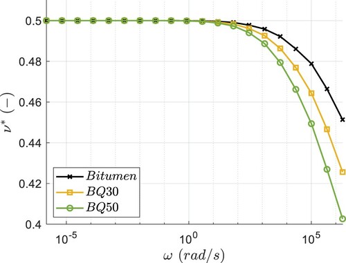
Figure 6 shows the bitumen’s ${\nu }^{\ast }(\omega )$ calculated from the measured $G^{\ast }(\omega )$ and the assumed $K_o$, along with ${\nu }^{\ast }(\omega )$ obtained from the models for BQ30 and BQ50. The figure shows that the assumption of constant bulk modulus results in a ${\nu }^{\ast }(\omega )$ that asymptotically increases to 0.5 as the frequency decreases, which is in line with the experimental observations by Benedetto et al. (2007). The computationally predicted ${\nu }^{\ast }(\omega )$ of mastic, shown in Figure 6, exhibit frequency dependency similar to the one of bitumen. As seen in Figure 6 however, the addition of filler decreases ${\nu }^{\ast }$ of mastic at high frequencies.

Figure 6. ${\nu }^{\ast }(\omega )$ for the bitumen and calculated ${\nu }^{\ast }(\omega )$ for the mastics obtained from FE simulations at a reference temperature $T_{ref}={20}^{\circ }\text{C}$.

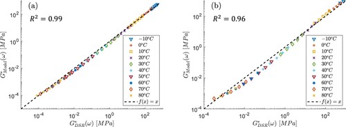
In order to evaluate the agreement between the model and DSR measurements quantitatively, in Figure 7 the complex modulus obtained with the DSR, $G_{DSR}^{\ast }(\omega )$, is compared to the one obtained with the calibrated model, $G_{Model}^{\ast }(\omega )$. The dotted line in Figure 7 represents the equality line. For BQ30, with a relatively low filler volume fraction, a very good agreement between the experimental and modelling results is observed with $R^2=$ 0.99. On the other hand, the DSR and modelling results largely agree for BQ50, with $R^2=$ 0.96, considerable deviations do, however, appear at higher temperatures (i.e. $T\ge {40}^{\circ }$C) where the stiffness of the matrix becomes very low in contrast to the inclusions. This can be attributed to the idealisation of the structure using spherical inclusions instead of the actual shapes of the filler particles; as silica-based particles are known to be angular (Hesami et al., 2014).

Figure 7. Equality plots for the measured DSR results as compared to the calibrated modelling results for (a) BQ30 and (b) BQ50.

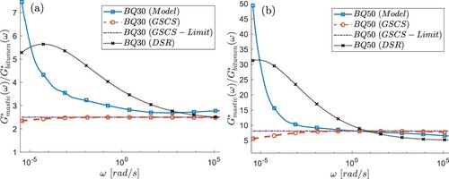
Numerical and experimental stiffness ratios,$G_{mastic}^{\ast }(\omega )/G_{bitumen}^{\ast }(\omega )$, are presented in Figure 8, along with the ones, obtained based on two analytical solutions: generalised self-consistent scheme (GSCS) developed by Christensen and Lo (1979) and the simplified limit value calculation (Yin et al., 2008). The Full GSCS solution does not fully capture the frequency sensitivity of the stiffness ratios found in the experimental results. This difference seems to occur at low frequencies where the stiffness contrast is highest due to its inability to capture the particles interaction stiffening effect (Buttlar et al., 2007). At the same time, the simplified limit value calculation, results in stiffness ratios which are completely frequency independent. By contrast, the stiffness ratios predicted numerically generally increase with decreasing $\omega$, as also observed from the DSR measurements. As seen in Figure 8, this occurs due to the increase in stiffness contrast between the filler and binder phases, where the effect of the microstructure becomes more prominent especially at high volume fractions (Gusev, 2016).

Figure 8. Comparison of the stiffness ratio obtained using the developed model, the generalised self-consistent scheme (GSCS), and the GSCS with limit values for (a) ϕ = 30%, (b) ϕ = 50%, at a reference temperature$T_{ref}={20}^{\circ }\text{C}$.

In addition to capturing macro-mechanical properties of mastic, the presented micromechanical model is capable of gaining further insight into the local concentrations of stresses and strains for further analysis, with respect to e.g. fatigue or viscoplasticity analysis. Figure 9 shows the distribution of the shear strain in a slice located at $z=L/2$. These distributions are obtained by loading the RVE in pure shear with effective shear strain of $\overline{\gamma }=$ 0.2% and 0.34% for the models with $\varphi =$ 10%, 30% and 50% with at a frequency of $\omega =10rad/s$. As the figure shows, the existence of the filler particles introduces strain concentrations within the RVE. For example, the local strains are within 1–2 times the applied strain for $\varphi =$ 10%, however, at $\varphi =$ 50%, the maximum shear strain can increase to approximately 10 times the one applied on the macro level. Increasing the value of $\overline{\gamma }$ from 0.2% to 0.34% increases the local concentrated strain within the matrix more than it does for the filler particles. As can also be surmised from the figure at a high volume fraction, i.e. $\varphi =$ 50%, there is the tendency for the load to be transferred through the particles interaction as evidenced by the concentrations of shear strains between close filler particles. This is in agreement with the literature (Buttlar et al., 2007; Faheem & Bahia, 2012; Hesami et al., 2012), as it is reported that at higher filler concentrations the particles interaction effects become more prominent.

Figure 9. The maximum shear strain distribution within the micromechanical model at $z=L/2$ for applied effective shear strains 0.2% and 0.34% and for three filler volume fractions, $\varphi =$ 10%, 30% and 50% at reference temperature $T_{ref}=5^{\circ }\text{C}$ and $\omega =10\text{ rad/s}$.

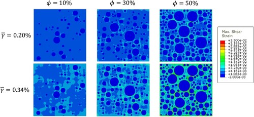
Figure 10. (a) Volume exceeding the linear-viscoelastic limit for two applied shear strains and (b) the corresponding element representation of said volume at reference temperature $T_{ref}=5^{\circ }\text{C}$.

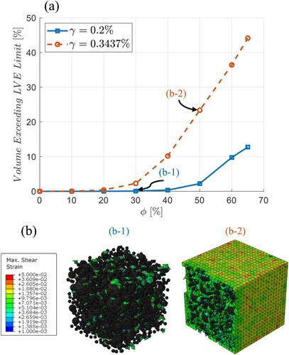
In what follows, the effect of strain localisations around filler particles, illustrated in Figure 9, on the linearity limit of the mastics is examined. In the analysis, the LVE limit for the binder phase is assumed to be equal to the ${\gamma }_{LVE}$ measured for the pure bitumen with DSR at $5^{\circ }C$ of measurement temperature, i.e. ${\gamma }_{LVE}=$ 1%. The proportion of the binder phase experiencing strains higher than ${\gamma }_{LVE}$ is examined for the cases of RVEs of mastic under the action of two shear strain levels $\overline{\gamma }=$ 0.2% and 0.34% and for materials with filler concentrations, $\varphi =$ 10–65%. The results of this analysis are depicted in Figures 10, where Figure 10(a) shows the binder phase volume subjected to strains above the LVE limit as a function of $\varphi$. The visualisation of the binder phase volume subjected locally to the strains exceeding the LVE limit is presented in Figure 10(b) for the mastics with $\varphi =$ 30% and 50% subjected to $\overline{\gamma }=$ 0.2% and $\overline{\gamma }=$ 0.34% respectively. As seen in Figure 10(a), the volume of the binder that exceeds the LVE limit is dependent on both $\overline{\gamma }$ and $\varphi$; increasing the volume fraction of filler increases the volume of the binder that exceeds the LVE limit at the same value of $\overline{\gamma }$. Thus, it may be expected that the presence of filler may result in lower LVE limit for the mastic as compared to the one of the base binder, due to strain localisation in the binder phase. This finding is in line with the observations from the DSR strain sweep tests where ${\gamma }_{LVE}$ for BQ30 has been measured to be approximately 30% of the binder’s ${\gamma }_{LVE}$. Similar observations, i.e. a decrease in the LVE limit with increasing filler volume fraction, have been reported by (Ma, Chen, Gui, et al., 2019) based on the DSR measurements performed on neat binders and SBS modified binders and varying limestone filler contents ($\varphi =$ 23–68%). Additionally, the results in Figure 10(a) confirm that $\overline{\gamma }=$ 0.2% used with the DSR tests is within the LVE range for the tested mastics BQ30 and BQ50 the volume that exceeds the LVE range is less than 2.2% which is expected not to influence the results significantly.

In summary, the micromechanical modelling approach proposed by Fadil et al. (2020) appears to be advantageous as compared to analytical solutions as it allows one to better capture the viscoelastic properties of the mastic and account for the frequency dependence of the stiffness ratios over wide temperature range, as illustrated with Figure 5, Figure 7 and Figure 8. Furthermore, the micromechanical modelling allows for gaining a better understanding of the local phenomena governing the mastic’s macro-scale response as illustrated with the results presented in Figures 9 and 10.

Conclusions

The viscoelastic behaviour of bitumen-filler mastics has been examined experimentally and numerically. The main findings of the study are summarised as follows:

1. The proposed micromechanical modelling approach accurately captures the measured shear relaxation moduli of mastics for a wide temperature range, i.e. from $-10$°C to $80$°C. The agreement between the calculated and measured shear relaxation moduli was generally found to be within 30%, when the simulations were performed at effective filler concentrations, adjusted through the described calibration procedure.

2. Based on the comparison of the stiffness ratios obtained with the proposed micromechanical finite element (FE) model and the generalised self-consistent scheme (GSCS), it is shown that the modelling approach is advantageous both in terms of accuracy and calculation robustness as compared to the GSCS. The GSCS was calculated in its full form as well as a simplified form that assumes rigid inclusions and incompressible matrix. However, it appears that the differences between the modelling approach and experimental results increases at higher filler concentrations and temperatures, i.e. T $\ge {40}^{\circ }$C. This can be due to the increased effect of particle-to-particle interactions, which is not fully captured due to the spherical particle shape assumed in this work.

3. Viscoelastic Poisson’s ratios of the mastics that are obtained numerically decrease with increasing filler concentrations and demonstrate reasonable trends with respect to frequency dependence.

4. The use of FE analysis opens the opportunity for gaining insight into the local micromechanical behaviour. In particular, the developed model has been used to examine the effect of filler content on mastics’ LVE limit. The observations from modelling were found to be in qualitative agreement with the experimental observations from the DSR tests.

Disclosure statement

No potential conflict of interest was reported by the author(s).

References

- Abbas, A., Masad, E., Papagiannakis, T., & Shenoy, A. (2005). Modelling asphalt mastic stiffness using discrete element analysis and micromechanics-based models. International Journal of Pavement Engineering, 6(2), 137–146. https://doi.org/https://doi.org/10.1080/10298430500159040
- Benedetto, H. D., Delaporte, B., & Sauzéat, C. (2007). Three-dimensional linear behavior of bituminous materials: Experiments and modeling. International Journal of Geomechanics, 7(2), 149–157. https://doi.org/https://doi.org/10.1061/(ASCE)1532-3641(2007)7:2(149)
- Buttlar, W. G., Bozkurt, D., Al-Khateeb, G. G., & Waldhoff, A. S. (2007). Understanding asphalt mastic behavior through micromechanics. Transportation Research Record: Journal of the Transportation Research Board, 1681(1), 157–169. https://doi.org/https://doi.org/10.3141/1681-19
- Chaudhary, M., Saboo, N., Gupta, A., Hofko, B., & Steineder, M. (2020). Assessing the effect of fillers on LVE properties of asphalt mastics at intermediate temperatures. Materials and Structures/Materiaux et Constructions. https://doi.org/https://doi.org/10.1617/s11527-020-01532-6
- Christensen, R. M., & Lo, K. H. (1979). Solutions for effective shear properties in three phase sphere and cylinder models. Journal of the Mechanics and Physics of Solids, 27(4), 315–330. https://doi.org/https://doi.org/10.1016/0022-5096(79)90032-2
- Crystran Ltd – Quartz Crystal (SiO2) Optical Material. (2012). Retrieved October 8, 2019, from https://www.crystran.co.uk/optical-materials/quartz-crystal-sio2
- Fadil, H., Jelagin, D., & Partl, M. N. (2020). A new viscoelastic micromechanical model for bitumen-filler mastic. Construction and Building Materials. https://doi.org/https://doi.org/10.1016/j.conbuildmat.2020.119062
- Faheem, A., & Bahia, H. (2012). Modelling of asphalt mastic in terms of filler-bitumen interaction. Road Materials and Pavement Design, 11(sup1), 281–303. https://doi.org/https://doi.org/10.1080/14680629.2010.9690335
- Faheem, A., Wen, H., Stephenson, L., & Bahia, H. (2008). Effect of mineral filler on damage resistance characteristics of asphalt binders. Journal of the Association of Asphalt Paving Technologists, 77, 885–908. https://trid.trb.org/view/891108
- Gitman, I. M., Askes, H., & Sluys, L. J. (2007). Representative volume: Existence and size determination. Engineering Fracture Mechanics, 74(16), 2518–2534. https://doi.org/https://doi.org/10.1016/j.engfracmech.2006.12.021
- Gusev, A. A. (2016). Controlled accuracy finite element estimates for the effective stiffness of composites with spherical inclusions. International Journal of Solids and Structures, 80, 227–236. https://doi.org/https://doi.org/10.1016/j.ijsolstr.2015.11.006
- Hesami, E., Birgisson, B., & Kringos, N. (2014). Numerical and experimental evaluation of the influence of the filler-bitumen interface in mastics. Materials and Structures/Materiaux et Constructions. https://doi.org/https://doi.org/10.1617/s11527-013-0237-8
- Hesami, E., Jelagin, D., Kringos, N., & Birgisson, B. (2012). An empirical framework for determining asphalt mastic viscosity as a function of mineral filler concentration. Construction and Building Materials, 35, 23–29. https://doi.org/https://doi.org/10.1016/j.conbuildmat.2012.02.093
- Ma, X., Chen, H., Gui, C., Xing, M., & Yang, P. (2019). Influence of the properties of an asphalt binder on the rheological performance of mastic. Construction and Building Materials. https://doi.org/https://doi.org/10.1016/j.conbuildmat.2019.08.040
- Ma, X., Chen, H., Yang, P., Xing, M., Niu, D., & Wu, S. (2019). Assessment of existing micro-mechanical models for asphalt mastic considering inter-particle and physico-chemical interaction. Construction and Building Materials, 225, 649–660. https://doi.org/https://doi.org/10.1016/j.conbuildmat.2019.07.227
- Park, S. W., & Schapery, R. A. (1999). Methods of interconversion between linear viscoelastic material functions. Part I – a numerical method based on prony series. International Journal of Solids and Structures, 36(11), 1653–1675. https://doi.org/https://doi.org/10.1016/S0020-7683(98)00055-9
- Petersen, J. C., Robertson, R. E., Branthaver, J. F., Harnsberger, P. M., Duvall, J. J., Kim, S. S., Anderson, D. A., Christiansen, D. W., Bahia, H. U., Dongre, R., Antle, C. E., Sharma, M. G., Button, J. W., & Glover, C. J. (1994). Binder characterization and evaluation volume 4: Test methods. Strategic Highway Research Program.
- Tehrani, F., Absi, J., Allou, F., & Petit, C. (2018). Micromechanical modelling of bituminous materials’ complex modulus at different length scales. International Journal of Pavement Engineering, 19(8), 685–696. https://doi.org/https://doi.org/10.1080/10298436.2016.1199879
- Wolf, K. (2010). Laboratory measurements and reservoir monitoring of bitumen sand reservoir. Stanford University. https://pangea.stanford.edu/research/srb/docs/theses/SRB_122_JUL10_Wolf.pdf
- Yin, H. M., Buttlar, W. G., Paulino, G. H., & Benedetto, H. D. (2008). Assessment of existing micro-mechanical models for asphalt mastics considering viscoelastic effects. Road Materials and Pavement Design, 9(1), 31–57. https://doi.org/https://doi.org/10.1080/14680629.2008.9690106