Surface correlations of hydrodynamic drag for transitionally rough engineering surfaces

ABSTRACT

Rough surfaces are usually characterised by a single equivalent sand-grain roughness height scale that typically needs to be determined from laboratory experiments. Recently, this method has been complemented by a direct numerical simulation approach, whereby representative surfaces can be scanned and the roughness effects computed over a range of Reynolds number. This development raises the prospect over the coming years of having enough data for different types of rough surfaces to be able to relate surface characteristics to roughness effects, such as the roughness function that quantifies the downward displacement of the logarithmic law of the wall. In the present contribution, we use simulation data for 17 irregular surfaces at the same friction Reynolds number, for which they are in the transitionally rough regime. All surfaces are scaled to the same physical roughness height. Mean streamwise velocity profiles show a wide range of roughness function values, while the velocity defect profiles show a good collapse. Profile peaks of the turbulent kinetic energy also vary depending on the surface. We then consider which surface properties are important and how new properties can be incorporated into an empirical model, the accuracy of which can then be tested. Optimised models with several roughness parameters are systematically developed for the roughness function and profile peak turbulent kinetic energy. In determining the roughness function, besides the known parameters of solidity (or frontal area ratio) and skewness, it is shown that the streamwise correlation length and the root-mean-square roughness height are also significant. The peak turbulent kinetic energy is determined by the skewness and root-mean-square roughness height, along with the mean forward-facing surface angle and spanwise effective slope. The results suggest feasibility of relating rough-wall flow properties (throughout the range from hydrodynamically smooth to fully rough) to surface parameters.

KEYWORDS:

• Roughness
• direct numerical simulation
• surface parameters
• correlations

1. Introduction

Rough surfaces are encountered in a large number of applications; from roughness in conjunction with industrial heat exchangers [1], turbomachinery [2,3], ship propellers and hulls [4–6] to roughness induced by plant canopies and vertical structures in an urban environment pertaining to atmospheric flows [7,8]. The drag associated with the transport of goods by ships is of particular interest, given the associated emissions. According to [6], any solid surface exposed to the marine environment will be affected by fouling. Marine fouling, which is caused by the accumulation of organic molecules, microorganisms, plants and animals on a body submerged in the water [4], leads to an increase in roughness of the hull and hence its hydrodynamic drag. The drag penalty causes a decrease in ship speed and maneuverability and an increase in fuel consumption. Propeller fouling, although a small part of the fouling on the marine vehicle, is also important from the point of view of increased friction and fuel consumption which in turn hampers performance. Due to extended periods of service, turbines, compressors and other turbomachinery components are adversely affected by roughness since their surface quality degrades due to phenomena such as erosion, corrosion and deposition [2]. Heat exchangers utilise roughness to improve their efficiency [1] as the increase in wall friction causes an increase in the wall shear stress which enhances the heat transfer rate.

Many industrial surface-finishing processes produce materials that are classified as rough. Examples of such processes include grinding, shotblasting, spark-erosion, casting, etc. Understandably, the connection between surface topology and drag is a fundamental topic in fluid dynamics. Previous work has been mostly limited to numerical and experimental studies on regular rough surfaces made from systematic arrangements of cubes, bars, cylinders, rods, spheres, etc. possessing a small number of characteristic length scales and whose surface properties could be easily evaluated. The objective of the current study is to conduct direct numerical simulations (DNS) of a range of well-characterised, scanned irregular rough surfaces seen in practical applications and methodically relate their surface parameters to various flow properties.

The primary effect of roughness is an increase in the surface friction compared to a smooth wall, which is seen as a downward shift in the mean streamwise velocity profile when plotted in wall-units. This shift is quantified by the roughness function, ΔU⁺, also known as the roughness effect. Based on the smooth-wall log-law profile, this velocity deficit can be represented as (1) where ‘+’ superscripts indicate wall-units, z⁺ and k⁺ are the wall-normal distance and roughness height, respectively, in wall-units, κ ≈ 0.4 is the von Kármán constant and A = 5.5 is the additive constant. Within the fully rough regime, ΔU⁺ can be empirically related to the equivalent sand-grain roughness, k_{s, eq}, using an equation of the form (2) which can be derived from Equations (3) and (4) in Jiménez [9]. It must be noted that k_{s, eq} is not known a priori and must be determined experimentally or numerically using DNS by performing a Reynolds number sweep from the transitionally rough into the fully rough regime. The data are then matched in the fully rough regime with a standard reference curve such as the Colebrook universal interpolation formula (refer Jiménez [9]), given by (3) Figure 1 displays ΔU⁺ against k⁺_{s, eq} on semilogarithmic axes for the Colebrook relation as well as the fully rough asymptote. The piecewise linear curve obtained from the uniform sand pipe-flow experiments of Nikurade [10], which is regarded as one of the benchmark studies in roughness, is also shown.

Figure 1. Roughness function, ΔU⁺ as a function of equivalent sand-grain roughness, showing the Colebrook formula along with the fully rough asymptote and Nikuradse [10] piecewise linear curve.

Schlichting [11] performed a series of experiments on regular rough surfaces that included staggered arrangements of spheres, spherical segments, cones and angular plates. His experiments were conducted in the fully rough regime, i.e. the regime where the friction factor is independent of Reynolds number. The experiments were carried out in rectangular channels at , where is the mean velocity of the flow, d is the channel hydraulic diameter and ν is the fluid kinematic viscosity. One of the most important objectives of Schlichting's study was to develop a model to predict the surface friction for rough surfaces similar to those used in his experiments but at other Reynolds numbers and roughness ratios, k/r_h, where k is the absolute height of the roughness elements from the plate on which they were mounted and r_h is the hydraulic radius. This involved determining an equivalent sand-grain roughness, k_{s, eq}, which was the equivalent size of sand grains as used in the experiments of Nikuradse [10] and which had the same resistance as the geometry under consideration. Schlichting proposed that the surface resistance depended not only on the relative roughness, r_h/k, but also on the roughness density, S_f/S, where S_f is the total projected area of the roughness elements on a plane normal to the direction of the flow (or the frontal area of the roughness elements) and S is the surface area of the plate on which the roughness elements are mounted. He also proposed a resistance coefficient for rough surfaces as C_f = 2W_r/(ρu²_kS_f), where W_r = W − W_g is the resistance due to the roughness elements alone, W is the total resistance of the rough plate, W_g is the resistance of the smooth areas between the roughness elements and u_k is the velocity at a distance from the wall y = k. It was found that C_f was independent of S_f/S for small values of roughness density and decreased rapidly for large values of roughness density.

The equivalent sand-grain roughness of Nikuradse [10], k_{s, eq}, has subsequently become the universal currency of exchange, as mentioned by Bradshaw [12], in the study of rough surfaces and many researchers have aimed at its prediction using correlations to surface parameters. Sigal and Danberg [13,14] conducted a study to determine a suitable geometric correlation relating to the roughness density effect. Their relation was based on a database of results obtained by Schlichting's experiments [11] and 12 other regular roughness studies (see [13,14] and the references therein). Their new roughness density parameter, Λ_s, was given as (4) where S is the planform area of the corresponding smooth surface, S_f is the total frontal area of all roughness elements (S and S_f are equivalent to those used in Schlichting's [11] studies), A_f is the frontal area of a single roughness element and A_s is the wetted area of a single roughness element. Within this correlation, (S/S_f) represented a roughness density parameter and (A_f/A_s) represented a roughness shape parameter. The authors related Λ_s to k_{s, eq} for 2D roughness as and for 3D roughness as where k is the absolute height of the roughness elements from the surface on which they are mounted (which is equivalent to that used in Schlichting's [11] studies). The scarcity of data for three-dimensional roughness prevented the authors from developing a completely general model and as such their parameter is known to be better suited for two-dimensional roughness [13,14].

Through a series of channel flow experiments on smooth, patterned rough and completely rough surfaces, van Rij et al. [15] proposed a more generalised form of the Sigal–Danberg parameter which could be applied to three-dimensional irregular roughness. In case of irregular three-dimensional roughness, A_f/A_s is replaced by S_f/S_w, the ratio of the total frontal area to the total wetted area for all the roughness elements. Hence, the modified version of the parameter was given as (5) where S_w is the total area of all roughness elements wetted by the flow. A modified equation for the equivalent sand-grain roughness was also proposed as (6) where k is the average roughness element height of the surface (S_a in the notation of the present paper, refer Appendix 1 for definition).

The work of Bons [16] is important in the field of turbomachinery roughness correlations as he defined a streamwise forward-facing surface angle, α_i, of roughness elements (refer Appendix 1 for definition). Based on experimental data for six types of turbine blade roughness, he also proposed an associated correlation as (7) where k is again the average roughness element height of the surface (S_a in the notation of the present paper) and is the average streamwise forward-facing surface angle (in degrees).

The review by Flack and Schultz [17] on previously proposed roughness correlations in various roughness regimes covered many experiments on different types of regular roughness, including mesh, spheres, pyramids and square bars, and irregular roughness, including different types of sandpaper, honed surfaces, uniform sand and turbine blades subject to pitting and corrosion. They suggested that the correlations proposed in the past were useful only for a subset of rough surfaces and could not be applied to roughness in general, especially irregular roughness. Hence, their aim was to propose a suitable new correlation that could be used more generally and that could be applied to a wider selection of irregular and three-dimensional rough surfaces and hence provide a method to enable drag prediction based solely on the surface topography. They considered flows mainly in the fully rough regime due to the availability of a large quantity of experimental results. A statistical analysis conducted by the authors on various roughness scaling parameters indicated that the root-mean-square (rms) roughness height, S_q, and the skewness, S_sk, of the surface elevation probability density function correlated strongly with k_{s, eq}. The proposed correlation was given by (8) It accurately predicted k_{s, eq} values for most of the surfaces considered by the authors, although complete generality was not achieved with it.

There have been other notable contributions in the study of hydrodynamic drag prediction using surface property correlations. Musker [18] proposed a new relation for an effective roughness height and correlated it with the roughness function using seven surfaces representative of a variety of ship-hull roughness. The surface geometric properties included in the relation were the rms roughness height, surface skewness, kurtosis and the average slope of roughness elements. Waigh and Kind [19] formulated relations for the roughness effect, based on 16 experimental studies comprising various types of regular roughness geometries of differing shape and distribution in the fully rough regime. Their relations included a roughness spacing parameter, ratio of the roughness height to spanwise length for a single element and ratio of the wetted area to frontal area of a single roughness element. In the field of urban roughness and the atmospheric boundary layer, Wieringa [20] and Grimmond and Oke [21] have provided a number of empirical correlations.

It must be noted that all studies mentioned above were experimental. More recently, it has been possible to conduct numerical simulations that complement the experimental database. Yuan and Piomelli [22] conducted studies to estimate and predict the roughness function and k_{s, eq} on realistic surfaces. They carried out large-eddy simulations in turbulent open-channel flows over sand-grain roughness and realistic roughness replicated from hydraulic turbine blades. Both transitionally rough and fully rough regimes were covered by considering different roughness heights at two Re_τ = 400 and 1000. They evaluated the performance of three existing correlations, proposed by van Rij et al. [15], Bons [16], and Flack and Schultz [17], to predict k_{s, eq}. These correlations have already been displayed in Equations (6(6) )–(8(8) ), respectively. Data collapse was obtained for the first two correlations, which are slope-based, whereas the third correlation, which is moment-based, showed data scatter. The reason for this scatter was that moments did not contain slope information and thus did not scale with k_{s, eq} in cases where surface slope was an important parameter. Surface slope was influential in their studies because their surfaces were in the waviness regime (as described by [23]), which meant that there was a dependence of ΔU⁺ on the effective slope, ES (refer Appendix 1 for definition).

The objectives of the above-mentioned studies were to characterise irregular roughness purely on the basis of geometrical considerations. The present study has similar aims but based on DNS data. Direct numerical simulations of 17 industrially relevant irregular rough surfaces scaled to the same physical roughness height at the same friction Reynolds number are conducted. The relatively large size of the surface database means a wide range of rough surfaces seen in practical applications with a broad spectrum of topographical properties has been considered. Based on the simulation data, surface topographical properties influencing the hydrodynamic drag and turbulent kinetic energy are systematically determined. A description of the numerical methodology, computational geometry, boundary conditions and meshing criteria is given in Section 2. Section 3 gives a brief description of the rough surface samples studied and their corresponding surface properties. Section 4 shows statistical results for the mean streamwise velocity, velocity defect profiles and turbulent kinetic energy. Section 5 provides a methodical approach to determine which surface properties are influential in determining the hydrodynamic drag and turbulent kinetic energy. Finally, Section 6 describes the conclusions from this study.

2. Numerical methodology

A three-step methodology, as described by Busse et al. [24], is used to conduct the simulations: surface data acquisition, data filtering and direct numerical simulations.

2.1. Surface data acquisition and data filtering

The surface data for all samples have been obtained using an Alicona Infinite Focus microscope, which measures the surface height by focus variation. The data are obtained in the form of a height map of surface z coordinates (roughness heights from the mean reference plane) as a function of its x and y (streamwise and spanwise) coordinates.

For all rough surfaces, the surface scan is obtained as a discrete height map on a regular cartesian grid in x and y; x = 0, Δs, 2Δs,… , (M − 1)Δs and y = 0, Δs, 2Δs,… , (N − 1)Δs, where Δs is the spacing of the measurement points as obtained during the scan and M and N are the number of data points in the streamwise and spanwise directions, respectively. The sample for simulation is obtained as a smaller sub-section of the scan. In order to select a sample which is representative of the rough surface under consideration, the physical size of the sub-section is initially determined based on a visual inspection of the surface scan. The sub-section, which maintains a fixed 2:1 (streamwise to spanwise domain width) aspect ratio, must be chosen to retain sufficient roughness features, but taking into account the computational cost. After selection, the sub-section is checked, and if necessary re-selected, so that it maintains adequate roughness correlation lengths within the streamwise computational domain and (since the simulations are conducted in channels) adequate domain size in terms of channel half-heights. The smallest streamwise domain lengths have an extent of approximately five times the mean channel half-height. As was shown by Busse et al. [24], this is sufficient to obtain domain size independent rough-wall mean flow and Reynolds stress statistics. The described technique can be adopted as most surfaces in the current study exhibit a homogenous distribution of roughness features. The location of the sub-section on the scan is determined based on rms errors in roughness heights at the lateral boundaries. In order to minimise non-periodicity in the lateral boundaries, the sub-section with least rms errors in roughness heights between its streamwise boundaries and between its spanwise boundaries must be selected. A combined error for the streamwise and spanwise boundaries is used to determine the best sub-section.

The sample in its raw form is unsuitable for simulation and the surface data needs to be filtered. Filtering is done in Fourier space and is essentially a smoothing step. It needs to be done for the following reasons: first, the surface scan usually contains a finite amount of measurement noise which is typically on small spatial scales [25]. It is essential to remove this noise. Second, due to computational constraints, it is not possible to resolve all the length scales of roughness. From an aerodynamic perspective, the smallest roughness scales are usually not relevant [26], and according to Jiménez [9], the effect of roughness is known to be dominated by the largest features of a rough surface. Filtering removes the smallest scales which are below a user-defined threshold. Third, periodic boundary conditions are used in the streamwise and spanwise directions to reduce computational cost and perform efficient simulation in reasonably small computational domains. Filtering makes the rough surface sample periodic. In the case of non-periodic boundary conditions, very large domains would be required in order to ensure independence of the flow parameters from the inlet and outlet boundary conditions, which would significantly increase computational cost. The surface data are hence filtered using a low-pass filter to obtain an approximate model of the 3D surface topography. Details of the filtering process are described in Busse et al. [24]. Figure 2 shows an example of a surface sample before and after filtering.

Figure 2. (a) Example rough surface sample before filtering; (b) sample after filtering. Samples shaded by roughness height. The scale of the plots has been increased in the wall-normal direction for clarity.

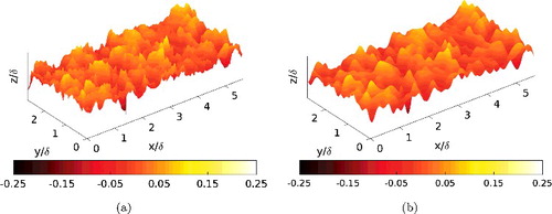
It is essential to choose an appropriate value for the cut-off wavenumber k_c, all wavenumbers above which are filtered out. If k_c is too low, the filtered data will be too smooth and will not be an accurate representation of the original data. If it is too high, a lot of small and aerodynamically irrelevant scales would be present in the data which would significantly increase the computational cost. The value of k_c depends to a great extent on the topography of the rough surface and hence no general recommendations can be given. However, studies conducted by Busse et al. [24] on one of the samples considered in the present work showed that a difference of 8% between the filtered and unfiltered values of the average and rms roughness height, S_a and S_q, retained most of the large-scale surface topography. The same criterion is used in the present work to determine k_c whose value is adjusted accordingly depending on the sample. Once k_c and the domain size are specified, the periodic sample is a precisely defined representation of the original surface and can be used together with DNS in a rigorous manner.

2.2. Geometry, boundary conditions and meshing criteria for DNS

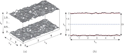
The rough surface samples are used as no-slip wall boundaries in incompressible turbulent channel flow. The streamwise, spanwise and wall-normal directions in the computational domain are denoted by x, y and z, respectively, with corresponding domain lengths L_x, L_y and L_z. Considering the cut-off wavenumber criterion mentioned in the previous section in conjunction with the streamwise domain length, the maximum streamwise wavenumber is given by k_cL_x. The samples have an aspect ratio of 2:1, which means L_x = 2L_y. The rough surface on the upper boundary corresponds to a mirror image of that on the lower boundary but translated by L_x/2 and L_y/2 in the streamwise and spanwise directions, respectively. The mean surface height is set as the mean reference plane, z = 0 at the bottom boundary and z = 2δ at the top boundary, where δ is the channel half-height. The channel height of 2δ is measured as the distance between the bottom and top mean reference planes. The domain length in the wall-normal direction, L_z, is slightly larger than 2δ to take into account the height of the roughness features. Figure 3 shows a schematic representation of the computational domain. The friction Reynolds number for this study is Re_τ = δu_τ/ν = 180, where u_τ is the friction velocity of the fluid, for which the flow is in the transitionally rough regime and where DNS is feasible for large number of samples. All rough surface samples are scaled to the same roughness height, k, defined for this study by the mean peak-to-valley height, S_{z, 5 × 5} (refer Appendix 1 for definition), such that k = δ/6. It has been recommended that in order to study universal roughness behaviour, k should be small compared to δ. Jiménez [9] recommends δ/k in excess of 40. In order to achieve a significant roughness effect for δ/k > 40, very high Re_τ, in excess of 1000, would be required. This in turn would lead to extremely dense meshes as the small scales of motion, especially close to the rough walls, would need to be resolved. These factors lead to a prohibitively high computational cost. Hence, δ/k = 6 is used, which leads to a clear roughness effect at Re_τ = 180. This is discussed in Section 4. Also discussed in Section 4 is the effect of the relatively low δ/k within the context of outer layer similarity.

Figure 3. Schematic representation of the computational domain. (a) 3D view (the scale of the surfaces has been increased in the wall-normal direction for clarity); (b) view in the x–z plane. The dashed lines represent the bottom and top mean reference planes and the dash-dot line represents the channel centreline.

Uniform grid spacing is used in the streamwise and spanwise directions, taking the minimum of the following two criteria: Δx⁺ = Δy⁺ ≈ 5 (‘+’ superscripts indicate wall-units) and Δx = Δy ≈ λ_min/12, where Δx and Δy are the streamwise and spanwise grid spacings and λ_min is the smallest wavelength of the rough surface after filtering, defined as the inverse of the filter cut-off wavenumber, k_c. A stretched grid is used in the wall-normal direction. In the region of the roughness features, min(h(x, y)) < z < max(h(x, y)), uniform grid spacing is used with Δz⁺_min < 1 and gradual stretching is applied towards the channel centre with Δz⁺_max ⩽ 5. The grid resolution has been validated in Busse et al. [24] on the basis of a grid refinement study.

The three-dimensional, incompressible Navier–Stokes equations, non-dimensionalised by δ and u_τ, are discretised using a standard second-order central difference scheme in the spatial domain which operates on a staggered cartesian grid and use a second-order Adams–Bashforth method for temporal discretisation. The flow is driven by a constant mean streamwise pressure gradient, which fixes the value of the friction velocity, , where ρ is the fluid density and dP/dx is the mean streamwise pressure gradient. An immersed boundary method, described in detail in Busse et al. [24], is used to resolve the rough walls.

3. Surface samples and topographical properties

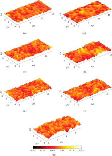
Flow over a total of 17 rough surface samples has been simulated. The database includes two carbon–carbon composite surfaces, a concrete surface, a graphite surface, as well as surfaces subject to the processes of casting, hand filing (two cases), gritblasting, grinding, shotblasting, spark-erosion (five cases) and replicas of two ship propeller surfaces eroded by periods of service. In order to simplify naming, samples are assigned names as given in Table 1. These are the names used henceforth. The composite and graphite samples were exposed to arc-heating in order to simulate the environment experienced by space vehicles while re-entering the atmosphere. The cast, filed, gritblasted, ground, ship propeller, shotblasted and one out of the five spark-eroded samples (spark-eroded_5 from Table 1) were taken from standard roughness comparators. The remaining four spark-eroded samples were taken from a spark-eroded surface provided by an industrial third-party. These four samples along with the ship propeller samples were selected as different sub-sections from the same respective larger rough surface scan. The concrete sample was taken from a larger block of concrete. Surface plots of all 17 rough surfaces are shown in Appendix 2. The composite and filed samples have strong directional alignment of their roughness features. In order to study this phenomenon, two samples of each are evaluated; one having features aligned in the streamwise direction and the other having features aligned in the spanwise direction. In Appendix 2, Figure B1(b,c) shows the composite samples, s2 and s3, with features aligned in the streamwise and spanwise directions, respectively, and Figure B1(e,f) shows the filed samples, s5 and s6, with features aligned in the spanwise and streamwise directions, respectively. The ground sample, s9, also shows strong directional alignment of features in the spanwise direction, as shown in Figure B1(i).

Table 1. Rough surface sample naming convention.

Sample	Type
s1	cast
s2	composite_1
s3	composite_2
s4	concrete
s5	filed_1
s6	filed_2
s7	graphite
s8	gritblasted
s9	ground
s10	ship-propeller_1
s11	ship-propeller_2
s12	shotblasted
s13	spark-eroded_1
s14	spark-eroded_2
s15	spark-eroded_3
s16	spark-eroded_4
s17	spark-eroded_5

A large number of parameters [27] can be used to characterise rough surfaces. Table 2 displays a broad list of parameters for the current dataset of 17 samples, whose description and computation is given in Appendix 1. These parameters are computed for the filtered surface samples. Flack and Schultz [17] mention that skewness, S_sk, is a quantitative way of describing whether a rough surface has more pronounced peaks or valleys. A negative value of skewness indicates that the surface is pitted, for example, due to corrosion or surface wear, whereas a positive value indicates roughness due to isolated large peaks, for example, due to deposition of foreign materials (as in biological fouling). A surface skewness value close to zero indicates a more or less homogenous distribution of peaks and valleys. The s1, s2, s7, s14 and s15 samples have a positive value for skewness, whereas all other samples have a negative value. Also, s15 has a skewness value close to zero.

Table 2. Topographical properties of the rough surface samples in this study. S_{z, 5 × 5} = δ/6, k_cL_x = maximum streamwise wavenumber. All length scales are non-dimensionalised by the mean channel half-height, δ. and α_rms are computed in degrees. Refer Appendix 1 for a description of each property and its calculation. Surface sample naming convention described in Table 1.

Property	s1	s2	s3	s4	s5	s6	s7	s8	s9	s10	s11	s12	s13	s14	s15	s16	s17
kcLx	24	24	24	28	36	32	24	24	18	36	20	18	24	24	24	24	18
Sa	0.0304	0.0353	0.0323	0.0304	0.0243	0.0353	0.0294	0.0275	0.0412	0.0257	0.0274	0.0321	0.0312	0.0351	0.0284	0.0294	0.0308
Sq	0.0387	0.0436	0.0409	0.0379	0.0319	0.0427	0.0373	0.0358	0.0509	0.0328	0.0358	0.0409	0.0396	0.0441	0.0361	0.0372	0.0383
Ssk	0.5964	0.2434	−0.1852	−0.0531	−0.3686	−0.4132	0.2797	−0.5190	−0.1329	−0.2315	−0.4334	−0.4081	−0.3048	0.4355	0.0451	−0.1653	−0.3881
Sku	4.006	2.869	3.012	2.708	3.912	2.514	2.974	3.844	2.817	3.504	4.430	3.379	3.394	3.626	3.229	3.101	2.871
Sz, max	0.2949	0.3017	0.2644	0.2263	0.2622	0.2626	0.2290	0.2621	0.2660	0.2818	0.3147	0.2610	0.3185	0.3864	0.2674	0.2659	0.2314
L^corx	0.5347	2.0128	0.4676	0.2222	0.1786	11.2700	0.2139	0.2160	0.9450	0.7014	0.5192	0.9825	0.9912	1.5172	0.8190	0.6893	0.2808
L^cory	0.5131	0.5611	2.1821	0.1968	5.352	0.3886	0.3509	0.2958	11.6000	1.0971	1.0171	0.9211	1.3759	1.2848	0.4998	0.6471	0.3574
Ssl	0.5962	2.0174	2.1894	0.3507	5.352	11.2700	0.3591	0.3351	11.6000	1.4636	1.0727	1.0115	1.7411	1.7041	0.8357	0.8324	0.3613
Sal	0.4670	0.5748	0.4670	0.1871	0.1883	0.3890	0.2181	0.2153	0.9454	0.6019	0.5246	0.9361	0.9015	1.1952	0.5051	0.6001	0.2798
Str	0.7833	0.2849	0.2133	0.5336	0.0701	0.0688	0.6074	0.6427	0.1606	0.4112	0.4890	0.9255	0.5178	0.7014	0.6044	0.7219	0.7745
S^flowtr	0.9595	0.2857	4.6666	0.8696	29.9664	0.0345	1.6364	1.3695	11.7172	1.5641	1.9591	0.9400	1.3762	0.8468	0.6102	0.9388	1.2728
ESx	0.1098	0.0952	0.1418	0.3177	0.2194	0.0745	0.2798	0.2339	0.0710	0.1325	0.0877	0.0600	0.1057	0.1170	0.1000	0.1048	0.1781
ESy	0.1162	0.1425	0.0963	0.3071	0.0990	0.1998	0.2791	0.2242	0.0105	0.1067	0.0583	0.0611	0.1062	0.1060	0.1133	0.1082	0.1465
S	84.50	48.02	43.62	12.10	57.28	63.51	13.78	15.85	269.12	90.86	126.12	153.12	88.45	60.50	77.88	79.96	29.29
Sf	4.644	2.293	3.100	1.928	6.297	2.370	1.934	1.856	9.590	6.028	5.541	4.601	4.684	3.548	3.901	4.201	2.612
Sw	42.940	24.290	24.261	6.887	30.840	32.210	7.709	8.580	131.620	46.051	64.418	75.630	44.530	30.630	40.180	41.190	15.310
Sf/S	0.0550	0.0477	0.0711	0.1593	0.1099	0.0373	0.1406	0.1171	0.0356	0.0663	0.0439	0.0300	0.0530	0.0586	0.0501	0.0525	0.0892
Sw/S	0.5082	0.5057	0.5562	0.5682	0.5383	0.5072	0.5594	0.5414	0.4891	0.5069	0.5108	0.4939	0.5035	0.5062	0.5194	0.5151	0.5225
Λs	639	914	378	48	116	1830	65	99	1854	390	1153	2934	693	537	838	734	190
	6.245	5.493	7.357	16.801	11.711	4.213	14.913	12.674	4.167	7.521	4.937	3.494	6.070	6.663	5.616	5.871	9.861
αrms	7.833	7.249	9.176	20.662	14.610	5.425	18.388	15.894	5.348	9.607	6.196	4.448	7.736	8.579	7.009	7.542	12.333

The data shown in Tables 2 and 3 and roughness height maps for the 17 surfaces after filtering are available in .csv format at http://dx.doi.org/10.5258/SOTON/392562

The largest correlation lengths are exhibited by s5 and s6 in their respective spanwise and streamwise directions. This is attributed to the strong anisotropy of their roughness features. The directionality of the features of a given rough surface sample can be obtained from the surface texture aspect ratio, S_tr, which is given by the ratio of the shortest-to-longest correlation lengths of the sample. If S_tr > 0.5, then the sample is regarded as statistically isotropic, whereas anisotropic samples have S_tr < 0.3 (refer [27]). All samples, with the exception of s2, s3, s5, s6, s9 and s10, have S_tr > 0.5 and hence are statistically isotropic. The s10 sample has S_tr = 0.41 and can be considered weakly anisotropic. Both the composite samples, s2 and s3, are anisotropic with S_tr = 0.28 for s2 and its dominant features oriented in the streamwise direction and S_tr = 0.21 for s3 with its dominant features oriented in the spanwise direction.

A parameter called the flow texture ratio, , has been defined as the ratio of sample spanwise-to-streamwise correlation lengths, (refer Appendix 1 for definitions). This parameter is another indicator of the anisotropy of the roughness features. If , for example, for the s5 sample, its roughness features have strong directional preference in the spanwise direction (refer Figure B1(e)) and if , for example, for the s6 sample, its roughness features have strong directional preference in the streamwise direction (refer Figure B1(f)).

The effective slope, ES, as introduced by Napoli et al. [28], represents the overall gradient of the roughness elements of an irregular rough surface. Higher values of ES indicate more dense roughness whereas lower values are obtained for relatively sparse roughness. In the case of three-dimensional roughness, the effective slope is computed in the streamwise and spanwise directions and denoted by ES_x and ES_y, respectively. Most samples have similar values of ES_x and similar values of ES_y. Based on these values, s4, s7 and s8 can be considered relatively more densely rough, whereas s9, s11 and s12 can be considered relatively sparsely rough. A closer look at the values of S_f/S and ES_x from Table 2 shows that 2 × S_f/S ≈ ES_x for the current dataset. This relation was also pointed out by Napoli et al. [28] in their studies. Figure 4(a) shows a plot of the two quantities and clearly establishes this relationship as all points fall on the straight line given by 2 × S_f/S = ES_x. Figure 4(b) shows the variation of Λ_s with ES_x and a clear dependence is seen for these two quantities as well. This dependence seems sensible as S_f/S is an integral part of Λ_s.

Figure 4. (a) Variation of S_f/S with ES_x. The 2 × S_f/S = ES_x straight line is also shown; (b) variation of Λ_s with ES_x.

Bons [16] mentions that the mean streamwise forward-facing surface angle, , is geometrically related to the Sigal–Danberg parameter. This can be seen from Figure 5(a), which shows a semilogarithmic plot of the two quantities for the samples in this study. From this, it is logical to follow that S_f/S is also related to (Figure 5(b)). This serves as motivation to also look at the variation of the root-mean-square of the streamwise surface angle, α_rms, with Λ_s (Figure 5(c)) and with S_f/S (Figure 5(d)). These relationships also confirm that the streamwise forward-facing surface angle is approximately linearly related to the frontal area of the roughness elements. α_rms was proposed by [2] as an important parameter characterising real roughness in the context of turbine blades. It is also worth noting that , the tangent of the mean streamwise forward-facing surface angle approximately represents the streamwise effective slope.

Figure 5. (a) and (b) Variation of Λ_s and S_f/S with (degrees); (c) and (d) variation of Λ_s and S_f/S with α_rms (degrees).

The above observations establish that ES_x, and α_rms are all closely linked to the solidity, S_f/S for the current set of samples and as such cannot be regarded as independent parameters. This is particularly important for the parametric-fitting studies conducted in Section 5 as, if one of the four properties enters the fit at a certain stage, none of the other three would provide any more useful information at a later stage. Refer Section 5 for further details.

4. Simulation parameters and results

The streamwise, spanwise and wall-normal domain lengths for all samples along with number of grid cells in each direction and the grid spacing are displayed in Table 3. Δz⁺_max is the maximum wall-normal grid spacing at the channel centre. The large variation in the streamwise and spanwise domain extents is seen due to the fact that the roughness height for all samples is maintained the same, at k = δ/6 (where k = S_{z, 5 × 5}). All simulations are performed at Re_τ = 180, for which the roughness Reynolds number, k⁺ = ku_τ/ν = 30. Corresponding parameters for the smooth-wall reference case are as follows: L_x/δ = 12, L_y/δ = 6, L_z/δ = 2, n_x = 256, n_y = 256, n_z = 224, Δx⁺ = 8.4375, Δy⁺ = 4.2188, Δz⁺_max = 4.70, mean streamwise velocity, and centreline velocity, U_c/u_τ = 18.44.

Table 3. Rough surface sample domain sizes , non-dimensionalised by δ, number of grid cells and grid spacings, for the samples in this study. n_x, n_y and n_z are the number of grid cells in the streamwise, spanwise and wall-normal directions, respectively. Also shown are the values of ΔU⁺ and peak profile TKE.

Sample	Lx/δ	Ly/δ	Lz/δ	nx	ny	nz	Δx^+, Δy^+	Δz^+max	ΔU^+	Peak TKE
s1	13.00	6.50	2.236	480	240	272	4.8750	4.74	3.39	3.05
s2	9.80	4.90	2.290	384	192	288	4.5938	4.16	2.72	3.10
s3	9.34	4.67	2.287	384	192	288	4.3781	3.65	3.94	3.04
s4	4.92	2.46	2.238	384	192	256	2.3063	4.14	4.95	2.97
s5	10.70	5.35	2.298	448	224	288	4.3007	3.62	4.17	3.11
s6	11.27	5.64	2.292	448	224	288	4.5281	3.66	1.28	3.47
s7	5.25	2.63	2.232	384	192	256	2.4609	4.13	5.02	2.88
s8	5.63	2.82	2.324	320	160	288	3.1669	3.72	4.36	3.06
s9	23.20	11.60	2.292	768	384	256	5.4375	5.06	2.63	3.29
s10	13.48	6.74	2.342	512	256	288	4.7391	4.07	2.84	3.36
s11	15.88	7.94	2.387	576	288	288	4.9631	4.86	2.57	3.95
s12	17.50	8.75	2.308	640	320	256	4.9219	5.02	1.71	3.45
s13	13.30	6.65	2.388	512	256	288	4.6758	4.82	2.82	3.27
s14	11.00	5.50	2.300	512	256	320	3.8672	3.48	3.42	3.00
s15	12.48	6.24	2.248	512	256	288	4.3875	3.58	2.67	3.26
s16	12.65	6.32	2.300	512	256	288	4.4459	3.71	2.77	3.22
s17	7.65	3.83	2.282	320	160	256	4.3054	4.40	4.36	3.33

The data shown in Tables 2 and 3 and roughness height maps for the 17 surfaces after filtering are available in .csv format at http://dx.doi.org/10.5258/SOTON/392562

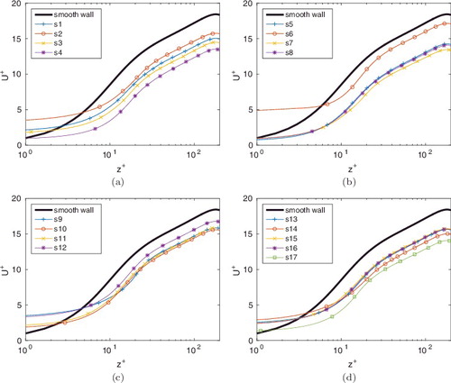
Time-averaged mean streamwise velocity profiles in wall-units against the wall-normal distance are shown in Figure 6(a–d) on semilogarithmic axes. Smooth-wall profiles have also been shown for comparison. The roughness function, ΔU⁺, is generally measured as the downward shift of the log region for a given rough-wall profile from the corresponding smooth-wall profile. However, due to the low Reynolds number in this study, no clearly defined log region is present. Thus, ΔU⁺ is computed by subtracting the centreline velocity for a given rough surface simulation from the corresponding smooth-wall centreline velocity [29]. ΔU⁺ values for all samples are given in Table 3. A significant roughness effect is seen for all samples, from the downward shift in the mean velocity profiles. There is a wide range, from ΔU⁺ = 1.28 (s6 sample) to ΔU⁺ = 5.02 (s7 sample), despite all samples being scaled to the same roughness height. This is a clear indication that the roughness function depends not only on the roughness height for a given sample but also on its detailed roughness topography. The s6 sample has the smallest roughness function value at ΔU⁺ = 1.28. This is because the roughness features of this sample are strongly aligned in the streamwise direction (refer Figure B1(f)) and this anisotropic topography gives less resistance to the flow. This leads to a comparatively lower increase in surface friction and hence a smaller value of ΔU⁺ compared to other samples. The s7, s4 and s8 samples show some of the largest values of ΔU⁺, at 5.02, 4.95 and 4.36, respectively. This closeness in ΔU⁺ values is possibly due to similar values of some of their surface properties; for example, L^cor_x, S_f and Λ_s (refer Table 2). The ship-propeller samples, s10 and s11, also exhibit similar values of ΔU⁺, despite their surface properties showing numerous differences.

Figure 6. Mean streamwise velocity profiles for the 17 rough surface samples. U⁺ = u/u_τ is the mean streamwise velocity in wall-units and z⁺ = zu_τ/ν is wall-normal distance in wall-units.

The variation of ΔU⁺ with the effective slope is shown in Figure 7, where it is seen that ΔU⁺ increases with ES_x. This general dependence of ΔU⁺ on the effective slope indicates that the current set of samples lies in the waviness regime (described by [23]). The curve appears to be levelling out at higher values of ES_x, implying that the critical ES_x separating the waviness and roughness regimes may be close to these values. The variation of ΔU⁺ with Λ_s is shown in Figure 8 on a semilogarithmic plot. It can be seen that ΔU⁺ decreases as Λ_s increases. The plot also shows a good collapse of the data, with the coefficient of determination, R² = 0.8836 and rms error of the fit, σ = 0.3753. Several parameters such as the roughness density, shape and direction with respect to the mean flow are taken into account while computing Λ_s and the data already scales very well with the roughness function. This serves as an initial motivation to perform a more methodical study of surface properties that influence ΔU⁺, as described in Section 5.

Figure 7. ΔU⁺ against ES_x for the 17 samples.

Figure 8. ΔU⁺ against Λ_s for the 17 samples. The black solid line shows the linear least squares fit to the data.

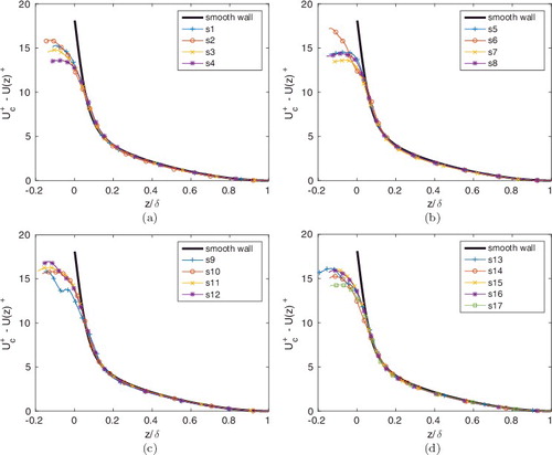
The time-averaged mean streamwise velocity defect profiles for the samples are shown in Figure 9(a–d). U(z)⁺ denotes the temporally and spatially averaged streamwise velocity profiles in the wall-normal direction in wall-units. The centreline velocity, U⁺_c, is obtained at z = δ. The profiles are then computed by taking the difference between the two, U⁺_c − U(z)⁺, for each wall-normal location. They are plotted against the wall-normal distance normalised by the channel half-height, z/δ. The region where these profiles widely differ from each other for the different samples is close to the roughness features. This is seen from the plots for z/δ⪅0.1. Beyond this region and closer to the channel centre, the profiles follow the smooth-wall data to a good degree, thus obtaining a good collapse. This indicates that outer layer similarity is preserved and Townsend's wall similarity hypothesis [30] is satisfied. An important observation from this study is that outer layer similarity for the irregular rough samples is achieved despite the relatively low Re_τ and ratio of channel half-height to roughness height of δ/k = 6.

Figure 9. Mean streamwise velocity defect profiles for the 17 rough surface samples. U⁺_c = u_c/u_τ is the mean streamwise centreline velocity in wall-units, U(z)⁺ = u(z)/u_τ are the mean streamwise velocity profile values and z/δ = wall-normal distance.

Profiles of the turbulent kinetic energy (TKE) in wall-units, given by , are shown in Figure 10(a–d), plotted against the wall-normal distance, along with corresponding smooth-wall profiles. Additionally, Figure 11 shows profiles of streamwise, , spanwise, and wall-normal, fluctuations for the smooth-wall case and the s8 sample as an example. This figure enables us to see graphically the contribution of each to the TKE. It is clear from the figure that peak streamwise fluctuations are higher in magnitude than both the peak spanwise and peak wall-normal fluctuations for the smooth-wall as well as the s8 sample. Also, the smooth-wall peak streamwise fluctuations are higher than the s8 peak streamwise fluctuations. The above two observations were found to be true for all rough surface samples in this study. To quantify the anisotropy of the velocity fluctuations and hence TKE, the diagonal components of the normalised Reynolds stress anisotropy tensor, where δ_{i, j} is the Kronecker delta, are computed at the peak value of TKE for all samples. Since it is known that −1/3 ≤ b_{i, j} ≤ 2/3, a component with positive value of b_{i, j} indicates a dominant contribution towards TKE. All samples exhibit 0.39 < b_{1, 1} < 0.49, with −0.20 < b_{2, 2} < −0.13 and −0.29 < b_{3, 3} < −0.25 (compared to the smooth-wall values, b_{1, 1} = 0.53, b_{2, 2} = −0.22 and b_{3, 3} = −0.31), which implies that streamwise fluctuations still have the dominant contribution to TKE, although the anisotropy is reduced relative to the smooth wall.

Figure 10. Turbulent kinetic energy profiles for the 17 rough surface samples. z/δ = wall-normal distance.

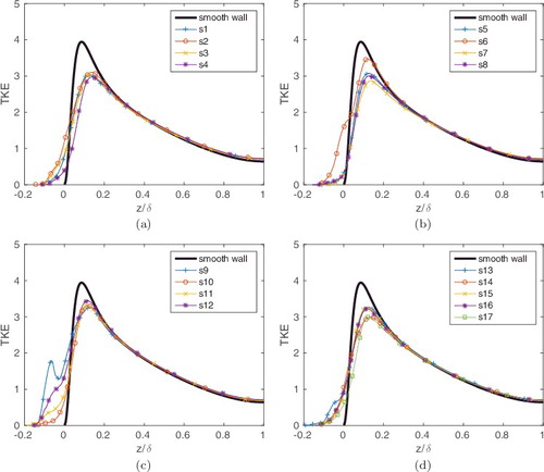
Figure 11. Profiles of , and for the smooth-wall case and s8 sample.

In general, an increased amount of roughness is accompanied by a decrease in the peak streamwise fluctuations [29,31,32], which means samples with higher peak magnitudes have lower ΔU⁺ compared to samples with lower peak magnitudes. This influences TKE as well, as samples with higher ΔU⁺ show a lower value of peak TKE (refer Table 3). Within the region of the roughness features and close to z/δ ≈ 0, all samples show TKE values greater than the smooth-wall value. The reason is that rough-wall velocity fluctuations can occur very close to the roughness features, including at and below the mean wall location, z/δ = 0. This is not possible in the case of smooth walls. In general, an increase in TKE is observed close to the rough walls, whereas a collapse with the smooth-wall data is seen away from the walls. For the smooth-wall case, the TKE peak is located at z/δ ≈ 0.1, whereas rough-wall peaks for all samples are located slightly above that.

5. Parametrisation of topographical properties for ΔU⁺ and TKE

Although a general solution to the roughness problem must be delayed until a more complete dataset is available for fully rough cases and including a wider Reynolds number range, it seems sensible to try to make as much progress as possible with the present set of restricted data, first of all to find out the issues that arise in formulating a general empirical model and, second, to guide the next set of simulations to best exploit the available computational resources. As can be seen from Table 3, there is a large variation in the roughness function ΔU⁺ that must be due to other parameters, besides the height, that govern the surface topography. To obtain surface properties that possibly influence the roughness function, a fitting process is employed whereby ΔU⁺ is plotted against a combination of surface properties and the quality of the fit is improved by successively adding other properties. Additions are made based on a systematic testing of all available properties using specific mathematical forms (algebraic, exponential, logarithmic or power) and selecting the property and form that gives the best possible fit. In Table 4, all forms tried for this process are listed for an example surface property, p. The particular form for a property may not necessarily be optimal, since only the above-mentioned four mathematical forms are tested and there may be other forms which might influence the fitting process. Combinations of surface parameters are denoted by λ_n, where n = 0 for a baseline model, n = 1 for a 1-parameter model and so on. An example for n = 2 could be where c₁ and c₂ are fitting constants.

Table 4. Mathematical forms of properties tested during the fitting process. c is a fitting constant and p is the value of a given surface property.

Name of form	Algebraic	Exponential	Logarithmic	Power
Equation of form	1 + (c · p)	e^c · p	1 + c · ln (p)	p^c

To measure the success of the method, we use the root-mean-square error, σ, between the data and a straight-line curve fit using the derived parameter, as well as the value of the coefficient of determination, R² of the fit. In order to maximise the number of property combinations tested, fits giving the three lowest values of σ (which means the three highest values of R²) are retained for further improvement. This means, for example, in case of n = 0 (or the baseline) model, where ΔU⁺ is fitted with a single surface property, fits of those properties which obtain the three lowest values of σ are selected for further improvement by addition of more properties. However, in the following description, only the best fits are reported. The reason for selecting multiple property combinations is also because a given property combination that gives the lowest value of σ for n = 1, for example, may not necessarily give the lowest σ value for n = 2 because of the interactions between different surface properties. Parameters are continued to be added until no significant improvement of the fit is obtained and the fit with the final lowest value of σ is selected as the best.

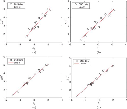
For n = 0 to fit ΔU⁺, we consider the performance of a solidity parameter, expressed here in logarithmic form, (9) Using just this parameter, the best fit to the data is ΔU⁺ = aλ₀ + b, with a = 2.0438 and b = 8.9035 and with σ = 0.3807 and R² = 0.8802. The resulting straight line is plotted in Figure 12(a) and already a reasonable fit to the data can be seen. Given the success of the simplest measure, our strategy is to introduce modifications to the definition of λ₀ based on additional surface properties as shown in Table 2.

Figure 12. Linear fits to the DNS data, correlating the roughness function, ΔU⁺ with different parameters λ₀, λ₁, λ₂ and λ₃, corresponding to Equations (9(9) ), (11(11) ), (12(12) ) and (13(13) ).

Extensions to the solidity parameter have already appeared in the literature and, for irregular surfaces, van Rij et al. [15] redefined the parameter introduced by Sigal and Danberg [14], previously given in Equation (4(4) ). A generalisation of this approach is to set (10) where S_w is the wetted area of the forward-facing elements of the surface and Sigal and Danberg used β = 1.6 (note that Sigal and Danberg used the inverse of this parameter, whereas we prefer a definition where λ can be interpreted as the solidity or density of the roughness). However, using this value of β in the present study led to no improvement in the standard error. A separate exercise was undertaken to optimise the value of the exponent, giving β = 0.18, but with a barely measurable increase in R². The reasons for the failure of this additional term are clear from Table 2, since for the types of roughnesses considered, the wetted area parameter is always about half of the planform area, i.e. there is an approximate symmetry (of forward-facing and rearward-facing roughness elements) in the roughness samples. Thus, the term S_f/S_w introduces no additional useful information. One could continue using (10(10) ) as the reference parameter and get the same results, but we prefer only to use parameters that are justified by the data and instead revert to the simple solidity, λ₀, as our baseline property.

The next step is to test each of the potential surface parameters as modifications to λ₀. The best two, with almost identical performance, were the streamwise correlation length parameter and the flow texture ratio . The success of both suggests that the spanwise correlation length is less important and we retain the best-performing parameter, with a single optimised coefficient for n = 1 to give (11) The improved fit to the data is shown in Figure 12(b), with σ = 0.3073 and R² = 0.9220. It is interesting that a streamwise correlation length enters as the next most important parameter after the solidity since this type of parameter does not appear in many correlations. The parameter is additionally intriguing since dense roughness cases will have low values of , and from the correlation, this would lead to lower λ₁ and hence lower ΔU⁺, which is indeed what is observed [9]. The absence of dense roughness cases (S_f/S > 0.15) from the current sample set means that we cannot test this fully, and addressing this point would be a priority for future simulations.

We continue the process to define the best models for n = 2 and 3. The best model for n = 2 is found to include the relative rms roughness height parameter, S_q, as (12) with σ = 0.1806 and R² = 0.9731. The best model for n = 3 includes the skewness, S_sk, as (13) with σ = 0.1383 and R² = 0.9842. Figure 12(c,d) shows the continued improvements seen with the λ₂ and λ₃ representations. The largest remaining errors in the fit to the data are less than 0.1u_τ. Additional parameters were tested, but with no significant further improvements found. Fit parameters for λ₀, λ₁, λ₂ and λ₃ are summarised in Table 5. Tests were also run by removing parameters individually, confirming that a ranking in order of importance is (1) solidity, (2) streamwise correlation length non-dimensionalised by the mean peak-to-valley height, (3) rms roughness height non-dimensionalised by the mean peak-to-valley height and (4) skewness. Note that the roughness height is not one of these parameters since all the cases were run for the same S_{z, 5 × 5}. Had the simulations been in the fully rough regime, the equivalent sand-grain roughness k⁺_{s, eq} would be determined as a constant (dependent on all the above parameters) multiplied by some suitable measure of the roughness height, e.g. S⁺_q or S⁺_{z, 5 × 5}. Both rms roughness height and skewness are part of the Flack and Schultz model [17], and hence it is no surprise to see them here. Also, as we have seen, the effective slope, mean and rms streamwise forward-facing surface angles are proportional to the solidity for these surfaces, and hence cannot be considered as independent parameters.

Table 5. Best fit parameters for λ₀, λ₁, λ₂ and λ₃, corresponding to Equations (9(9) ), (11(11) ), (12(12) ) and (13(13) ). ΔU⁺ = aλ_n + b, where a = slope of the fit and b = y-axis intercept. σ = rms error of the fit and R² = coefficient of determination.

Parameter	a	b	σ	R^2
λ0	2.0438	8.9035	0.3807	0.8802
λ1	1.4988	7.8221	0.3073	0.9220
λ2	1.5150	8.1607	0.1806	0.9731
λ3	1.4699	8.0394	0.1383	0.9842

We should caution that the above analysis is only the first step. As more samples are added covering different types of roughnesses (dense, for example), we might expect that additional parameters would be required. What is important is that we now have a systematic method to incorporate additional parameters. We caution again that the models in Equations (9(9) )–(13(13) ) should not be used for k⁺_{s, eq} since the current data were all taken in the transitionally rough regime. What we have been able to do is identify a number of parameters that contribute significantly to the roughness function in this regime and it is likely that the same parameters contribute to the determination of k⁺_{s, eq}. The same numerical coefficients would only be found if all the samples followed the same path through the transitionally rough regime, which is unlikely.

A similar approach as above was also utilised to fit surface property data to the value of peak TKE from Table 3. Different parameters are seen to appear in the model as the fluctuations behave differently with property combinations as compared to ΔU⁺. The various models obtained for this process are given below.

n = 0: (14) n = 1: (15) n = 2: (16) n = 3: (17)

The fits for the above models are shown in Figure 13(a–d) and fit parameters are summarised in Table 6. Although fits are reported only up to n = 3, further improvements, following the same systematic fitting approach as described for ΔU⁺, are seen up to n = 5. Values up to σ = 0.0244 and R² = 0.9820 are obtained when the average roughness height, S_a, in its algebraic form and shortest correlation length, S_al, in its power form (both properties non-dimensionalised by S_{z, 5 × 5}) are included in the model. However, due to the relatively small size of the sample database for fitting purposes, the influence of these properties is probably not as significant as the ones seen up to n = 3. For n < 3, property combinations other than Equations (15(15) ) and (16(16) ) may give lower values of σ. But since (15(15) ) and (16(16) ) finally lead to Equation (17(17) ), which ultimately gives the lowest σ value of all final fits tested, it is selected as the best fit and is discussed here. The baseline parameter is the mean forward-facing surface angle, , which is an angle parameter as opposed to S_f/S, which is an area parameter, seen in the case of ΔU⁺. However, it has been shown in Figure 5(b) that S_f/S and are approximately linearly related.

Figure 13. Linear fits to the DNS data, correlating the peak TKE, with different parameters λ₀, λ₁, λ₂ and λ₃ corresponding to Equations (14(14) )–(17(17) ).

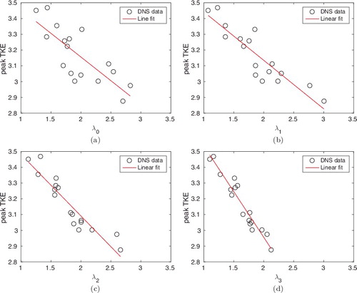
Table 6. Best fit parameters for λ₀, λ₁, λ₂ and λ₃, corresponding with Equations (14(14) )–(17(17) ). Peak TKE =aλ_n + b, where a = slope of the fit and b = y-axis intercept. σ = rms error of the fit and R² = coefficient of determination.

Parameter	a	b	σ	R^2
λ0	−0.3004	3.7568	0.1897	0.6169
λ1	−0.3074	3.7498	0.0966	0.8048
λ2	−0.3901	3.8716	0.0653	0.8681
λ3	−0.5765	4.1149	0.0352	0.9288

Also, it is understood that higher values of correspond to a higher roughness effect (from higher values of ΔU⁺, refer Tables 2 and 3) and hence its influence on the fluctuations would be significant. Other baseline parameters that gave σ values comparable to include α_rms, S_f/S, and ES_x, all in logarithmic form. This is not too surprising as the four parameters are interrelated. Surface skewness, S_sk, is the next important parameter and after that comes the rms roughness height non-dimensionalised by the mean peak-to-valley-height, S_q/S_{z, 5 × 5}, both of which also appear in λ₁ and λ₂, respectively, for the other baseline parameters, albeit in different forms. Spanwise effective slope, ES_y, is the next parameter to enter the fit, the appearance of which could relate to how the streamwise flow navigates around roughness features. It would be interesting in the future to understand why certain parameters enter the fit as opposed to others, which is not considered in this study. The baseline TKE fit is not as good as the fit for ΔU⁺ but significant improvement is seen until λ₃. A separate fitting study conducted for the profile peak streamwise fluctuations, alone also gave the same properties influencing the fit, although in a slightly different order.

6. Conclusions

A direct numerical simulation study of 17 industrially relevant rough surface samples with the same physical roughness height and at the same friction Reynolds number, in the transitionally rough regime, has been presented. Mean streamwise velocity profiles show a clear roughness effect for all samples. A wide range of the roughness function is obtained, from ΔU⁺ = 1.28 to 5.02, despite all samples being scaled to the same roughness height of k = S_{z, 5 × 5} = δ/6. It is thus clear that the roughness effect depends not only on the roughness height but also on the detailed roughness topography.

A process to determine which surface properties influence ΔU⁺ is then formulated. The process involves fitting the roughness function with one or more surface properties. Addition of properties to the model is based on a systematic testing of all available properties and selecting the combination that provides the best fit as measured by the value of root-mean-square error between the data and the fit as well as the coefficient of determination. A similar procedure is also applied to fit the profile peak turbulent kinetic energy. Optimised fits are developed for ΔU⁺ and peak TKE. Properties influencing ΔU⁺ include the solidity (S_f/S) and surface skewness (S_sk), which are known from literature, and, additionally, the streamwise correlation length (L^cor_x) and the rms roughness height (S_q). Properties influencing peak TKE are slightly different. The surface skewness and rms roughness height are still seen in the TKE fits together with the mean forward-facing surface angle () and spanwise effective slope (ES_y). The identification of key surface parameters that determine critical flow properties is an important conclusion of the current work. The final fits obtained for both ΔU⁺ and peak TKE are of high quality (with the value of R² = 0.9842 for ΔU⁺ and 0.9288 for TKE). Since all the simulation data were taken in the transitionally rough regime, this process is used only to determine the surface properties that influence ΔU⁺ and not predict an equivalent sand-grain roughness, which would require data in the fully rough regime. The process establishes that possibly the same properties would influence flow parameters in the fully rough regime as well. An extension of the procedure to the fully rough regime is straightforward but requires larger computational resources. Increasing the size of the data set by introducing more surfaces having different properties (for example, surfaces in the roughness regime with respect to their effective slope) would serve to increase the generality of the fitting process and could be considered a priority for future work.

Disclosure statement

No potential conflict of interest was reported by the authors.

Additional information

Funding

This work has been supported by the Engineering and Physical Sciences Research Council [grant number EP/I032576/1]. The UK Turbulence Consortium provided computing time on the ARCHER UK National Supercomputing service (http://www.archer.ac.uk) [grant number EP/L000261/1].

Appendices

Appendix 1. Parameters for the characterisation of rough surfaces

A large number of surface parameters are used to characterise the rough surfaces used in the current study. [27] gives a very extensive range of metrological parameters that may be used to describe rough surfaces in general. It is important to note that since the mean surface height is taken as the mean reference plane, z = 0, we get a relation for the mean surface height, as where h_{i, j} are roughness height values obtained after filtering and M, N are the number of data points in the streamwise and spanwise direction, respectively.

A.1 Amplitude parameters

Amplitude parameters are computed based on the distribution of roughness amplitude. The definition of roughness height considered in this study is the mean-peak-to-valley height, S_{z, 5 × 5}. To compute this quantity, a surface is first partitioned into 5 × 5 tiles of equal size and the maximum and minimum height for each of these tiles is computed. S_{z, 5 × 5} is then the difference between the mean of the maxima and mean of the minima. Other common measures for the roughness height of a surface are The maximum peak-to-valley height is given as Other amplitude parameters, which describe the shape of the rough surface, include,

A.2 Spacing parameters

Roughness spacing parameters characterise the spacing of the roughness features. They are computed from the areal autocorrelation function, The shortest correlation length is defined as and the longest correlation length is defined as The central lobe of the areal autocorrelation function is the simply connected area where R_h > 0.2 that contains (0, 0). The surface texture aspect ratio, S_tr, is given by the ratio of the shortest-to-longest correlation lengths, The surface correlation lengths are given as A parameter called the flow texture ratio, , which depends on the streamwise and spanwise correlation lengths, has been defined as

A.3 Aerodynamic parameters

In the context of aerodynamics, several other geometric parameters for the characterisation of rough surfaces have been defined. In the context of two-dimensional roughness, Napoli et al. [28] introduced the streamwise effective slope, ES. For three-dimensional surfaces, The solidity or frontal area ratio has been used extensively in literature and is an indication of the roughness density. It is given by the ratio of the total frontal area of all roughness elements to the planform area of the sample, S_f/S. The generalised Sigal–Danberg parameter as defined by van Rij et al. [15] is given as where S = L_xL_y is the planform area of the corresponding smooth surface. S_f is the total frontal area of all roughness elements and is given as Hence, S/S_f represents the inverse of the solidity. S_w is the total area of all roughness elements wetted by the flow, given as The function W(x, y) indicates whether or not a local infinitesimal surface element is wetted with respect to a given flow direction, . Since x is the streamwise direction in this study, .

For the definition of ES_x, ES_y and Λ_s, it has been assumed that an analytic and differentiable representation of the rough surface, h(x, y), is known, since the expressions then take a simpler form. The expressions from above can be reformulated for a discrete rough surface, h_{i, j}, by replacing the integrations with summations and using finite difference approximations for the derivatives.

Bons [16] defined a local streamwise forward-facing surface angle, denoted by α. Since a rough surface sample can be constructed as a series of streamwise traces of roughness height in the spanwise direction, the local streamwise forward-facing surface angle, α_j, is computed for each streamwise trace. For roughness elements facing the flow, where Δs is the streamwise spacing of the roughness elements. This relation is valid only for h_{j + 1} > h_j. The sum of all roughness elements having a definite value of α_j gives the total number of forward-facing roughness elements, n_f. The mean streamwise forward-facing surface angle, , is then given as and its root-mean-square value is given as

Appendix 2. Surface plots for the 17 rough surface samples

Surface height plots for the 17 rough surface samples in this study are shown in Figures B1 and B2. The scale of the plots has been increased in the wall-normal direction for clarity.

Figure B1. Surface plots for samples s1–s10. (a) s1, (b) s2, (c) s3, (d) s4, (e) s5, (f) s6, (g) s7, (h) s8, (i) s9, (j) s10. Plots shaded by roughness height. Refer Table 1 for naming convention. All plots have the same colourbar, shown at the bottom.

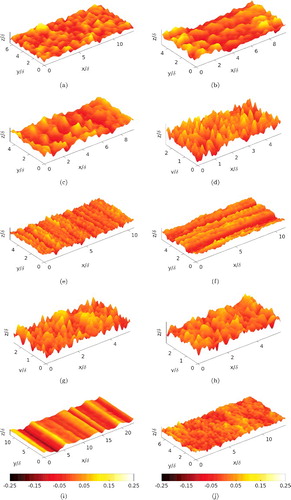
Figure B2. Surface plots for samples s11–s17. (a) s11, (b) s12, (c) s13, (d) s14, (e) s15, (f) s16, (g) s17. Plots shaded by roughness height. Refer Table 1 for naming convention. All plots have the same colourbar, shown at the bottom.

References

- Ligrani PM, Oliviera MM, Blaskovich T. Comparison of heat transfer augmentation techniques. AIAA J. 2003;41(3):337–362.
- Acharya M, Bornstein J, Escudier MP. Turbulent boundary layers on rough surfaces. Exp Fluids. 1986;4:33–47.
- Bons JP. St and cf augmentation for real turbine roughness with elevated freestream turbulence. Turbomach J. 2002;124(4):632–644.
- Kirschner CM, Brennan AB. Bio-inspired antifouling strategies. Annu Rev Mater Res. 2012;42:211–229.
- Townsin RL. The ship hull fouling penalty. Biofouling 2005;19:9–15.
- Wahl M. Marine epibiosis. I. Fouling and antifouling: some basic aspects. Mar Ecol Prog Ser. 1989;58:175–189.
- Arnfield AJ. Two decades of urban climate research: a review of turbulence, exchanges of energy and water and the urban heat island. Int J Climatol. 2003;23(1):1–26.
- Finnigan J. Turbulence in plant canopies. Annu Rev Fluid Mech. 2000;32:519–571.
- Jiménez J. Turbulent flows over rough walls. Annu Rev Fluid Mech. 2004;36:173–196.
- Nikuradse J. Laws of flow in rough pipes. VDI-Forchungsheft 361, Series B, Vol. 4. 1933. ( English translation NACA technical memorandum 1292, 1950).
- von Schlichting H. Experimental investigation of the problem of surface roughness. Ingenieur-Archiv. 1936;7(1). ( English translation NACA technical memorandum 823, 1937).
- Bradshaw P. A note on “critical roughness height” and “transitional roughness”. Phys Fluids. 2000;12(6):1611–1614.
- Sigal A, Danberg JE. Analysis of turbulent boundary-layer over rough surfaces with application to projectile aerodynamics. Aberdeen Proving Ground, Aberdeen (MD): U.S. Army Ballistic Research Laboratory; 1988. ( Technical report BRL-TR-2977).
- Sigal A, Danberg JE. New correlation of roughness density effects on the turbulent boundary layer. AIAA J. 1990;28(3):554–556.
- van Rij JA, Belnap BJ, Ligrani PM. Analysis and experiments on three-dimensional, irregular surface roughness. J Fluids Eng. 2002;124(3):671–677.
- Bons JP. A critical assessment of Reynolds analogy for turbine flows. J Heat Transfer. 2005;127:472–485.
- Flack KA, Schultz MP. Review of hydraulic roughness scales in the fully rough regime. J Fluids Eng. 2010;132:041203-1–041203-10.
- Musker AJ. Universal roughness functions for naturally occurring surfaces. Trans Can Soc Mech Eng. 1980;6(1):1–6.
- Waigh DR, Kind RJ. Improved aerodynamic characterization of regular three-dimensional roughness. AIAA J. 1998;36(6):1117–1119.
- Wieringa J. Representative roughness parameters for homogenous terrain. Boundary Layer Meteorol. 1993;63:323–363.
- Grimmond CSB, Oke TR. Aerodynamic properties of urban areas derived from analysis of surface form. J Appl Meteorol. 1998;38:1262–1292.
- Yuan J, Piomelli U. Estimation and prediction of the roughness function on realistic rough surfaces. J Turbul. 2014;15(6):350–365.
- Schultz MP, Flack KA. Turbulent boundary layers on a systematically varied rough wall. Phys Fluids 2009;21:015104-1–015104-9.
- Busse A, Lützner M, Sandham ND. Direct numerical simulation of turbulent flow over a rough surface based on a surface scan. Comput Fluids. 2015;116:129–147.
- Sherrington I, Howarth GW. Approximate numerical models of 3D surface topography generated using sparse frequency domain descriptions. Int J Mach Tools Manuf. 1988;38:599–606.
- Mejia-Alvarez R, Christensen KT. Low-order representations of irregular surface roughness and their impact on a turbulent boundary layer. Phys Fluids. 2010;22:015106.
- Mainsah E, Greenwood JA, Chetwynd DG. Metrology and properties of engineering surfaces. Dordrecht: Kluwer Academic; 2001.
- Napoli E, Armenio V, De Marchis M. 2008. The effect of the slope of irregular distributed roughness on turbulent wall-bounded flows. J Fluid Mech. 2008;613:385–394.
- Busse A, Sandham ND. Parametric forcing approach to rough-wall turbulent channel flow. J Fluid Mech. 2012;712:169–202.
- Townsend AA. The structure of turbulent shear flow. Cambridge: Cambridge University Press; 1976.
- Grass AJ. Structural features of turbulent flow over smooth and rough boundaries. J Fluid Mech. 1971;50(2):233–255.
- Krogstad P-Å, Antonia RA. Surface roughness effects in turbulent boundary layers. Exp Fluids. 1999;27:450–460.