Modulation of a methane Bunsen flame by upstream perturbations

ABSTRACT

In this paper the effects of an upstream spatially periodic modulation acting on a turbulent Bunsen flame are investigated using direct numerical simulations of the Navier-Stokes equations coupled with the flamelet generated manifold (FGM) method to parameterise the chemistry. The premixed Bunsen flame is spatially agitated with a set of coherent large-scale structures of specific wave-number, K. The response of the premixed flame to the external modulation is characterised in terms of time-averaged properties, e.g. the average flame height ⟨H⟩ and the flame surface wrinkling ⟨W⟩. Results show that the flame response is notably selective to the size of the length scales used for agitation. For example, both flame quantities ⟨H⟩ and ⟨W⟩ present an optimal response, in comparison with an unmodulated flame, when the modulation scale is set to relatively low wave-numbers, 4π/L ≲ K ≲ 6π/L, where L is a characteristic scale. At the agitation scales where the optimal response is observed, the average flame height, ⟨H⟩, takes a clearly defined minimal value while the surface wrinkling, ⟨W⟩, presents an increase by more than a factor of 2 in comparison with the unmodulated reference case. Combined, these two response quantities indicate that there is an optimal scale for flame agitation and intensification of combustion rates in turbulent Bunsen flames.

KEYWORDS:

• Turbulence control
• combustion
• large-scale modulation

1. Introduction

Previous investigations on turbulence modulation point toward the possibility for a direct enhancement in mixing properties of the flow through an appropriate stirring protocol [1–3]. Based on these findings, in this paper we consider the possibility to intensify the conversion rate of a turbulent premixed flame by employing a large-scale upstream modulation to agitate the flame. This may provide an indication of the applicability of turbulence modulation to enhance combustion rate in premixed flames [4,5]. As an example of promising application, consider the case of ultra-low NO_x burners, e.g. the low swirl burner (LSB), which operate in the premixed regime. In these burners, the combustion rate is very much dependent on the turbulence level associated with the upstream flow mixture, such that the resulting flame is often not very ‘intense’ under lean conditions. To avoid such problems and benefit most of clean combustion processes, one could enhance the mixing of the reactive mixture towards the flame front by adding turbulence in the core of the flame through the employment of an upstream spatial modulation.

To date, research of maximum response in modulated turbulence has been focused on applications associated with turbulent flows under cold flow conditions [2]. However, more recently [4] the application of an active rotating grid mechanism in low swirl burners has been suggested as an alternative approach to the conventional procedure for turbulence generation, i.e. using static perforated plates. With modulated turbulence preferential scales can be introduced in the flow aiming to benefit mixing for turbulent flow at the same power input. For example, in case of homogenous-isotropic turbulence the use of an active grid stirring in wind-tunnel experiments, cycled at a preferential frequency, showed an increase of the flow micro-scale mixing, e.g. described in terms of the dissipation rate, of more than 50% in comparison with the unmodulated flow. In these experiments, the maximum response is observed when the flow is periodically modulated at frequencies related to integral scales of the flow [2,3,6].

For externally forced mechanical systems, the direct approach to obtain a maximum response is to force the system at its intrinsic oscillation frequencies. Considering the case of premixed combustion, for instance, forcing the flame at its natural oscillation modes might result in an efficient strategy to get a strong flame response. In premixed combustion, flame oscillation modes are driven by three instabilities regimes, namely diffusional-thermal instability, the Landau–Darrieus (LD) hydrodynamic instability [7] and buoyancy-driven instability [8]. As an example, consider the case of a stoichiometric mixture, and neglecting buoyancy instabilities generated by body forces on the premixed flame, an external forcing tuned at LD instabilities could result in larger flame surfaces or equivalently in a faster propagation speed [9,10]. Often the LD mode can be as large as the burner size itself [8,11].

Instead of forcing the premixed flame at its instability modes, in this paper we address the potential application of space-time modulated turbulence in premixed combustion. Our goal is to investigate whether a premixed flame can be selective to a specific upstream perturbation. We investigate whether by introducing a particular set of length scales to modulate a premixed flame, e.g. a turbulent Bunsen flame, an increase of the combustion rate can be achieved. The latter quantity is relevant for optimising combustion efficiency in premixed flames, since higher conversion rates would lead to efficient power generation in premixed systems. Thus, an increase in the flame conversion rate, due to turbulence enhancement, could result in more efficient premixed systems. In fact, the possibility to improve mixing and combustion efficiency in premixed systems by externally agitating turbulent flows at specific length-scales could result in promising technological strategies aimed to optimise turbulence control in combustion devices. However, it should be noted that given the intense conditions often associated with combustion, e.g. high temperature conditions, and the inherent coupling between flow and the flame front [8,12], the use of modulated turbulence on actual flames imposes significant challenges over cold flow situations.

To investigate the effects of spatially modulated turbulence in the Bunsen flame, we use direct numerical simulation (DNS) of the Navier–Stokes equations with chemistry parameterised in terms of a single control variable, e.g. the reaction progress variable. In this paper, premixed combustion is modelled based on a tabulated chemistry technique, i.e. the Flamelet Generated Manifold (FGM) approach [13]. Following the approach described in [14], we consider the case of a steady spatially periodic modulation defined in terms of a specific wave-number K imposed at the inflow plane to deflect the oncoming flow. The relation between flame response and applied modulation is investigated considering a parametric study relating the flame response sensitivity to the wave-number, K, of the imposed forcing. The flame response due to the large-scale agitation is quantified in terms of the flame wrinkling and the flame height. For Bunsen flames, the flame wrinkling provides a direct indication of the increase of the conversion surface while the flame height indicates how much the burning rate of the premixed flame is increased. In fact, results show that in the reactive flow situation the flame response is found to be quite sensitive to the external modulation. For example, in case the scales used for agitation have a size comparable to the integral scales of the jet of unburnt gases the combustion characteristics can be altered effectively through the external agitation. We observe under these conditions that both the flame wrinkling increases and the flame height decreases compared to the unmodulated reference flame. These findings points toward a clear intensification of combustion as a result of large-scale modulation in Bunsen flames.

The organisation of this paper is as follows. In Section 2, the combustion model used to simulate the premixed Bunsen flame is detailed together with the description of the computational flow model, and the corresponding boundary conditions used to simulate the premixed flame, which incorporates the combustion model in a turbulent transport simulation. The reference unmodulated flame is also presented in this section. Subsequently, Sections 3 and 4 present, respectively, the large-scale inflow modulation used to agitate the premixed flame and the combustion properties used to describe the flame response. In Section 5 we present quantitative results for the flame wrinkling and the flame height and identify perturbation wave-numbers which yield maximal response. Finally, concluding remarks are collected in Section 6.

2. Layout of the computational model

In this section, we briefly outline the system of equations and the computational domain used for the simulations.

For the reactive flow, the system of Navier--Stokes equations with parameterised chemistry is as follows: (1a) (1b) (1c) (1d) (1e) (1f) where ρ, u, p, T, c represent the density of the mixture, velocity vector, pressure, temperature and the scalar reaction progress variable, respectively. The term represents the progress variable source term and S_ij the strain rate tensor.

As mentioned, in this paper premixed combustion is modelled within the framework of the FGM approach [13]. In the FGM model, the set of combustion thermo-chemistry variables, e.g. temperature T, density ρ and species concentrations Y_i, are parameterised as a function of specific variables controlling the temporal evolution of the combustion process. For example, in case of premixed combustion this control variable could be the reaction progress variable. Thus, the characterisation of the thermo-chemistry quantities, ρ, T and as given by (1d(1d) –1f(1f) ), is defined in terms of its correlation with the progress variable c obtained via the FGM technique. In this approach the approximate functional relationships f₁, f₂, f₃ are represented by tabulated values.

In order to generate the flamelet manifold database corresponding to the case of a premixed Bunsen flame, we solve initially the set of governing equations for a steady one-dimensional, stretchless, freely propagating laminar flame using the CHEM1D package [15]. Here, the Bunsen flame is based on a non-preheated stoichiometric mixture of methane, CH₄, fully mixed with air at standard conditions, e.g. temperature T = 298K and atmospheric pressure. To account for the reactions the GRI3.0 detailed chemistry mechanism is used [16]. Using CHEM1D, we proceed to generate the laminar manifold database of the premixed laminar stoichiometric mixture using the FGM technique. For the reaction progress variable, c, a proper definition demands that it should increase monotonously from the initial unburned state to the fully burned equilibrium state [13]. In this paper, we consider only carbon dioxide CO₂ as the reaction progress variable, c, controlling the evolution of the combustion process. To confirm that the scalar c presents a monotonic evolution, Figure 1(a) shows the one-dimensional spatial distribution of computed with CHEM1D for this case.

Figure 1. (a) Mass fraction of CO₂, computed with CHEM1D, as a function of the x-coordinate, (b) Mass fraction of CH₄ as a function of the non-scaled progress variable, i.e. .

Subsequently, the set of thermo-chemistry database is tabulated as a function of the progress variable chosen. As an example of the tabulation procedure, Figure 1(b) shows the mass fraction of methane, , as a function of the non-scaled progress variable, . In this case, can be fully described using only carbon dioxide as the reaction progress variable. Similar conclusions are established for other thermo-chemistry quantities. By scaling the reaction progress variable to vary between c = 0 and c = 1, the state of the combustion process is then completely identified, such that at c = 0 the mixture is in the unburned state and at c = 1 in the fully burnt state. Following [13], the scaled progress variable c is defined as follows: (2) where and are taken from the lower and upper limit of , respectively, as shown in Figure 1(a). Note that in FGM the reaction source term is a function of the control variables describing the evolution of the combustion process, for example in case of the premixed Bunsen flame consisting of a neutrally diffusive reactive mixture the reaction progress variable, c, provides an adequate characterisation of the reactive front such that . The manifold database for the flame considered in this paper does not account for flame stretch in the flame propagation. As mentioned, in this paper c is defined solely in terms of the CO₂ species mass fraction, , which presents a monotonic evolution from the unburnt to the burnt gases. To identify easily the state of the combustion process, the computed database is tabulated as a function of the scaled progress variable, as defined in (2(2) ). In this case, the manifold generated is interpolated on a 1D equidistant grid with 801 points linearly distributed between 0 and 1. Figure 2 shows an example of the premixed laminar database generated using the FGM approach for the present mixture.

Figure 2. (a) Source term of CO₂, computed with CHEM1D, as a function of the x-coordinate in physical space, (b) source term of CO₂ as a function of the scaled progress variable c obtained from the 1D FGM-manifold generated for the premixed laminar flame computed in (a). Additional examples obtained from the FGM database are (c) the temperature and (d) the density of the mixture.

Since the Bunsen flame consists of a CH₄/air mixture in ambient conditions at stoichiometric equivalence ratio, φ = 1.0, flame stretch effects are expected not to be relevant. In fact, the Lewis number Le = 1 implying that the mixture considered is diffusionally neutral. The reactive layer will not have any effects of mass preferential diffusion (the case with Le < 1) or thermal preferential diffusion (Le > 1) in the flame propagation. Several studies show that preferential diffusion effects are not particularly large for a mixture of CH₄/air. In case 0.5 < φ < 1.6 the variation of Le is only about 5% [17]. For purposes of comparison, a mixture of propane (C₃H₈) + air within a similar φ-range will present a variation of about 40% in Le, indicating that preferential diffusion effects will be quite significant and flame stretching due to turbulent fluctuations may be expected to play a relevant role in the rate of flame propagation [17]. Thus, in the construction of the thermo-chemistry database using the FGM approach we may neglect the presence of multidimensional effects such as flame stretch in the structure of the Bunsen flame describing a situation in the wrinkled flame regime [17]. Additionally, it can be mentioned that for combustion regimes where multidimensional effects are relatively small, e.g. in the corrugated and in the wrinkled flamelet regime, this issue is automatically resolved up to first order by the FGM method [18]. In fact, for such premixed regimes the chemical reactions time-scales occur much faster than all turbulent scales, such that turbulence does not alter the flame structure and the chemical region retains its laminar behaviour.

In the present CFD code, the continuity and momentum equations are solved on a staggered Cartesian grid using a second-order finite volume method with the momentum equations integrated in time using an explicit multi-step method for the convective term (second-order Adams-Bashforth) and forward Euler scheme for the viscous term. For the scalar transport equation, which describes the evolution of combustion, the Van Leer third-order MUSCL scheme is applied in the discretisation of the advective term. Closely following [19], the dynamic viscosity μ is a function of temperature and modelled using Sutherland's law, with the diffusion coefficient in (1c(1c) ) modelled considering the ratio between the temperature diffusivity and the Lewis number of the progress variable chosen, i.e. , where =1.384.

The code is based on a low-Mach formulation [19]. Note that although in the treatment considered the density varies because of its dependence on the progress variable, (cf. (1d(1d) )), the system given by (1a(1a) ) and (1b(1b) ) is essentially incompressible. Therefore, in the present formulation the pressure field is obtained by solving a Poisson equation. For completeness, we briefly outline the steps to obtain the equation for the pressure correction, closely following [19]. Namely, from (1b(1b) ) we obtain the following relation for the unknown momentum at time level n + 1: (3)

The uncorrected momentum and the transport fluxes at time level n are defined as Π_i = (ρu_i)ⁿ + δtq_iⁿ. To obtain an equation for the pressure correction, the divergence operator is applied on (3(3) ): (4)

where in the low-Mach approach used, the unknown flux of momentum at n + 1 is obtained from (1a(1a) ) [19]: (5)

Thus, the relation (4(4) ) can be rewritten as a Poisson equation for the pressure: (6)

which is solved by a multigrid method in combination with zebra line Gauss-Seidel smoother (with under-relaxation factor 0.3) [20]. Following the dependence of the thermo-chemistry variables on the scalar progress variable (1d(1d) –1f(1f) ), we obtain the values of ρ^{n + 1} and other tabulated properties from the manifold database using a linear interpolation procedure, which retrieves these properties using the local value of the scalars c at level n + 1 as entries [19].

Next we introduce the computational domain and the boundary conditions for the set of numerical simulations performed. Subsequently, the reference turbulent Bunsen flame is introduced.

2.1. Computational domain and boundary conditions

The premixed flame to be investigated consists of a co-flow jet type configuration [14]. In more detail, a spatial planar jet of unburned mixture , with mean centreline velocity U₁ = 3 m/s and temperature T =298 K, is introduced at the inflow plane of a rectangular box in a region of size L × D, as shown in Figure 3. The computational domain has a size L × L × 2L, where L = 3D, and D = 2.4 mm is the width of the inflow plane region to which the cold low-speed stream mixture is confined. Based on a grid refinement analysis the reference grid resolution adopted here consists of 64 × 64 × 128 points, which corresponds to a grid spacing of approximately 0.1 mm across the y-direction normal to the flame front. This spatial resolution enables us to resolve flow scales on the order of the Kolmogorov length scale, η, for the moderately turbulent planar jet.

Figure 3. 3D view of the computational domain showing the imposed mean profiles. For the inflow streamwise velocity profile, Ψ₀ = U₀ and Ψ₁ = U₁. For the scalar progress variable, Ψ₁ = 0 denotes the unburned cold mixture while Ψ₀ = 1 the outer hot co-flow burned products. The full domain size is 3D × 3D × 6D. The dashed lines denote the transition region of width D = 2.4 mm.

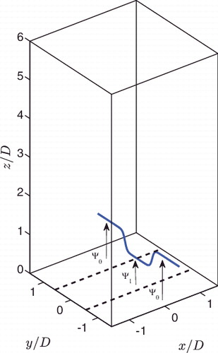
Boundary conditions in the simulations include periodic boundary conditions for the velocity, pressure and the progress variable c in the x-direction. The mean pressure gradient along the streamwise z-direction is assumed constant, and Neumann boundary conditions are imposed for the pressure at the outflow plane in the z-direction. This also holds at the outflow plane for the three velocity components, u_i, and for the combustion control variable c. Hence, (7) (8) (9)

In the y-direction pressure was held constant and equal to the atmospheric pressure, while Neumann boundary conditions are imposed for the velocity components u_i and the scalar variable c: (10) (11)

At the inflow plane, a hyperbolic tangent profile along the streamwise z-direction, W_inflow, is imposed for the inflow velocity using the following window function, Ξ: (12a) (12b) where and in (12b(12b) ). The Reynolds number of the centreline stream Re = U₁D/ν is equal to 493. For the reaction progress variable, the inflow hyperbolic profiles, W_c, are prescribed as follows: (13a) where for (12b(12b) )–(13a(13a) ) the same profiles thickness, θ, is considered. Here, the parameter θ is imposed to have the same value as the flame thickness of the premixed flamelet, l_f, to be defined later.

To ignite the cold jet mixture, a faster co-flow jet consisting of fully burned hot gases with velocity U₀ = 7 m/s and temperature T = 2240 K surrounds the low-speed stream, U₁, at the inflow plane. For a mixture, at equivalence ratio Φ = 1.0 and temperature T = 298 K, the flame front thickness, estimated from the 1D FGM database, will be l_f ≈ 0.53 mm, where l_f is computed based on the maximum gradient of the progress variable. In general, this indicates that for the reference spatial resolution five points are available to resolve the flame front. Naturally, at this level of spatial resolution one cannot resolve the thin reaction zone [12,17], δ_R. In this paper we are not simulating premixed combustion using detailed chemistry, but we use a parameterised chemistry model, i.e. FGM, where the region of the largest gradient in c represents the flame front location. The flame is parameterised with c, which by itself is well resolved on the grid, indicating that also the corresponding representation of the flame front is included well into the computational model.

At the inflow plane, turbulence is generated using random filtered fluctuations according to the method proposed in [19]. For sake of clarity, in this paper we provide a concise description of the algorithm. In this approach, turbulent fluctuations are generated for the three velocity components at each time-step from a uniform stochastic field with random numbers varying between −1 and 1. Subsequently, the generated random field is filtered in each direction using a top-hat filter of width Δ = 0.65D, such that the largest scales have a similar size compared to the width D of the cold low-speed stream region. Here, each of filtered components, , temporally drive the actually imposed fluctuations, , in terms of the following equation [19]: (14)

where the time-step δt is set to 2.10⁻⁷s, following the cases discussed in [14]. At the end of this procedure, the imposed fluctuations, , are multiplied with 4000 to obtain a turbulent intensity level I=16% of U₁. For all cases described, the turbulent fluctuations are imposed only for the three velocity components, such that, no small-scale perturbations are added to the progress variable inflow profiles.

2.2. Reference Bunsen flame

The unmodulated reference flame corresponds to the case where only turbulence is added at the inflow, i.e. without additional large-scale perturbation. This is the reference case with which all other cases will be compared. Another possible point of comparison based on a laminar flame, agitated by the applied large-scale modulation only would allow to separately discriminate the effects of the large-scale fluctuations interacting with the flame front. This would mimic a situation of a laminar Bunsen flame forced by an inflow wave reminiscent of thermo-acoustics [21,22]. In this paper we are interested in the combined effects of a large-scale spatial forcing and filtered random perturbations on the flame front and will not incorporate the laminar modulated case.

As an example of the spatial development associated with the small-scale filtered fluctuations, Figure 4 shows for the reference case, the spanwise autocorrelation R_xx of the streamwise fluctuations, w(x, t), obtained at different downstream locations.

Figure 4. Spanwise autocorrelation functions of the streamwise fluctuations, R_xx, versus the spatial separation in the x-direction. The autocorrelation functions were obtained from a snapshot of the DNS field, collected after 25 flow through-times, and computed over the x-direction at constant y and z. Lines correspond to the results of R_xx obtained at y = 0.5D and z = z₀, with z₀ = 0.5D (dashed-dotted line), z₀ = D (dashed line) and z₀ = 1.5D (solid line). D represents the width of the inflow region, D=2.4 mm, associated with the cold low-speed stream.

From the fall-off of R_xx, as shown in Figure 4, we observe that at the domain boundary in the x-direction, i.e. x = L, the autocorrelation is approximately R_xx ≈ 0, which indicates that the effect of periodic conditions is not substantial for this case [23]. In fact, the latter condition is desirable in order to obtain a more realistic flame [19]. Following a similar procedure, the longitudinal autocorrelation for the streamwise fluctuations, R_zz, was also obtained. Based on R_zz, the size of the integral scales of the flow, ℓ, is estimated using ℓ =∫^2L₀R_zzdz, for a centreline along the low-speed jet. For the unmodulated case, we obtain ℓ ≈ 0.38D. For comparison, the estimated size of the Kolmogorov scale of the unburnt jet is η ≈0.17 mm, which indicates that η is smaller than the thickness of the flame preheated zone, l_f.

From this set of parameters, we conclude that the baseline flow is characterised by a relatively low Taylor-Reynolds number Re_λ ≈ 17, defined in terms of the turbulent fluctuations generated at the inflow plane. At this Re_λ an extensive parameter study based on DNS can be performed to quantify the response of the flame to the upstream inflow modulation. Additionally, as will be shown, in all simulations in this paper the laminar flamelet structure is retained. This implies that the flame is in the wrinkled flamelet regime, which justifies the flamelet assumption for the premixed flame. In these simulations, the level of turbulent intensity imposed in the unburned gases is comparable to the laminar flame propagation speed, S⁰_L. Thus, we expect that the imposed fluctuations will not induce significant distortions in the surface of the flame beyond the wrinkled flamelet regime [8,12,24].

3. Spatially periodic large-scale forcing

Next to this random perturbation we introduce large-scale agitation for the cases where the flame is modulated. The motivation for applying such inflow agitation is to mimic the modulation of the turbulent flow as it occurs in pipe flow experiments where a compact active grid was used to stir the main flow [4], or similarly as in case of DNS of modulation of homogenous isotropic turbulence (HIT) [6]. In this paper, we follow an analogous idea in terms of the agitation of the turbulent Bunsen flame. Following the procedure discussed in [14,25], the premixed flame is spatially modulated by a set of coherent vortical structures imposed at the inflow plane, which are largely responsible for the effects of a spatial deflection acting on the jet flow.

These flow structures are confined to the region of size L × D where the cold unburned mixture is introduced. This large-scale flow, defined as a Beltrami flow type [26], is given as follows (15a) (15b) (15c)

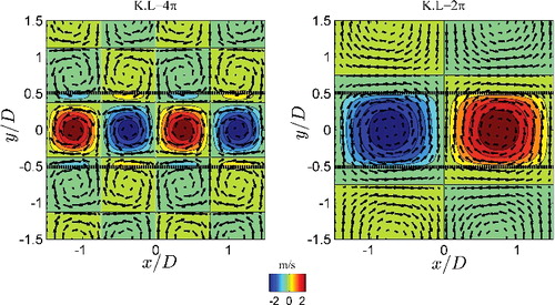
The wave-numbers, K, are based on the relation KL = 2πm in order to preserve the correct periodicity in the x direction. The integer m represents the mode that is imposed. As an example, Figure 5 shows contours of the component w_B for two different cases. If m = 2, four large-scale vortices with opposite vorticity are imposed. Another case corresponds to two vortices, m = 1, with alternating vorticity. The modulation is confined to the inflow region of size L × D by multiplying the corresponding Beltrami velocity with the window function of (12a(12a) ). Therefore, outside this region the amplitude of the structured forcing is negligible and significant coherent structures are imposed only inside the region of the low-speed stream, U₁. As an example, Figure 5 shows contours of the streamwise velocity component w_B for two set of modulation length-scales.

Figure 5. Top view of the inflow plane showing 2D contours and vectors of the streamwise velocity component, w_B, of the upstream modulation imposed at the inflow. The associated large-scale periodic flow is focused in the region of size L × D in the x- and y-direction. (left) the imposed pattern at K = 4π/L and (right) at K = 2π/L, respectively. The dashed lines represent the edges of the inflow plane region to which these coherent structures are concentrated.

The large-scale forcing amplitude is set to γ = 1.5 m/s, which is high relative to the imposed turbulent fluctuations. This yields pronounced modulation effects in the flow. In case turbulent velocity fluctuations are much larger than the large-scale modulation, the intensification effects due to the modulation tend to be reduced by the turbulence and the flame [14,25,27].

This paper focuses on the global response of the flame due to the presence of the modulation (15a(15a) –15c(15c) ) acting on the incoming turbulent co-flow jet. Here, as we mentioned the analysis of acoustical perturbations on the flame front, for instance, will not be considered. Rather, our interest is in the consequences of a complex ‘deflection pattern’ upstream of the flame, whereby mixing and turbulence intensity can be specifically enhanced.

In the next section, we describe the methods used to evaluate flame key response properties, after which the sensitivity of these properties to the spatial resolution will be assessed.

4. Global response properties

In this paper, the response of the flame to the imposed upstream modulation is characterised in terms of properties more relevant to indicate combustion intensification, such as the global flame surface wrinkling, ⟨W⟩ and the averaged flame height ⟨H⟩. As already mentioned, the former quantity provides a direct indication of the increase of the combustion rate, while the latter gives a quantitative indication of the mixture consumption efficiency.

In terms of flame surface geometric properties, i.e. the surface wrinkling W, a specialised integration procedure, over the flame front, is adopted. Initially, as in [28] we define the flame front as the progress variable iso-surface where the maximum heat release rate occurs. For the present mixture, i.e. at equivalence ratio Φ = 1.0 and standard pressure-temperature conditions, the corresponding value of the progress variable where the chemistry source is the highest occurs at c^* = 0.56. Based on this definition, we apply the quadrature approach [29] to compute the surface integral over an arbitrary volume enclosing the iso-surface of the progress variable at value c^*. Through this procedure, an accurate evaluation of geometric flame properties, e.g. surface area, total curvature, and global wrinkling, can be obtained. The integral of a density function f over an instantaneous flame front surface is obtained using the following relation [29]: (16)

where the surface S(c^*, t) corresponds to the surface associated with the iso-scalar level function F(x, y, z, t) = c^*, over which we integrate. The volume V is an arbitrary volume, in this study taken equal to the computational domain, enclosing the flame surface, S(c^*, t) [29]. In case f(x, y, z, t) ≡ 1 in (16(16) ), the total surface area of the Bunsen flame, A_f, is computed. In case f(x, y, z, t) ≡ |∇.n| the instantaneous total surface wrinkling, W(t), is determined [29]. The unitary vector, , is defined as the vector normal to the progress variable surface.

To obtain the time-averaged surface wrinkling, ⟨W⟩, firstly the instantaneous total surface wrinkling W(t) is computed with the quadrature approach for each stored sample of the 3D progress variable field. Here, each field represents independent samples of the flame. The total number of stored samples is N_s = 15, which was found to be adequate for a fair approximation of the average. To determine the average of the property extracted, we use the following relation: (17)

where W(t_i) defines the total flame wrinkling obtained for the stored 3D progress variable field at t = t_i.

For the evaluation of the time-averaged flame height, ⟨H⟩, initially we average snapshots of the 3D progress variable scalar field, c, over N_s samples: (18)

where c(x, y, z, t_i) defines an instantaneous sample of the 3D progress variable scalar field at time instant t = t_i. From the time averaged scalar c field, ⟨c(x, y, z)⟩, we extract the iso-contours at c^*. Subsequently, the height of the flame taken at all yz-planes is spatially averaged over the periodic x direction, leading to the averaged flame height ⟨H⟩. In this procedure, the flame height is the maximum value of the z-coordinate as obtained from the spatially averaged yz-planes of ⟨c^*(x, y, z)⟩.

The results presented in this paper show direct analogies with others studies in modulated turbulence [1–4]. We also consider the effects of the applied modulation in the average dissipation rate, ⟨ϵ⟩ and in the average enstrophy, ⟨Ω⟩. Both quantities provide a direct indication of the dynamical effects of the inflow modulation on the micro-mixing. Here, to evaluate ⟨ϵ⟩ for the variable-density flow investigated we included the density variation in the computation of the dissipation rate over the whole domain using: (19) where μ(T) is the temperature-dependent dynamic viscosity and S_ij the rate-of-strain tensor. We evaluate (19(19) ) using stored snapshots of the entire flow field, extracted at the instant t_i. Subsequently, we average the stored fields over the number of samples, N_s, using a similar procedure as described in (18(18) ).

The flow response to the imposed modulation is quantified in terms of the global average dissipation rate, ⟨ϵ⟩_xyz, and the total enstrophy, ⟨Ω⟩_xyz. Here, both quantities are defined based on their corresponding integral over the whole domain volume: (20a) (20b) where the averaging volume V is taken equal to L × L × 4L, with L = 1.5D. The time-averaged vorticity magnitude, ⟨|∇ × u|⟩, is computed following the averaging procedure given by (18(18) ).

Next we consider the sensitivity of flame solutions to different grid resolutions. This analysis will be based on a grid refinement approach for the unmodulated reference Bunsen flame.

4.1. Grid refinement analysis

In this section, the dependence of some characteristic quantities on the spatial resolution is evaluated for the unmodulated reference case. We check changes in the time-averaged contours associated with the flame front and in the mean magnitude of the progress variable gradient, ⟨|∇c|⟩, with respect to the resolution considered. Both quantities are relevant for the cases where a large-scale modulation will be imposed to agitate the flame. While the averaged contours of the progress variable are used to determine the averaged flame height response ⟨H⟩, the mean magnitude of the progress variable gradient, ⟨|∇c|⟩, quantifies the effects of turbulence into the flame inner structure [28].

To determine the mean gradient, ⟨|∇c|⟩, we first determine |∇c| for a number of snapshots over the whole domain using a central difference second-order scheme, after which results of |∇c| are conditionally averaged based on the local value of the progress variable and stored using 50 bins distributed between 0 and 1. At these number of bins, the computed gradient, ⟨|∇c|⟩, shows to be statistically converged and quite similar to those observed for premixed flames [28].

Grid refinement results for the unmodulated flame are shown in Figure 6. Results for the time-averaged progress variable contours at c^* illustrate the sensitivity of the solution to different resolutions. A clear convergence trend is established as the grid resolution increases. For the contours analysed, convergence is sufficiently achieved on the grid 64 × 64 × 128 in comparison to the finest resolution at 128 × 128 × 256 since the progress variable contours of c^* are almost on top of each other. In case of ⟨|∇c|⟩, results show that despite the different resolutions similar trends are observed in all cases. As can be seen, a consistent grid convergence occurs as the resolution increases, such that, at the resolution 64 × 64 × 128 no significant differences in the analysed quantity occurs when compared to the finest resolved case.

Figure 6. Unmodulated flame results: (a) Averaged flame front contours for the scalar c^* and (b) Mean magnitude of the progress variable gradient ⟨|∇c|⟩, at different resolutions. Lines correspond to the following grids: 32 × 32 × 64 (dashed line), 64 × 64 × 128 (dashed-dotted line), and 128 × 128 × 256 (solid line).

Based on these results, a good degree of grid independence is apparent at the mid-level refinement. Thus, we select the resolution 64 × 64 × 128 in the sequel to investigate the cases where a large-scale modulation is used to agitate the baseline Bunsen flame. Some general features of the large-scale agitation are introduced next.

5. Modulated Bunsen flame

The effects of the large-scale modulation are first characterised in terms of global properties of the flow, e.g. ⟨ϵ⟩_xyz and ⟨Ω⟩_xyz. Interestingly, when the volume-averaged dissipation rate ⟨ϵ⟩_xyz is determined as shown in Figure 7, a definite effect shows up when the large-scale perturbation consists of structures of sizes from K = 8π/L to K = 2π/L. For comparison purposes, the results are normalised by the values obtained for the unmodulated reference flame. Clearly, both properties show a maximum at relatively low wave-numbers in this case. This suggests that the imposed modulation can actually stimulate an enhanced effect in these properties, at least globally, also in the reactive flow. It should be noted that the enhancement shown in Figure 7 is due to a large response effect found at locations near the inflow plane, since further downstream the modulation effects tends to decay very rapidly due to combustion. This explains the fact that the flow response at high wave-numbers is not small compared to the maximum observed in both properties for lower modes, which indicates that although restrict to regions near the inflow plane the modulation contribution at such locations are capable of sustain a larger effect in the volume-averaged quantities than the unmodulated case.

Figure 7. (a) Total enstrophy ⟨Ω⟩_xyz and (b) global averaged dissipation rate, ⟨ϵ⟩_xyz, as a function of the spatial mode, KL/π. In this figure, both properties are normalised by the value of the reference unmodulated case, i.e. ⟨Ω₀⟩_xyz and ⟨ϵ₀⟩_xyz.

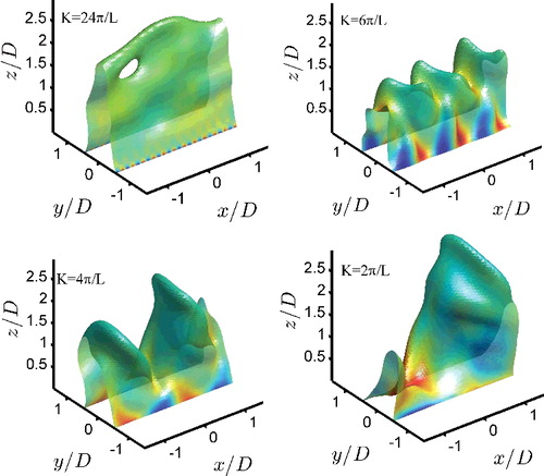
For a qualitative impression of the flame response to different modulation length-scales, initially we present in Figure 8 the 3D snapshots of the flame front at different modulation wave-numbers K. Significant qualitative changes in the flame surface are apparent as the modulation wave-number is altered. The flame distortion is the strongest at modulation wave-number K = 6π/L. The imposed set of small length-scales at high K does not appear to result in large flame folding and the modulation effect very rapidly decays downstream. Conversely, considerable changes in the flame structure are induced throughout the domain in case K is sufficiently small.

Figure 8. 3D snapshots of the flame front after 5 flow-through times coloured with vorticity in the z-direction, . Results for modulation wave-numbers from top left to bottom right: K = 24π/L, K = 6π/L, K = 4π/L, and K = 2π/L. The flame front corresponds to the surface of maximum heat release rate, i.e., c^* = 0.56.

The effects due to turbulence combined with the imposed large-scale modulation on the mean structure of the flame front are shown in Figure 9, where we compute the conditioned pdf of the magnitude of the progress variable gradient for all modulated cases. For comparison, the magnitude of the progress variable gradient obtained for the one-dimensional laminar flame, with CHEM1D, is also included. As a measure of variability of the scalar gradient within the flame, the variance of the mean gradient is also determined. As can be observed, results in Figure 9 show that the mean flame structure is not strongly affected by turbulence or the applied modulation, and that at regions where c ≲ 0.7, large variances are observed for the cases K = 6π/L and K = 2π/L when compared with the unmodulated flame or cases with high modulation wave-number, in this case K = 24π/L. Combined with these results, the small level of turbulent fluctuations in these simulations indicates that the premixed flame is in the wrinkled flamelet regime [12,17].

Figure 9. (Top) Results of the conditioned pdf of the magnitude of the scaled progress variable gradient versus the progress variable. The mean scalar gradient obtained for the one-dimensional premixed flamelet is also shown (solid line with ○ symbols), (bottom) variance of the mean scalar gradient, ⟨|∇c|²⟩ − ⟨|∇c|⟩², as a function of c. In both figures, lines correspond to the following cases: unmodulated (dashed-dotted line), K = 24π/L (dotted line), 6π/L (dashed line), and 2π/L (solid line).

In addition, the results in Figure 9 suggest that the increased local dilatation and penetration of small scales of the flow into the flame region might occur more intensely for cases modulated at low K, although the average effect is rather small relative to the unmodulated flame. It is quite suggestive that the large variations in ⟨|∇c|⟩ occur for modulation at K = 6π/L, since this result qualitatively correlates with the observed distortions in the flame front shown in Figure 8, for a modulation set at such wave-number. For all cases, at hotter flame regions, e.g. c > 0.7, the effects of turbulence and the applied modulation are negligible. This is indicated by the decreasing variance as the progress variable increases.

Next we quantify the modulation effects on the turbulent Bunsen flame in terms of the flame wrinkling and the flame height. As already mentioned, we consider the global surface wrinkling ⟨W⟩ and the averaged flame height ⟨H⟩ to characterise the flame response since such properties are suitable quantities to express the effect of external modulation on the flame intensification. In Figure 10, results of both properties are shown. Results of ⟨H⟩ show the susceptibility of the time-averaged flame height to the imposed large-scale agitation. As can be seen, a maximum response occurs for both properties when the modulation scale is set to scales in the range K = 4π/L to K = 8π/L. The largest enhancement of ⟨W⟩ at K = 6π/L is in qualitative agreement with the significant flame distortions observed in the flame snapshots shown in Figure 8.

Figure 10. (Top) Results of the averaged global surface wrinkling ⟨W⟩ and (bottom) the averaged flame height ⟨H⟩ as a function of the modulation mode KL/π. The results of ⟨W⟩ are normalised by the global wrinkling obtained for the unmodulated reference case, W₀, while the response quantity ⟨H⟩ is normalised by the width D.

From the resonance effect of the flame properties shown in Figure 10, a connection with the enhancement of turbulence by the imposed perturbation can be established. As discussed in [14], for the co-flow planar jet, the enhancement of turbulent properties, e.g. scalar dissipation rate ϵ, is strong when the inflow modulation scale is of the same order as the jet integral scale [25,27]. Such scales in the flow lead to an increase of the surface area of the flame due to an increase of the global surface wrinkling ⟨W⟩. An increased flame intensity reduces the mean flame height ⟨H⟩ since a more wrinkled front will correspond to an increase in the turbulent burning velocity. This property quantifies directly the increase in the consumption rate of the unburned reactants by the premixed flame.

6. Conclusions

The effects of a spatially periodic modulation acting on a turbulent Bunsen flame were investigated using direct numerical simulations of the Navier-Stokes equations coupled with a tabulated chemistry technique, i.e. the FGM. The stoichiometric premixed Bunsen flame was agitated in space and time by a hybrid perturbation consisting of filtered small-scale random perturbations and a coherent large-scale spatially periodic modulation of specific wave-number K. For properties related with the unburned mixture, an enhancement of approximately 45% in the volume-averaged dissipation rate ⟨ϵ⟩ and of about 25% in the averaged enstrophy ⟨Ω⟩, in comparison with the unmodulated case, was obtained when the agitation consisted of length-scales with size related to the inflow characteristic length-scale D. For the inflow modulation, such scales are in general associated with wave-numbers ranging from K = 4π/L to K = 8π/L.

The flame response was characterised in terms of the average flame height, ⟨H⟩ and the averaged flame surface wrinkling ⟨W⟩. Both flame quantities respond quite sensitively and show definite effects to the large-scale modulation. For example, in terms of ⟨W⟩, a significant enhancement in the surface wrinkling occurs for a modulation based on wave-numbers from K = 4π/L to K = 8π/L, while for ⟨H⟩ a shorter flame is stimulated preferably with modulation K = 4π/L. In the latter case, the development of a large wrinkled surface generates a flame front with an average height almost 30% shorter than the unmodulated flame. The presence of a maximum flame response at such modulation wave-number K suggests that the enhancement in the small-scale mixing, e.g. represented by the dissipation rate leads to a substantial effect in the flame responsiveness. At the agitation scales where the maximum response is observed, the average flame height, ⟨H⟩, takes a clearly defined minimal value while the surface wrinkling, ⟨W⟩, presents an increase by more than a factor of 2 in comparison with the unmodulated case. These results indicate the existence of preferential scales for flame agitation and illustrate the potential application of modulated turbulence in generating appropriate conditions for more efficient fuel consumption, i.e. in more compact, premixed Bunsen flames.

In this paper, the dependence of the multiscale flame intensification on the flow's Reynolds number, Re, is not treated. It is expected that the penetration length of the modulation effects as well as the spectral composition of the flow will vary considerably with increasing Re. Additionally, the response analysis was restricted to a methane Bunsen flame, thus the possibility to enhance combustion rate through turbulence modulation involving other types of fuels, e.g. propane, hydrogen mixtures, is of much interest and currently under consideration.

Acknowledgments

The authors would like to acknowledge the Dutch Technology Foundation STW for the financial support. Computations were done at SARA, made possible by support from NWO, grant SH-061.

Disclosure statement

No potential conflict of interest was reported by the authors.

Additional information

Funding

Dutch Technology Foundation STW; NWO [grant number SH-061].

References

- Kuczaj AK, Geurts BJ. Mixing in manipulated turbulence. J Turbul. 2006;7: N67.
- Cekli HE, Tipton C, van de Water W. Resonant enhancement of turbulent energy dissipation. Phys Rev Lett. 2010;105(4):044503.
- Cadot O, Titon JH, Bonn D. Experimental observation of resonances in modulated turbulence. J Fluid Mech. 2003;485: 161–170.
- Verbeek A, Pos R, Stoffels G, et al. A compact active grid for stirring pipe flow. Exp Fluids 2013;54(10):1–16.
- Verbeek AA, Bouten TW, Stoffels GG, et al. Fractal turbulence enhancing low-swirl combustion. Combust Flame 2015;162(1):129–143.
- Kuczaj AK, Geurts BJ, Lohse D. Response maxima in time-modulated turbulence: direct numerical simulations. EPL (Europhys. Lett.) 2006;73(6):851.
- Landau L. On the theory of slow combustion. Acta Physicochim. URSS 1944;19(1):77–85.
- Law CK. Combustion physics. New York (NY): Cambridge University Press; 2006.
- Creta F, Fogla N, Matalon M. Turbulent propagation of premixed flames in the presence of Darrieus–Landau instability. Combust. Theory Model. 2011;15(2):267–298.
- Paul RN, Bray KNC. Study of premixed turbulent combustion including Landau–Darrieus instability effects. In: 26th Symposium (international) on combustion. Pittsburgh (PA): The Combustion Institute; 1996. p. 259–266.
- Matalon M. Intrinsic flame instabilities in premixed and nonpremixed combustion. Annu Rev Fluid Mech. 2007;39: 163–191.
- Peters N. Turbulent combustion. Cambridge: Cambridge University Press; 2000.
- Van Oijen J, Bastiaans R, Groot G, et al. Direct numerical simulations of premixed turbulent flames with reduced chemistry: validation and flamelet analysis. Flow, Turbul Combust. 2005;75(1-4):67–84.
- de Souza TC, Geurts B, Bastiaans R, et al. Steady large-scale modulation of a moderately turbulent co-flow jet. J Turbul. 2014;15(5):273–292.
- CHEMID, A one-dimensional laminar flame code. Eindhoven University of Technology. Available from: https://www.tue.nl/en/university/departments/mechanical-engineering/research/research-groups/multiphase-and-reactive-flows/our-expertise/research- topics/chem1d/.
- Smith G, Golden D, Frenklach M, et al. GRImech 3.0 reaction mechanism. Berkeley; 2000.
- Griffiths JF, Barnard JA. Flame and combustion. London: Chapman and Hall; 1995.
- van Oijen JA. Flamelet-generated manifolds: development and application to premixed laminar flames. Eindhoven: Technische Universiteit Eindhoven; 2002.
- Vreman A, Bastiaans R, Geurts B. A similarity subgrid model for premixed turbulent combustion. Flow, Turbul Combust 2009;82(2):233–248.
- Trottenberg U, Oosterlee CW, Schuller A. Multigrid. New York (NY): Academic Press; 2001.
- Candel S. Combustion instabilities coupled by pressure waves and their active control. In: 24th Symposium (international) on combustion. Pittsburgh: The Combustion Institute; 1992. p. 1277–1296.
- Lieuwen T. Modeling premixed combustion-acoustic wave interactions: a review. J Propulsion Power 2003;19(5):765–781.
- Pope SB. Turbulent flows. Cambridge: Cambridge University Press; 2000.
- Poinsot T, Veynante D. Theoretical and numerical combustion. Philadelphia: Edwards; 2005.
- de Souza TC. Modulated turbulence for premixed flames. Eindhoven: Technische Universiteit Eindhoven; 2014.
- Majda AJ, Bertozzi AL. Vorticity and incompressible flow. Cambridge: Cambridge University Press; 2002.
- Tyliszczak A, Geurts BJ. Parametric analysis of excited round jets-numerical study. Flow, Turbulence Combust 2014;93(2):221–247.
- Moureau V, Domingo P, Vervisch L. From large-eddy simulation to direct numerical simulation of a lean premixed swirl flame: filtered laminar flame-pdf modeling. Combust Flame 2011;158(7):1340–1357.
- Geurts BJ. Mixing efficiency in turbulent shear layers. J. Turbul. 2001;2(17):1–23.