Analysis of structure function equations up to the seventh order

ABSTRACT

We examine balances of structure function equations up to the seventh order N = 7 for longitudinal, mixed and transverse components. Similarly, we examine the traces of the structure function equations, which are of interest because they contain invariant scaling parameters. The trace equations are found to be qualitatively similar to the individual component's equations. In the even-order equations, the source terms proportional to the correlation between velocity increments and the pseudo-dissipation tensor are significant, while for odd N, source terms proportional to the correlation of velocity increments and pressure gradients are dominant. Regarding the component equations, one finds under the inertial range assumptions as many equations as unknown structure functions for even N, i.e. can solve for them as function of the source terms. On the other hand, there are more structure functions than equations for odd N under the inertial range assumptions. Similarly, there are not enough linearly independent equations in the viscous range r → 0 for orders N > 3.

KEYWORDS:

• Structure function equations
• structure function trace equations
• isotropic turbulence

1. Introduction

One of the several different approaches to analyse the multi-scale behaviour of turbulent flows is to examine the statistical properties of velocity differences, as introduced and pioneered by Kolmogorov [1,2] (hereafter referred to as K41). Assuming isotropy, the moments of the velocity difference Δu_i = u_i(x_j + r_j) − u_i(x_j), i.e. the structure functions D_m,n = ⟨(Δu₁)^m(Δu₂)ⁿ⟩ depend only on the magnitude of the separation vector r_i, but not its orientation. Kolmogorov [2] derived from the Kármán-Howarth equation a transport equation for the second-order structure function ∂D_{2, 0}/∂t. He then assumed decaying isotropic turbulence to replace the decay of kinetic energy k with the dissipation ϵ = 2νs_ijs_ij, ∂ ⟨k⟩/∂t = − ⟨ϵ⟩, where s_ij = (∂u_i/∂x_j + ∂u_j/∂x_i)/2. After neglecting the unsteady term ∂D_{2, 0}/∂t, he obtained (1) cf. e.g. the discussion and derivation in Monin and Yaglom [3] or Rotta [4]. This allowed him to solve Equation (1(1) ) for the third-order structure function D_{3, 0} in the inertial range, where viscous effects can be neglected as well as for D_{2, 0} in the viscous range r → 0, where the transport term on the l.h.s. can be neglected. With these findings, Kolmogorov [1] postulated two similarity hypotheses, namely that structure function statistics should be determined by ⟨ϵ⟩ in the inertial range and by ⟨ϵ⟩ and ν in the viscous range and introduced dissipative scales valid for the second order, the Kolmogorov scale η = (ν³/⟨ϵ⟩)^1/4 and velocity u_η = (ν⟨ϵ⟩)^1/4.

Structure function equations of arbitrary order can be derived from the Navier–Stoke equations, cf. Yakhot [5] and Hill [6]. While Yakhot's derivation is based on a moment generating function, Hill derived a transport equation for the velocity difference Δu_i, which can be used as building block for higher order equations for ⟨Δu_iΔu_j…⟩. The equations of Hill were derived without additional assumptions besides continuity and are therefore valid for any incompressible flow, but can be further simplified under the constraints of (local) homogeneity and (local) isotropy. Then, the structure function equations are determined by two different source terms, the first stemming from correlations of velocity increments and the pressure gradient, ⟨Δu_iΔu_j…(∂p/∂x_k − ∂p′/∂x′_k)⟩ (henceforth called pressure source terms), the second one from correlations of velocity increments and the pseudo-dissipation tensor, ⟨Δu_iΔu_j…(ε_kl + ε′_kl) (hereafter called dissipation source terms). Here, ε_ij is the pseudo-dissipation tensor at point x_i = x′_i + r_i and ε′_ij at x′_i, (2) The transport equations for the second-order structure functions D_{2, 0} and D_0,2 were examined by Hill [7] in detail. Assuming local homogeneity (but not isotropy), Hill obtained (3) with (4) where p is the pressure. In contrast to Equation (1(1) ) derived by Kolmogorov, Hill's more general Equation (3(3) ) contains averages of components of the pseudo-dissipation tensor ⟨ε_ij⟩ instead of the mean of the dissipation ⟨ϵ⟩. The two equations can be reconciled by noting that due to local homogeneity, ⟨ε_ij⟩ = ⟨ε′_ij⟩ and due to local isotropy, ⟨ε₁₁⟩ = ⟨ε₂₂⟩ = ⟨ε⟩/3 where (5) is the pseudo-dissipation. Here and in the following, repeated indices imply summation so that ε_ii is a trace. Moreover, due to local isotropy, local homogeneity and continuity, ⟨ε⟩ = ⟨ϵ⟩ and τ_ij = 0, so that Equations (1(1) ) and  (3(3) ) are analogous under these assumptions.

The transport equations for the third-order structure functions D_{3, 0} and D_{1, 2} (i.e. equations for ∂D_{3, 0}/∂t and ∂D_{1, 2}/∂t) were analysed by Hill and Boratav [8] under the assumption of homogeneity and isotropy. They found that the transport terms in these equations are balanced by the components of the tensor ⟨Δu_iΔu_j(∂p/∂x_k − ∂p′/∂x′_k)⟩, i.e. the third-order pressure source terms, while the dissipation source terms are negligible. Kurien and Sreenvasan [9] examined higher order structure function equations and measured scaling exponents of the structure functions. These measurements are in good agreement with exponents resulting from a mean-field theory presented by Yakhot [5] to close the structure function equations. Nakano et al. [10] examined the source terms of the longitudinal structure function equations in detail. They found that the normalised longitudinal dissipation source terms approached an asymptotic, presumably constant value in the inertial range for higher orders. Gotoh and Nakano [11] analysed longitudinal and mixed odd-order structure function equations using direct numerical simulation (DNS). Similar to the findings of Hill and Boratav [8], they concluded that the terms ⟨Δu_iΔu_j…(∂p/∂x_k − ∂p′/∂x′_k)⟩ are important for the longitudinal balances but may be neglected for the mixed balances. Neglecting both the dissipation source terms as well as the pressure source terms in the odd-order equations allowed Grauer et al. [12] to interpret the remaining relations between the even-order structure functions as Taylor series, which they used to rescale the even-order structure functions. They then found that the rescaled longitudinal and mixed structure functions D_{N, 0} and D_{N − 2, 2} (nearly) collapse. Gotoh and Nakano [11] furthermore presented a closure for the pressure source terms. Their model was further refined by Yakhot [13].

The fourth-order structure function equations for D_{4, 0}, D_{2, 2} and D_{0, 4} were examined by Peters et al. [14] as well as the trace D_[4] = D_4,0 + 4D_2,2 + 8D_0,4/3. Deriving a transport equation for the dominant source terms in these equations, which are components of the tensor ⟨Δu_iΔu_j(ε_kl + ε′_kl)⟩ (i.e. the fourth-order dissipation source terms), Peters et al. found terms proportional to the second moment of the pseudo-dissipation ⟨ε²⟩, in direct contradiction of Kolmogorov's [1] original similarity hypotheses that structure function statistics should depend on the mean ⟨ϵ⟩. Indeed, the K41 similarity hypotheses were questioned by Landau (cf. the discussion in Frisch [15]) shortly after their publication.

Since the structure function equations are exact, the structure functions can be obtained by solving the system. However, the system is unclosed and additional assumptions are required. In a first step, we examine the balances of the equations and the source terms up to the seventh order. Some of these balances were already analysed and discussed in the literature, but not all of them. Particularly, the trace equations from which one can determine the structure function trace as detailed below have never been examined to our knowledge. While we do not try to close the source terms, we hope that the balances are of use for future work. We have numerically calculated all terms found in the system of structure function equations as derived by Hill [6] under the assumption of homogeneity and isotropy using direct numerical simulations of isotropic turbulence with Reynolds number up to Re_λ = 754. The characteristics of the DNS can be found in the Appendix.

In the following, we discuss the system of structure function equations in Section 2. We then look at the balances of the structure function equations up to the seventh order in Section 3 and proceed to analyse the trace of the equations in Section 4, before concluding our findings in Section 5.

2. System of equations

Let us briefly discuss the system of structure function equations as derived by Hill [6]. Following Hill, these equations are derived by subtracting the Navier–Stokes equations at point x′_i from the ones at x_i, where x_i = x′_i + r_i, i.e. r_i is the separation vector aligned for convenience without loss of generality with the x₁ −axis. After a coordinate transform (x_i, x′_i) → (X_i, r_i) (where X_i = (x_i + x′_i)/2), averaging, neglecting terms with derivatives with respect to X_i due to local homogeneity and using local isotropy to rewrite the gradient and Laplacian in terms of r = |r_i|, one obtains equations for the structure functions D_{m, n} = ⟨Δu^m₁Δuⁿ₂⟩, where Δu_i = u_i − u′_i. Here, we use N = n + m to denote the order and m and n denote the exponents of longitudinal and transverse velocity increments, respectively. This is not to be confused with explicit notation such as A_ij = ..., where i and j can be any index. In general, u_i = u_i(x_i, t) and u′_i = u_i(x′_i, t′), i.e. the two-points are separated in time by t − t′ as well as in space by r_i and the more general change of coordinates is with Δt = t − t′ and , see Hill [16]. Assuming local stationarity as well as local homogeneity, the two-point statistics then depend on r_i and Δt, but not X_i and . In the following, we take t = t′, i.e. have the two points separated only in space. Then, we have (6) where possible additional terms stemming from some large-scale forcing have been neglected. All orders have the same general structure. In the Nth-order structure function equation, there are convective terms containing structure functions of order N + 1 () on the l.h.s. and on the r.h.s. pressure source terms , dissipation source terms and viscous terms , all of order N. The source terms are (7) where ε_ij is the pseudo-dissipation tensor defined by Equation (2(2) ) and curly braces denote the sum of all terms of a given type that produce symmetry under interchange of indices. For instance at the fourth order (8) or at the third order (9) and thus, e.g. (10) where E_3,0 = E₁₁₁,E_2,2 = E₁₁₂₂,T_1,2 = T₁₂₂ and T_0,4 = T₂₂₂₂.

Note that at the second order, the dissipation source terms E_{2, 0} = 2 < ε₁₁ + ε′₁₁ > =4 < ε₁₁ > and E_{0, 2} = 2 < ε₂₂ + ε′₂₂ > =4 < ε₂₂ > are independent of r under the assumption of local homogeneity. Also, the pressure source terms vanish due to local isotropy, cf. e.g. Hill [17]. Since the second-order source terms ⟨ ε₁₁ ⟩ = ⟨ε₂₂⟩ = ⟨ε⟩ /3 are then independent of r under the assumption of homogeneity, ⟨ε⟩ can be interpreted as an external parameter. This breaks down at any higher order N > 2, since the and then depend on r and the do not vanish. If one derives consecutive transport equations for higher order dissipation source terms, one finds for even N the higher moments of the pseudo-dissipation, cf. Peters et al. [14].

It should be stressed that one finds the pseudo-dissipation ⟨ε⟩ in the system of structure function equations and not the dissipation ⟨ϵ⟩ for N = 2 and similarly for the higher orders, where again not the moments of the dissipation ϵ but the moments of the pseudo-dissipation ε are found when one derives consecutive transport equations for the dissipation source terms as outlined by Peters et al. [14]. While ⟨ε⟩ = ⟨ϵ⟩ under the assumption of local homogeneity, there are no exact analogous relations at higher orders. Consequently, Kolmogorov's [1] similarity hypothesis that structure functions should depend on the mean dissipation ⟨ϵ⟩ (as well as the viscosity ν in the viscous range) or modifications such as replacing the mean with higher moments are at first glance not in line with the system of structure function equations derived from the Navier–Stokes equations. While there are no analytical results for the ratios ⟨ε^N⟩/⟨ϵ^N⟩ for N > 1, they were found to have the same Reynolds number scaling and differ only by an empirical constant, provided the Reynolds number is large enough. Therefore, one can replace the moments of the pseudo-dissipation ε with the moments of the dissipation ϵ for scaling purposes and phenomenology of large Reynolds number asymptotics.

Since we have aligned the separation vector r_i with the x₁-axis without loss of generality, i.e. r_i = (r, 0, 0), all isotropic two-point tensors with 3-component can be expressed equivalently by corresponding 2-components, cf.  Equation (4.4) of Hill [6]. For instance, one finds that <Δu₁(Δu₃)² > = < Δu₁(Δu₂)² > and similarly at higher orders. This implies that we do not have to consider transport equations for structure functions with 3-component, since they do not contain additional information.

The functional form of the gradient and Laplacian has been calculated by Hill [6] using a matrix algorithm and recently corrected, see https://arxiv.org/abs/physics/0102063; they are shown in Table 1 for N = 2 to N = 8 for reference.

Table 1. Isotropic form of the transport and viscous terms in the structure function equations for N = 2 to N = 8 as given by Hill [6], see https://arxiv.org/abs/physics/0102063 for the corrected version.

	Transport term	Viscous term
N = 2
N = 3
N = 4
N = 5
N = 6
N = 7
N = 8

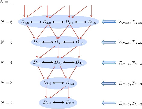
Therefore from Equation (6(6) ), there is a coupling to the next higher order structure functions via the convective terms and an inter-order coupling by the viscous terms while the and terms act as sources (or sinks, depending on their sign). This tree-like structure is visualised in Figure 1, where the coupling between different orders is indicated by the red vertical arrows (referring to the transport terms) and the inter-order coupling via the viscous terms by the black horizontal arrows. One therefore finds a system of coupled partial differential equations, where the solutions are obtained by advancing the system in time (or until the system reaches its steady state for forced turbulence) with boundary conditions as determined by the viscous range and some initial conditions for the structure functions. However, the resulting system of equations is unclosed due to the coupling to the higher order structure functions stemming from the transport term, i.e. the closure problem of turbulence. Well-known closures to overcome this issue are the quasi-normal approximation and its modifications (see Lesieur [18] and references therein for an overview), where traditionally the fourth-order structure functions are expressed in terms of the square of the second by assuming a vanishing fourth-order cumulant. Another approach is to close the system using an eddy viscosity ansatz of the form , see, e.g. Oberlack and Peters [19] or more recently Thiesset et al. [20]. The closure of Oberlack and Peters was used by Schaefer et al. [21] and Boschung et al. [22] to close the second-order equations and was found to be in very good agreement with DNS data. In any case, the source terms and (Equation (7(7) )) need to be closed and the resulting closure may introduce additional coupling between orders and structure functions. Source term closures have been developed, e.g. by Gotoh and Nakano [11] and Yakhot [5,13], but are not discussed here in the following. Note that it is possible to derive equations for the source terms, as carried out by Peters et al. [14] for the fourth-order source terms. However, these equations contain additional unclosed terms.

Figure 1. Coupling between structure function equations.

The system of equations is complemented by two equations relating the second and third-order structure functions (11) and (12) derived from the continuity equation, cf. e.g. Monin and Yaglom [3]. However, there are no analogous higher order relations. If the flow is statistically steady, the derivatives with respect to time may be neglected. For that reason, the unsteady terms are not discussed in the numerical analysis of the structure functions below in Sections 3 and  4.

2.1. Viscous range

For r → 0, the pressure source terms , while the dissipation source terms are to leading order , because ε′_ij + ε_ij → 2ε_ij for r → 0. Moreover, the transport terms and the viscous terms . Therefore, the viscous terms are balanced by the dissipation source terms in the viscous range. Consequently, one may neglect the convective terms of order N + 1 as well as the pressure source terms for small r → 0. This implies that the equations of order N are decoupled from the equations of order N + 1. In other words, in the viscous range the structure functions of order N contained in the viscous terms are completely determined by the dissipation source terms. At first glance, it would seem that there are as many equations as unknown structure functions for all orders in the viscous range if the dissipation source terms are known, cf. Figure 1 and the right column of Table 1. However, this is not the case, as not all equations are linearly independent. For instance, at the second order, there are two equations for D_2,0 and D_0,2, which are both linearly dependent, while at the fourth order, there are three equations for the three unknowns D_4,0, D_2,2 and D_0,4, again one of which can be written as sum of the other two (cf. Peters et al. [14]). Note that Equation (11(11) ) can be used to close the second-order equations in the viscous range, cf. e.g. Monin and Yaglom [3]. For N = 3, one finds the exact relations for the third-order structure functions in the viscous range: (13) which are analogous to the second-order results. A derivation based on the third-order equations can be found in the supplemental material. The third-order structure functions could also be expressed in a more familiar form in terms of the skewness of the longitudinal velocity gradient.

For higher orders, one can derive consecutive transport equations for and then look at the balance in the viscous range. For the fourth-order equations N = 4, this was carried out by Peters et al. [14]. There, the Laplacian of is balanced by a sum of squares of the pseudo-dissipation ⟨ε_ijε_kl + ⋅⋅⋅⟩. Thus, one finds that the fourth-order structure functions in the viscous range are determined by squares of the components of the pseudo-dissipation tensor and the viscosity ν only. Similar results are obtained for higher orders; e.g. the sixth-order structure functions for r → 0 are determined by ⟨ε_ijε_klε_mn +⋅⋅⋅⟩ and ν. However, the exact relations cannot be obtained, because there are not enough equations to solve the system as discussed above. Again, note that it is the moments of pseudo-dissipation ⟨ε^N⟩ rather than the moments of the dissipation ⟨ϵ^N⟩ which are found to determine the structure functions in the viscous range when one solves the structure function balance equations.

The lack of higher order equations stemming from continuity thus seems to prohibit any exact results for N > 3 in the viscous range. However, it is possible to relate the longitudinal even moments of the velocity gradient to moments of the dissipation ϵ. The procedure was outlined by Siggia [23], who derived a generating function relating all components of the strain tensor ⟨s_ijs_kl…⟩. One then finds that all longitudinal even-order structure functions of order N in the viscous range depend on the moments of the dissipation <ϵ^N/2 > and the viscosity ν, cf. Boschung [24]. However, there are no exact results for mixed or transverse structure functions as well as for any odd-order structure functions. Since the ratios ⟨ε^N⟩/⟨ϵ^N⟩ as well as the ratios of moments of the components to the moments of the dissipation are constant at sufficiently large Reynolds number, this is not at odds with the viscous range solution of the system of structure function equations described above.

Consequently, the structure functions in the viscous range can be written as (14) where C_m,n are Reynolds number independent prefactors. One can then define order-dependent scales (15) cf. Boschung et al. [25], which collapse the structure functions in the viscous range.

To conclude, the probability density function (pdf) of the dissipation ϵ in combination with the viscosity ν can therefore be thought of as boundary conditions r → 0 for the structure functions in the system of partial differential equations shown in Figure 1.

2.2. Inertial range

In the inertial range situated between the very small scales and the large integral scales L (η ≪ r ≪ L), viscosity has a negligible influence and therefore the viscous terms can be neglected. In this limit, the structure functions of order N + 1 are determined by integrating the equations of order N and are completely determined by the source terms and . Particularly, there are only enough equations to determine the structure functions for even orders, e.g. for the sixth-order equations there are four equations for four odd-order structure functions D_{7, 0}, D_{5, 2}, D_{3, 4} and D_{1, 6}. If the source terms are known, one can then proceed to successively integrate the equations starting with the equation with the most transverse components (i.e. here D_{1, 6}). On the other hand, at the fifth-order equations, there are only three equations for four structure functions D_{6, 0}, D_{4, 2}, D_{2, 4} and D_{0, 6}, and the same holds for all odd-order equations. That is, there is the peculiar situation that while it is possible to derive equations for all structure functions at arbitrary order, only odd-order structure functions can be determined in terms of and using inertial range approximations without resorting to additional closures. Again, the second order is special inasmuch as the pressure source terms vanish due to local isotropy (cf. e.g. Hill [17]) and the dissipation source terms are proportional to the pseudo-dissipation <ε > as discussed above. One can then solve the transverse second-order equation to obtain D_{1, 2} and insert the result into the longitudinal equation to calculate D_{3, 0}. This yields (16) As the integration is starting from r = 0, the contributions by the viscous terms were neglected. That is, the integral is not complete and consequently both equations hold asymptotically for large (infinite) Reynolds numbers. These results were first derived by Kolmogorov [2] from the Kármán-Howarth equation; again he had ⟨ϵ⟩ instead of ⟨ε⟩.

The results  (16(16) ) are rightfully considered to be of paramount importance, as they result from the Navier–Stokes equations and are non-trivial. Noticeably, they are also the only exact results concerning structure functions in the inertial range, because the source terms are exactly known (or, more precisely, can be treated as parameters of the flow). This is not the case for all other orders, where the pressure source terms contribute and both source terms depend on r.

If one assumes that the structure functions follow a power law in the inertial range of the form (17) then the scaling exponents ζ_m,n (as well as the prefactors C_m,n) have to be contained in the system of equations. Obviously, this is only the case if the source terms also follow a power law in the inertial range. Noticeably, the sum of two pure power laws and (with A₁, A₂ and α₁ and α₂ being constants) only results exactly in a pure power law P₃ = P₁ + P₂ if α₁ = α₂ = α₃. In other words, a scaling as Equation (17(17) ) with r-independent C_m,n and ζ_m,n would require all pressure source terms and dissipation source terms at each given order to have pure power law scaling with the same exponent ζ_{m, n} − 1 or cancellation of some of the terms in the balance equations. Similarly, one can derive equations for the terms in the source term equations, and so on ad infinitum, implying that all terms stemming from the dissipation source terms and pressure source terms of a certain order have to scale the same or cancel out to have a pure power law for the respective structure function as defined by Equation (17(17) ). Then, the longitudinal, mixed and transverse structure function exponents ζ_m,n will also be the same at every order by definition, since the transverse contributes to the mixed and the mixed to the longitudinal structure functions, cf. the red vertical arrows in Figure 1 and the left column of Table 1. On the other hand, if P₁ ≫ P₂ or if α₁ ≈ α₂, the result is an approximate power law. By this, we mean that P₃ = P₁ + P₂ is not a power law, but can be approximated by one reasonably well. This would require that terms with inertial range scaling different from the transport terms are negligible.

Naturally, the third-order structure functions have the same r-dependency, since the pressure source terms vanish and the dissipation source terms are proportional to the pseudo-dissipation <ε > and do not depend on r, as also required by the incompressibility condition  (12(12) ). The same holds for the second-order structure functions if power laws are assumed, since they are related by the incompressibility condition  (11(11) ). However, the situation is different at higher orders, as their source terms are not constant but depend on r and there are no relations between higher order structure functions stemming from continuity as mentioned above. Rather, there are terms in the source term equations which are (nearly) constant. For instance, the ϵ²-term is nearly independent of r in the inertial range, cf. Peters et al. [14], while other terms in the fourth-order dissipation source term equations show a clear r-dependency. Consequently, the source terms E_{4, 0,} etc. are also mixtures of different power laws at best (if one approximates their source terms by power laws in the inertial range), i.e. cannot be pure power laws themselves. Similar characteristics are encountered at higher orders.

3. Balances of structure function equations

In the following, we look at the balance of longitudinal, mixed and transverse structure function equations for N = 2 to N = 7 for the two data-sets R0 (Re_λ = 88) and R6 (Re_λ = 754). The balances for the other Reynolds numbers R1 to R5 are not shown here, but can be found in the supplemental material. Since one would obtain the (N + 1)th structure functions by integration in the inertial range beginning with the transverse equations and feeding the solutions into the mixed and longitudinal equations, we have indicated the mixed or transverse part of the transport term with dotted lines where applicable. For instance, in Figure 2(a) the dotted line corresponds to (∂_r + 2/r)D_{3, 0}, while the solid line with the ○ marker is the full transport term (∂_r + 2/r)D_{3, 0} − (4/r)D_{1, 2}, i.e. D_{1, 2} contributes to the second-order longitudinal balance. This allows to estimate the relative influence of the source terms to the contribution by the coupled structure function (here D_{1, 2}). It needs to be stressed that while the divergence (i.e. the transport term) is covariant, its decomposition (here into D_{3, 0} and D_{1, 2}) depends on the chosen coordinate system and similarly the Laplacian. This is not the case for the trace equations examined in Section 4, which are invariant to the coordinate system. Dashed lines indicate that we plotted the respective terms with a negative sign. This is necessary, since some of the terms undergo a change of sign over the plotted range r. We normalise the structure functions of order N with the respective power of ⟨ϵ^N/2⟩ and ν and the separation distance r with the respective cut-off length scale η_{C, N} (cf. Equation (15(15) )). We have chosen to plot the balances for the two different Reynolds numbers in separate figures, which facilitates readability but unfortunately makes it harder to quantify the influence of the Reynolds number. However, normalising the ordinate with ⟨ϵ^N/2⟩ and ν and the abscissa with η_{C, N} leads to a collapse of the dissipation source term and the viscous terms in the viscous range for both Reynolds numbers. In the inertial range, this normalisation brings all terms closer together (but does not lead to a collapse) compared to normalising with the K41 quantities <ϵ > and η. Note that we have not computed terms stemming from the large-scale forcing; consequently, the terms found in the balances as shown in the figures do not sum to zero; we implicitly assume that the additional terms due to the forcing are negligible for our analysis. The legends for the even-order figures may be found in Table 2, the corresponding odd-order figure legends in Table 3. Furthermore, the Taylor scale λ is indicated by vertical dash-dotted lines in the figures.

Table 2. Legends of even-order structure function balances.

Figure 2(a,b)	:		⋄: E2, 0	:	⋅⋅⋅:
Figure 2(c,d)	:		⋄: E0, 2	:
Figure 3(a,b)	:	: T4, 0	⋄: E4, 0	:	⋅⋅⋅:
Figure 3(c,d)	:	: T2, 2	⋄: E2, 2	:	⋅⋅⋅:
Figure 3(e,f)	:	: T0, 4	⋄: E0, 4	:
Figure 4(a,b)	:	: T6, 0	⋄: E6, 0	:	⋅⋅⋅:
Figure 4(c,d)	:	: T4, 2	⋄: E4, 2	:	⋅⋅⋅:
Figure 4(e,f)	:	: T2, 4	⋄: E2, 4	:	⋅⋅⋅:
Figure 4(g,h)	:	: T0, 6	⋄: E0, 6	:

Table 3. Legends of odd-order structure function balances.

Figure 5(a,b)	:	: −T3, 0	⋄: −E3, 0	:	⋅⋅⋅:
Figure 5(c,d)	:	: T1, 2	⋄: −E1, 2	:	⋅⋅⋅:
Figure 6(a,b)	:	: −T5, 0	⋄: −E5, 0	:	⋅⋅⋅:
Figure 6(c,d)	:	: −T3, 2	⋄: −E3, 2	:	⋅⋅⋅:
Figure 6(e,f)	:	: T1, 4	⋄: −E1, 4	:	⋅⋅⋅:
Figure 7(a,b)	:	: −T7, 0	⋄: −E7, 0	:	⋅⋅⋅:
Figure 7(c,d)	:	: −T5, 2	⋄: −E5, 2	:	⋅⋅⋅:
Figure 7(e,f)	:	: T3, 4	⋄: −E3, 4	:	⋅⋅⋅:
Figure 7(g,h)	:	: T1, 6	⋄: −E1, 6	:	⋅⋅⋅:

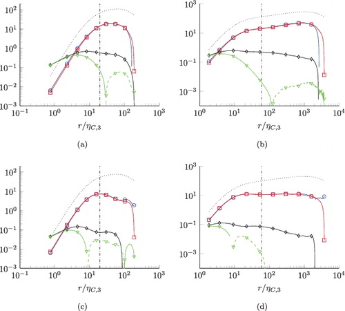
3.1. Even orders (N = 2, 4, 6)

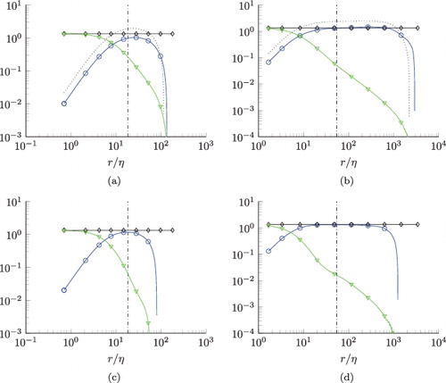
The balances of the second-order structure function equations are shown in Figure 2, where the longitudinal balance for D_{2, 0} is shown in Figure 2(a, b) and the transversal in Figure 2(c,d). The smaller Reynolds number case R0 corresponds to the left column, while the balances for R6 are depicted in the right column. Since we have normalised the terms with <ϵ >, both dissipation source terms E₁₁/ < ϵ > = E₂₂/ < ϵ > = 4/3 are constants over all r/η. As expected, the dissipation source terms balance the viscous terms in the viscous range, while they (nearly) balance the transport terms in the inertial range. Noticeably, the inertial range becomes broader with increasing Reynolds number in agreement with the notion of an increasing scale separation L/η. Consequently, the 4/5-law is more distinctive for the case R6, for which the viscous terms can be neglected in the inertial range. For R0 (Re_λ = 88), the viscous terms contribute to some extent to the balance in the inertial range. For N = 2, the pressure source terms vanish under the assumption of (local) isotropy and have therefore not been plotted. Considering the longitudinal equation, it is clearly seen that there is significant cancellation between the term ∂D_{3, 0}/∂r + 2D_{3, 0}/r and the term −4D_{1, 2}/r feeding into the equation as indicated by the dotted curve.

Figure 2. Balances of normalised second-order structure function equations N = 2. m = 2, n = 0 (a) and (b), m = 0, n = 2 (c) and (d). Left column: Re_λ = 88. Right column Re_λ = 754. Ratio λ/η is indicated by the vertical dash-dotted lines.

: transport terms, ⋄: dissipation source terms,

: viscous terms. Legend in Table 2. All terms are divided by ⟨ϵ⟩.

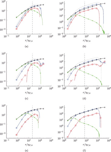
We find qualitative similar behaviour at the fourth order N = 4, as seen in Figure 3. The balances for D_{4, 0} are shown in Figure 3(a,b), for D_{2, 2} in Figure 3(c,d) and for D_{0, 4} in Figure 3(d,f). Since ⟨ϵ²⟩ and ν are the correct quantities to normalise the fourth-order structure functions in the viscous range, see Equation (14(14) ), we have normalised the terms with ⟨ϵ²⟩^6/8ν^1/2 with the abscissa r/η_{C, 4}. Again, this normalisation leads to a collapse of the viscous and dissipation source terms of the respective orders in the viscous range, where these two terms are dominant. The mixed pressure source term T_{2, 2}, which appears in Figure 3(c,d), has a different sign in the viscous range compared to the inertial range. However, this observation does not seem significant, as the pressure source terms are negligible in the viscous range. Unlike N = 2 in Figure 2, there are no r-independent terms in the inertial range. In the transverse equation for D_{0, 4}, the transport term is nearly balanced by the dissipation source term, while the pressure source terms are negligible, both for the smaller and the larger Reynolds number. Consequently, in the inertial range (18) For the mixed and longitudinal equation, the pressure source term contributes to the balance for the higher Reynolds number Re_λ = 754, which is not the case at the lower Reynolds number Re_λ = 88. However, this is somewhat deceiving, since there is significant cancellation in the transport term as in Figure 2, as indicated by the dotted lines.

Figure 3. Balances of normalised fourth-order structure function equations N=4. m = 4, n = 0 (a) and (b), m = 2, n = 2 (c) and (d), m = 0, n = 4 (e) and (f). Left column: Re_λ = 88. Right column Re_λ = 754. Ratio λ/η_{C, 4} is indicated by the vertical dash-dotted lines.

: transport terms,

: pressure source terms, ⋄: dissipation source terms,

: viscous terms. Legend in Table 2. Changes of signs are indicated by the dashed lines. All terms are divided by ⟨ϵ²⟩^6/8ν^1/2.

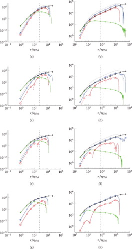
We show the sixth-order equations N = 6 in Figure 4, where the balance for D_{6, 0} can be found in Figure 4(a,b), D_{4, 2} in Figure 4(c,d), D_{2, 4} in Figure 4(e,f) and D_{0, 6} in Figure 4(g,h), where we have normalised the terms with ⟨ϵ³⟩^8/12ν and the abscissa with η_{C, 6} from Equation (15(15) ). Again, we observe mostly similar characteristics as for N = 4. In the viscous range, the dissipation source term and the viscous terms dominate and balance to leading order for all sixth-order equations. In the inertial range, the transport term of the transverse equation for D_{0, 6} is mostly balanced by the dissipation source term E_{0, 6}, i.e. (19) similarly to the fourth order where the transverse transport term was balanced by E_{0, 4} (cf. Equation (18(18) ) and Figure 3(e,f)). While the dissipation source terms are larger than the pressure source terms in the inertial range for all sixth-order balances, the ratio of dissipation source terms to pressure source terms decreases the more longitudinal the underlying structure function is: in the equation for D_{6, 0}, the pressure source terms are of the same order as the dissipation source terms, while T_{0, 6} is negligible compared to E_{0, 6} in the transverse equation. The mixed pressure source terms T_{4, 2} and T_{2, 4} exhibit a change of sign as indicated by the dashed lines from the viscous to the inertial range, as did the mixed pressure source term T_{2, 2} in the fourth-order equations. Finally, there is again cancellation in the transport terms of all but the transverse equation due to the contribution by the coupling to the other equations. As for N = 4, this is indicated by the dotted lines which are larger than the full transport terms in the inertial range.

Figure 4. Balances of normalised sixth-order structure function equations N=6. m = 6, n = 0 (a) and (b), m = 4, n = 2 (c) and (d), m = 2, n = 4 (e) and (f), m = 0, n = 6 (g) and (h). Left column: Re_λ = 88. Right column Re_λ = 754. Ratio λ/η_{C, 6} is indicated by the vertical dash-dotted lines.

: transport terms,

: pressure source terms, ⋄: dissipation source terms,

: viscous terms. Legend in Table 2. Changes of signs are indicated by the dashed lines. All terms are divided by ⟨ϵ³⟩^8/12ν.

We may conclude with general observations regarding the even-order balances: in the viscous range for all orders analysed above, the dissipation source terms and the viscous terms are dominant and balance each other. As discussed above, this is to be expected for all higher orders as well. In the inertial range, the transverse dissipation source terms E_0,N balance the transport terms for N = 2, 4, 6 and probably for higher even N as well. The solution of this approximate balance then feeds into the transverse and longitudinal equations, where these terms lead to significant cancellation in the longitudinal and mixed transport term. While this observation is certainly valid for all orders as well as for the range of Reynolds numbers examined here, it is not clear whether these findings generalise. Caution may be warranted because the pressure source terms become more important the higher the order and the more longitudinal the respective equation. In the inertial range, all terms but the viscous (which is negligible) can be approximated by a power law with the same exponent, at least for the orders and Reynolds numbers described above. Therefore, if one assumes a power law scaling for the odd-order structure functions in the inertial range, the longitudinal, mixed and transverse scaling exponents should be the same at the same order. Since all even-order dissipation source terms E_{m, n} are positive and consequently the transport terms , the odd-order structure functions in the inertial range are negative.

3.2. Odd orders (N = 3, 5, 7)

The balance of odd-order equations is presented in the following. The third-order longitudinal equations are shown in Figure 5(a,b) and the transverse in Figure 5(c,d). We have normalised the terms with ⟨ϵ^3/2⟩^5/6ν^1/4 and plotted them over η_{C, 3} as defined by Equation (15(15) ). In the viscous range, there is again the balance between dissipation source terms and viscous terms, which are dominant for the lower Reynolds number data R0, Re_λ = 88. However, for the higher Re_λ = 754 (R6), both the transport and the pressure source term are of the same order of magnitude for our data. This seems at odds with Equation (14(14) ), which was found to hold for odd orders as well, but could be resolved by plotting to smaller r, since the scaling of the terms for r → 0 as discussed in Section 2 is exact. Noticeably, the pressure and transport term also balance each other nearly perfectly. Indeed, the pressure source term balances the transport term not only in the viscous range, but also in the inertial range, where (20) i.e. the dissipation source terms may be neglected in the inertial range. As seen from the dotted lines, there is a large cancellation in the transport terms. Note that the findings of Grauer et al. [12] correspond to neglecting the pressure source terms T_{3, 0} and T_{1, 2} in Equation (20(20) ). The third-order structure function balances were previously examined by Hill and Boratav [8] using wind-tunnel data with Re_λ = 208 as well as DNS of isotropic turbulence with Re_λ = 82. Their results are in good agreement with our Figures 5. Noticeably, the two third-order pressure source terms have different signs, T_{3, 0} < 0 and T_{1, 2} > 0 differently to the even orders. Consequently, also the transport terms and , which implies 4D_{0, 4}/(3r) > ∂_rD_{2, 2} + (4/r)D_{2, 2} > 0 and ∂_rD_{4, 0} + (2/r)D_{4, 0} > (6/r)D_{2, 2} > 0 and the fourth-order structure functions are positive as required by definition.

Figure 5. Balances of normalised third-order structure function equations N=3. m = 3, n = 0 (a) and (b), m = 1, n = 2 (c) and (d). Left column: Re_λ = 88. Right column Re_λ = 754. Ratio λ/η_{C, 3} is indicated by the vertical dash-dotted lines.

: transport terms,

: pressure source terms, ⋄: dissipation source terms,

: viscous terms. Legend in Table 3. Changes of signs are indicated by the dashed lines. All terms are divided by ⟨ϵ^3/2⟩^5/6ν^1/4.

The N = 5 structure function equations are shown in Figure 6, where the terms are normalised with ⟨ϵ^5/2⟩^7/10ν^3/4 and the abscissa with η_{C, 5}. The longitudinal equation for D_{5, 0} is depicted in Figure 6(a,b), the mixed equation for D_{3, 2} in Figure 6(c,d) and the transverse D_{1, 4} in Figure 6(e,f). Similar to the N = 3 equations, the viscous terms and the dissipation source terms balance but would need to be plotted towards smaller r to be dominant at the higher Reynolds number Re_λ = 754. Both terms are negligible in the inertial range. The pressure source terms balance the transport terms over the full range for the longitudinal and transverse equations, cf. Figure 6(a,b,e,f). In the mixed equation, they also balance but have a zero-crossing at different r/η_{C, 5}. Thus, the balance between the pressure source term T_{3, 2} and the mixed transport term breaks down close to the respective zero-crossings. Besides the viscous range, there is again a large cancellation of terms in the transport terms as indicated by the dotted lines. Again, we find different signs for the pressure source terms: the transversal T_{1, 4} > 0 and mixed T_{3, 2} > 0, while the longitudinal T_{5, 0} < 0. With the respective signs of the transport terms, 6D_{0, 6}/(5r) > ∂_rD_{2, 4} + (6/r)D_{2, 4} > 0, ∂_rD_{4, 2} + (4/r)D_{4, 2} > 12D_{2, 4}/(3r) > 0 and ∂_rD_{6, 0} + (2/r)D_{6, 0} > (12/r)D_{4, 2} > 0.

Figure 6. Balances of normalised fifth-order structure function equations N=5. m = 5, n = 0 (a) and (b), m = 3, n = 2 (c) and (d), m = 1, n = 4 (e) and (f). Left column: Re_λ = 88. Right column Re_λ = 754. Ratio λ/η_{C, 5} is indicated by the vertical dash-dotted lines.

: transport terms,

: pressure source terms, ⋄: dissipation source terms,

: viscous terms. Legend in Table 3. Changes of signs are indicated by the dashed lines. All terms are divided by ⟨ϵ^5/2⟩^7/10ν^3/4.

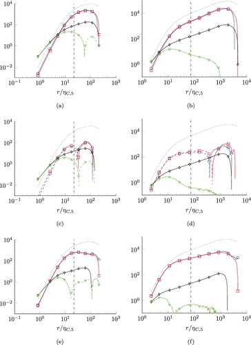
Finally, we look at the balances for N = 7 as seen in Figure 7. Specifically, the longitudinal balance for D_{7, 0} normalised with ⟨ϵ^7/2⟩^9/14ν^5/4 with abscissa r/η_{C, 7} is shown in Figure 7(a,b), the equally normalised balances for D_{5, 2} in Figure 7(c,d), for D_{3, 4} in Figure 7(e,f) and for D_{1, 6} in Figure 7(g,h). In the viscous range, there is the same balance of dissipation source terms and viscous terms as observed for the lower orders; while they dominate at the lower Reynolds number, the pressure source terms and the transport terms are of the same order of magnitude for the higher Reynolds number data-set R6. As was found for the lower odd orders, the pressure source terms and the transport terms balance for the full range of r/η_{C, 7} we have evaluated. Both the pressure source term and the transport term dominate the inertial range, where the dissipation source terms and the viscous terms can be neglected. Interestingly enough, only T_{5, 2} and the corresponding transport term in the equation for D_{5, 2} change their sign, while the other mixed pressure source term T_{3, 4} remains positive for all r/η_{C, 7}. Moreover comparing to N = 5, the change of sign of T_{5, 2} is at smaller r/η_{C, 7} compared to the zero-crossover of T_{3, 2} plotted over r/η_{C, 5}. For the seventh-order balance, we have T_{7, 0} < 0, a change of sign of T_{5, 2}, T_{3, 4} > 0 and T_{1, 6} > 0. Therefore, not only the transverse pressure source terms are negative in general (as one might have conjectured from the N = 3 balances), as are parts of the mixed. We expect similar characteristics at higher orders as well. With the signs of the transport terms in mind, one has 8D_{0, 8}/(7r) > ∂_rD_{2, 6} + (8/r)D_{2, 6} > 0, 18D_{2, 6}/(5r) > ∂_rD_{4, 4} + (6/r)D_{4, 4} > 0, ∂_rD_{6, 2} + (4/r)D_{6, 2} > 20D_{4, 4}/(3r) > 0 and ∂_rD_{8, 0} + (2/r)D_{8, 0} > (14/r)D_{6, 2} > 0.

Figure 7. Balances of normalised seventh-order structure function equations N=7. m = 7, n = 0 (a) and (b), m = 5, n = 2 (c) and (d), m = 3, n = 4 (e) and (f), m = 1, n = 6 (g) and (h). Left column: Re_λ = 88. Right column Re_λ = 754. Ratio λ/η_{C, 7} is indicated by the vertical dash-dotted lines.

: transport terms,

: pressure source terms, ⋄: dissipation source terms,

: viscous terms. Legend in Table 3. Changes of signs are indicated by the dashed lines. All terms are divided by ⟨ϵ^7/2⟩^9/14ν^5/4.

Let us briefly summarise the odd orders: for r → 0, again the dissipation source terms and viscous terms are dominant, if plotted towards small enough r. Consequently, the order-dependent viscous scales, Equation (15(15) ), are also valid for the odd orders, since the viscous terms and dissipation source terms balance. Indeed, the normalisation with η_{C, N} and u_{C, N} collapses the viscous and dissipation source terms in the viscous range for different Reynolds numbers (not easily seen from the figures). Noticeably, all odd-order dissipation source terms are negative while the corresponding even-order dissipation source terms are positive. Both contribute to the respective signs of the structure functions: the positive even-order dissipation source terms lead to negative odd-order structure functions, while the negative odd order dissipation source terms add to the positive even-order structure functions, albeit not much. In the inertial range, both the viscous and dissipation source terms can be neglected, so that to leading order the transport terms and the pressure source terms balance, as was also found by Gotoh and Nakano [11]. This is also in agreement with Yakhot's mean-field theory [5] applied to longitudinal and mixed equations with odd N. This leading-order balance in the inertial range is much better satisfied than the analogous balance of transport terms and dissipation source terms for the even orders, cf. the figures above. However, under the inertial range assumptions it is not possible to determine the solution of the even-order structure functions from these balances, since there are more unknown structure functions than equations. Finally, the dissipation source terms have a different scaling in the inertial range than the pressure source terms and the full transport terms, at least for balances other than the longitudinal in the fifth- and seventh-order equations. Nevertheless, since they are much smaller and can be neglected, power law behaviour of the even-order structure functions in the inertial range with equal scaling exponents seems plausible. There is one conflicting observation, though: if one approximates the dissipation source terms with a power law, then parts of the transport term (the dotted lines) can be approximated by a power law with same scaling exponent (except for N = 3). This result immediately contradicts the finding that the full transport terms approximately equal the pressure source terms which would have a different scaling exponent compared to the dissipation source terms except the longitudinal balances at N = 5 and 7. That is, even-order structure functions have the same inertial-range scaling exponents only if one neglects the pressure source terms or assumes that they have the same inertial-range scaling as the dissipation source terms.

4. Trace of structure function equations

In this section, we look at the balances of the traces of the structure function equations for N = 2 to 7. For the even-order equations, there is an even number of indices which are pairwise contracted leaving no free index resulting in scalar equations. For even N, we have (21) However for the odd-order equations, there remains a single index after contracting, resulting in a vector equation for the trace. As the separation vector r_i has been chosen to be aligned with the x₁-axis, only the 1-component of the vector equation does not vanish. Consequently, we define (22) Note that ⟨Δu₂[(Δu_i)²]^{(N − 1)/2}⟩ = 0 (N odd) due to isotropy, since we have aligned the separation vector r_i with the x₁-axis, i.e. r₂ = 0 and equally for the 3-component.

One can then express the trace of the general structure function tensor ⟨Δu_iΔu_j…⟩ in terms of the longitudinal, mixed and transverse structure functions D_{m, n} = ⟨(Δu₁)^m(Δu₂)ⁿ⟩. The resulting sums are listed in Table 4. The tabulated trace relations apply to any isotropic tensor that is symmetric under interchange of all indices, i.e. also to and , e.g. E_[4] = E_{4, 0} + 4E_{2, 2} + 8E_{0, 4}/3.

Table 4. Second to eighth-order structure function traces as defined by Equations (21(21) ) and  (22(22) ).

N = 2	D[2] = D2, 0 + 2D0, 2
N = 3	D[3] = D3, 0 + 2D1, 2
N = 4
N = 5
N = 6
N = 7
N = 8

We examine the trace equations for two reasons: first, the trace is invariant (i.e. independent of the coordinate system) for the even-order equations. Therefore, one finds for instance for N = 2 the mean of the pseudo-dissipation <ε > instead of the components <ε₁₁ > and <ε₂₂ >, cf. Equation (2(2) ). Similarly, at N = 4 one finds in the trace of the dissipation source term equation a term proportional to <ε² > + < ε_ijε_ji > instead of sums of the components < ε²₁₁ >, < ε²₂₂ > and < ε²₁₂ > (cf. Peters et al. [14]). That is, the higher moments of the pseudo-dissipation are found in consecutive equations stemming from the dissipation source terms of the structure function trace equations and not the longitudinal, mixed or transverse equations. Second, since the even-order trace is a scalar, one always has only a single equation for a single quantity at even N both in the viscous and inertial range, differently to the components equations. For the odd orders, one can project the trace equations in r_i-direction, but the resulting 1-components and the additional term D_22ii… depend on the coordinate system. The absolute magnitudes of odd-order traces as in Equation (22(22) ) are the magnitude of vectors and are therefore scalars.

Noticeably, the relations between the different orders as highlighted in Figure 1 and discussed in Section 2 above do not hold for the traces defined in Equations (21(21) ) and  (22(22) ). Consider the second order, N = 2. There, the trace of the transport term is (23) i.e. a similar coupling between the third- and second-order traces is found and similar relations are easily derived for the trace of transport terms in the higher even-order equations. However, for the third-order trace (24) and therefore there are additional terms in the odd-order trace of the transport terms which need to be closed. Again, similar additional terms are found for the trace of transport terms in all odd-order equations.

This implies that it is possible to directly integrate the transport term in the even-order trace equations: (25) In the inertial range, the last term on the r.h.s. can be neglected and the solution for the odd-order structure function trace then depends on the integrated sum of the traces of the dissipation source terms and pressure source terms. Again, a power law for D_[N+1], N even, can only be obtained if both E_[N] and T_[N] follow the same power law as well. All even N can be integrated in the viscous range by solving for the viscous term to determine the respective solutions if the dissipation source term is known, since both terms balance each other. One then obtains (26) or equivalently from an integration by parts (27) For r → 0, E_[N] = B_Nr^N−2 where B_N is a scalar, which then gives from both Equations (26(26) ) and  (27(27) ) (28) for the trace of even-order structure functions in the viscous range.

The integration of the trace of the fourth-order structure function equations was carried out by Peters et al. [14] both in the inertial and the viscous range. One can similarly proceed for higher orders N.

For odd orders in the inertial range, one has additional terms as seen from Equation (23(23) ) for N = 3 and similarly for higher odd orders. Thus, one needs to close these additional terms and then integrate in r resulting in a solution for D_[N+1] or compute the gradient and then project in r-direction. Then, one obtains (29) where D_11ii… = ⟨(Δu₁)²[(Δu_i)²]^{(N − 1)/2}⟩ and D_22ii… = ⟨(Δu₂)²[(Δu_i)²]^{(N − 1)/2}⟩. Note that because of N odd, E_[N] = E_1ii… and T_[N] = T_1ii…, differently to N even. One could then write due to (local) isotropy (30) In the viscous range, the balance reduces to (31) for odd N. In the viscous range, D_N = A_Nr^N where A_N is a scalar and consequently (32) which is consistent with the third-order solutions  (13(13) ).

4.1. Even orders

The balances for the traces of the structure functions for even orders as defined by Equation (21(21) ) were computed by summing up the individual even-order balances according to Table 4. The balance for the second-order trace equations normalised with ⟨ϵ⟩ is plotted over r/η and shown in Figure 8(a,b), while the balance of the N = 4 trace D_[4] normalised with ⟨ϵ²⟩^6/8ν^1/2 over r/η_{C, 4} and the N = 6 balance for D_[6] normalised with ⟨ϵ³⟩^8/12ν over r/η_{C, 6} are depicted in Figure 9(a,b) and Figure 10(a,b), respectively. Since the trace balances are the sum of the individual balances of Section 3.1, similar conclusions can be drawn. For all three even orders examined here, the trace of the dissipation source terms E_[N] balances the trace of the viscous source terms in the viscous range, where the traces of the pressure source terms T_[N] and transport terms can be neglected. If one then derives consecutive transport equations for E_[N], one finds that E_[N] ∼ ⟨ε^N/2⟩ν^{1 − N/2}r^{N − 2} in the viscous range as discussed in Section 2. In the inertial range, the trace of the viscous terms and the trace of the pressure source terms can be neglected to yield to leading order: (33) Noticeably, this balance is better satisfied at the lower Reynolds number Re_λ = 88. For that reason, one should be somewhat cautious when neglecting the trace of the pressure source terms at high Reynolds numbers and orders, although neglecting T_[N] at the higher Reynolds number for N = 6 seems justified. Approximating the traces in the inertial range with a power law would result in the same scaling exponent for E_[N], T_[N] and the transport term (cf. Figures 8–10) as was also found for the individual equations discussed above in Section 3.1.

Figure 8. Balances of normalised second-order structure function trace equation N=2. Left: Re_λ = 88. Right: Re_λ = 754. Ratio λ/η is indicated by the vertical dash-dotted lines.

: , ⋄: E_[2],

: . All terms are divided by ⟨ϵ⟩.

Figure 9. Balances of normalised fourth-order structure function trace equation N=4. Left: Re_λ = 88. Right: Re_λ = 754. Ratio λ/η_{C, 4} is indicated by the vertical dash-dotted lines.

: , ¿: T_[4], ⋄: E_[4],

: . All terms are divided by ⟨ϵ²⟩^6/8ν^1/2.

Figure 10. Balances of normalised sixth-order structure function trace equation N=6. Left: Re_λ = 88. Right: Re_λ = 754. Ratio λ/η_{C, 6} is indicated by the vertical dash-dotted lines.

: ,

: T_[6], ⋄: E_[6],

: . Changes of signs are indicated by the dashed lines. All terms are divided by ⟨ϵ^7/2⟩^8/12ν.

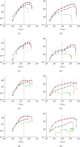
4.2. Odd orders

We show the balances for the odd-order trace equations for the third order, the fifth order and the seventh order in Figures 11–13, where we have normalised the traces as the individual equations discussed in Section 3.2. We find similar characteristics for the odd-order trace equations as for the respective longitudinal, mixed and transverse equations. While the trace of the dissipation source terms and the viscous terms dominate the trace of transport terms and pressure source terms in the viscous range for the lower Reynolds number case R0, all terms are of the same order of magnitude in the viscous range for the higher Reynolds number for all odd orders we have examined. Nevertheless, the balance of the trace of the viscous and dissipative terms holds also for the odd orders. In the inertial range, the trace of dissipation source terms can be neglected and the trace of pressure source terms and the transport terms are approximately equal. In Equation (29(29) ), E_[N] can be neglected, so that for all odd-order traces examined here (34) for all odd order traces examined here. Noticeably, Equation (34(34) ) also holds in the viscous range as does Equation (26(26) ), cf. Figures 11–13. Furthermore, the zero-crossing of the trace of transport and pressure source terms where their collapse is diminished moves to larger normalised r with increasing order and Reynolds number. Consequently, the approximation  (34(34) ) holds over a larger range of r with increasing order and Re_λ. Assuming power laws in the inertial range, the trace of dissipation source terms scales differently than both the trace of pressure source terms and transport terms, as seen from the figures.

Figure 11. Balances of normalised third-order structure function trace equation N = 3. Left: Re_λ = 88. Right: Re_λ = 754. Ratio λ/η_{C, 3} is indicated by the vertical dash-dotted lines.

: ,

: −T_[3], ⋄: −E_[3],

: . Changes of signs are indicated by the dashed lines. All terms are divided by ⟨ϵ^3/2⟩^5/6ν^1/4.

Figure 12. Balances of normalised fifth-order structure function trace equation N=5. Left: Re_λ = 88. Right: Re_λ = 754. Ratio λ/η_{C, 5} is indicated by the vertical dash-dotted lines.

: ,

: −T_[5], ⋄: −E_[5],

: . Changes of signs are indicated by the dashed lines. All terms are divided by ⟨ϵ^5/2⟩^7/10ν^3/4.

Figure 13. Balances of normalised seventh-order structure function trace equation N=7. Left: Re_λ = 88. Right: Re_λ = 754. Ratio λ/η_{C, 7} is indicated by the vertical dash-dotted lines.

: ,

: −T_[7], ⋄: −E_[7],

: . Changes of signs are indicated by the dashed lines. All terms are divided by ⟨ϵ^7/2⟩^9/14ν^5/4.

Figure A1. Normalised energy spectra E(κ)/(⟨ϵ⟩^2/3κ^−5/3) (a) and normalised dissipation spectra 2νκ²E(κ)/(⟨ϵ⟩η) (b) for R0 (○), R1 (□), R2 (⋄), R3 (▿), R4(▵), R5 (⋆) and R6 (+) plotted over κη. Higher Reynolds numbers are indicated by lighter shading.

5. Conclusions

We have computed balances of structure function equations and their traces up to the seventh order using DNS of homogeneous isotropic flow with Reynolds numbers up to Re_λ = 754.

For even orders, the dissipation source terms , which are related to correlations between velocity differences and the pseudo-dissipation, were found to be the dominant source terms. In the viscous range, they balance the viscous terms, while they balance the transport terms in the inertial range to leading order. Interestingly, there are as many equations as unknown structure functions in the inertial range at even orders, similarly to the K41 result for the second-order equations leading to the 4/5-law. That is, one can integrate the even-order equations under the inertial range assumptions and could solve for all odd-order structure functions, if the source terms were known. That is, one would obtain the odd-order structure functions as function of the source terms only. Again, the second order is very special, since the pressure source terms vanish due to local isotropy and the dissipation source terms can be written as ⟨ε⟩, i.e. become a one-point quantity independent of r, thus facilitating the integration. There are no such analogous results for higher even orders, since the pressure source terms do not vanish (but may be negligible at lower orders) and the dissipation source terms remain two-point quantities depending on r, thus prohibiting simple phenomenology such as K41. The coupling in the mixed and longitudinal equations contributes significantly to the structure function equation balances, to the effect that one could neglect also the dissipation source term in these equations for the orders examined here. However, the ratio of pressure source terms to the dissipation source terms T_{N, 0}/E_{N, 0} in the longitudinal equations increases with increasing order, so that these approximations may not be warranted at higher order N.

In the viscous range, the viscous terms and the dissipation source terms balance and one could proceed by deriving consecutive equations for the dissipation source terms. However, it is not possible to solve for the structure functions contained in the Laplacian in general, since the structure function equations are linearly dependent, with the exception of the second-order (and third-order) equations where the continuity equation provides an additional relation between D_{2, 0} and D_{0, 2} (as well as D_{3, 0} and D_{1, 2}). That is, there are no analogous relations at higher orders. Nevertheless, the exact viscous range solution for all even-order longitudinal equations as given by Equation (14(14) ) is known, although the corresponding C_{m, n} for mixed and transverse structure functions remain empirical.

On the other hand, odd orders are different inasmuch that there is one less equation than unknown structure functions under the inertial range assumptions after neglecting the viscous terms , even if the source terms were known. Noticeably, the pressure source terms are dominant in the odd-order equation balances and balance the transport terms nearly perfectly. Remarkably, this seems to hold even in the viscous range, where still the dissipation source terms balance the viscous terms as in the even-order equations. That is, the solution of odd-order structure functions in the viscous range is still determined by the dissipation source terms and indeed we have found an exact result for the third-order structure functions as given by Equation (13(13) ).

We have also evaluated the balances of the traces of the structure function equations up to the seventh order. The trace equations are of interest, because they contain the higher moments of the pseudo-dissipation in equations for the trace of dissipative source terms. For instance, the dissipation source term of the second- order trace equation equals the mean of the pseudo-dissipation ⟨ε⟩. Similarly, one finds the second moment ⟨ε²⟩ in the transport equation of the trace of fourth-order dissipative source terms, ⟨ε³⟩ in the transport equation of one of the source terms of the transport equation of the trace of sixth-order dissipative source terms and so on, cf. Peters et al. [14]. That is, these moments are not contained in the longitudinal, mixed or transverse equations but in the trace equations. The only exception is the second order, where due to isotropy ⟨ε₁₁⟩ = ⟨ε₂₂⟩ = ⟨ε⟩/3. But similar relations do not exist at higher orders. Since the trace is either a scalar for even orders or the 1-component of a vector for odd orders, one can always solve the trace equation in the inertial and viscous range if the source terms are known, as there is one equation for one unknown. However, there is no coupling via the transport terms between trace equations of N + 1 and N for N odd. That is, there is no system of trace equations as compared to the individual equations analogous to Figure 1 in the sense that one cannot compute the D_{[N + 1]} for odd N and insert them into the transport term of the even-order trace equations. Since the trace is the sum of the longitudinal, mixed and transverse structure functions, the trace balances are qualitatively similar to the individual balances. For even orders, the trace of dissipation source terms balances the trace of viscous terms in the viscous range and to leading order the trace of transport terms in the inertial range, while the pressure source terms are negligible. For odd orders, the dissipation source terms are negligible, while still balancing the trace of viscous terms for r → 0. However, the trace of pressure source terms balances the trace transport terms nearly perfectly both in the viscous and inertial range.

Acknowledgments

This work was supported by the European Research Council under the ERC Advanced Grant MILESTONE (‘Multi-Scale Description of Non-Universal Behavior in Turbulent Combustion’). The authors gratefully acknowledge the computing time granted by the JARA-HPC Vergabegremium provided on the JARA-HPC Partition part of the supercomputer JUQUEEN at the Forschungszentrum Jülich.

Disclosure statement

No potential conflict of interest was reported by the authors.

Additional information

Funding

European Research Council [grant number ERC-2015-AdG 695747].

Appendix. Data-set description

For the analysis carried out in the present paper, we use data from direct numerical simulation (DNS) of forced homogeneous isotropic turbulence with seven different sets of Taylor-based Reynolds numbers ranging from Re_λ = 88 to Re_λ = 754, where Re_λ = u_rmsλ/ν. λ denotes the Taylor scale , u_rms = ⟨u_iu_i/3 ⟩ is the root-mean-square velocity, ⟨k⟩ = ⟨u_iu_i⟩/2 the mean kinetic energy and ⟨ϵ⟩ =2ν ⟨s_ijs_ij⟩ the mean energy dissipation, where the strain tensor s_ij = (∂u_i/∂x_j + ∂u_j/∂x_i)/2. Angle brackets ⟨…⟩ denote ensemble averages over the full box and several timesteps spanning more than an integral turnover time after the simulation reached its statistically steady state. M denotes the number of timesteps used to compute the averages; the statistics were taken over a time period t_avg after the simulation has reached the steady state. The seven data-sets have been computed on the JUQUEEN supercomputer at Forschungszentrum Jülich using a pseudo-spectral code with MPI/OpenMP parallelisation. The three-dimensional Navier–Stokes equations were solved in rotational form, where all terms but the non-linear term were evaluated in spectral space. For a faster computation, the non-linear term is evaluated in physical space. The computational domain is a box with periodic boundary conditions and length 2π. Data-set R0 was initialised with the velocity field obeying a prescribed spectrum ∝κ⁴exp ( − 2(κ/κ₀)²) with random phases. Data-sets R1 to R6 were initialised by interpolating the final state of the next-lower data-set unto a finer mesh and changing the viscosity. For dealiasing, the scheme of Hou and Li [26] has been used; consequently, the largest resolved wavenumber κ_max < N/2. For the temporal advancement, a second-order Adams–Bashforth scheme is used in case of the non-linear term, while the linear terms are updated using a Crank–Nicolson scheme. To keep the simulation statistically steady, the stochastic forcing scheme of Eswaran and Pope [27] is applied. The 2DECOMP&FFT library [28] has been used for spatial decomposition and to perform the fast Fourier transforms. The only parameter varied to increase the Reynolds number is the viscosity ν; the forcing parameters have been held constant. The properties of the DNS cases can be found in Table A1. The normalised three-dimensional energy spectrum E(κ)/(⟨ϵ⟩^2/3κ^−5/3) is shown in Figure 14(a) for all seven data-sets and the corresponding normalised dissipation spectra 2νκ²E(κ)/(⟨ϵ⟩η) are shown in Figure 14(b). η = (ν³/ ⟨ϵ⟩ )^1/4 is the Kolmogorov length scale with corresponding time scale τ_η = (ν/ ⟨ϵ⟩ )^1/2. Both the normalised energy spectra and the normalised dissipation spectra collapse well. Assuming K41 scaling, the ratio E(κ)/(⟨ϵ⟩^2/3κ^−5/3) = const. = C_K in the inertial range, where C_k ≈ 1.62 from the data. This is in agreement with values reported in the literature, see, e.g. Ishihara et al. [29] or Gotoh et al. [30].

Table A1. Characteristic parameters of the DNS.

	R0	R1	R2	R3	R4	R5	R6
N	512	1024	1024	2048	2048	4096	4096
Reλ	88	119	184	215	331	529	754
ν	0.01	0.0055	0.0025	0.0019	0.0010	0.00048	0.00027
κmaxη	3.93	4.99	2.93	4.41	2.53	2.95	1.76
⟨k⟩	11.15	11.38	11.42	12.70	14.35	23.95	24.42
⟨ϵ⟩	10.78	11.04	10.30	11.87	12.55	28.51	26.54
η	0.0175	0.0111	0.0062	0.0049	0.0030	0.0014	0.00093
λ	0.322	0.238	0.166	0.143	0.107	0.064	0.050
L	1.02	0.94	0.97	1.01	0.97	1.02	1.18
τ	1.03	1.03	1.11	1.07	1.14	0.84	0.92
τη	0.031	0.022	0.016	0.013	0.009	0.004	0.0032
tavg/τ	100	30	30	10	10	2	3
M	189	62	61	10	10	6	6
Δt	1.4e-4	8.0e-5	8.0e-5	2.85e-5	2.75e-5	1.01e-5	1.01e-5

The seven data-sets were computed on a computational mesh with 512³ grid points for case R0 up to 4096³ grid points for case R6. L is the integral length scale, computed here using the three-dimensional energy spectrum (A1) and τ = ⟨k⟩/⟨ϵ⟩ the integral time scale. The integral length scale L is small compared to the size of the boxes in order to reduce the influence of the periodic boundary condition. Our data is well resolved with κ_maxη ≥ 1.7 for all seven data-sets, where κ_max is the largest resolved wavenumber. In turn, this also implies that the Reynolds number is not as high as other DNS with comparable mesh size reported in the literature.

References

- Kolmogorov AN. The local structure of turbulence in incompressible viscous fluid for very large Reynolds numbers. In: Doklady akademii nauk SSSR. Vol. 30, 1941. p. 299–303.
- Kolmogorov AN. Dissipation of energy in locally isotropic turbulence. In: Doklady akademii nauk SSSR. Vol. 32, 1941. p. 16–18.
- Monin AS, Yaglom AM. Statistical fluid mechanics II. Cambridge (MA): MIT Press; 1975.
- Rotta JC. Turbulente Strömungen: eine Einführung in die Theorie und ihre Anwendung. Vol. 8. Göttingen: Universitätsverlag Göttingen; 2010.
- Yakhot V. Mean-field approximation and a small parameter in turbulence theory. Phys Rev E. 2001;63:026307.
- Hill RJ. Equations relating structure functions of all orders. J Fluid Mech. 2001;434:379–388.
- Hill R. Exact second-order structure-function relationships. J Fluid Mech. 2002;468:317–326.
- Hill RJ, Boratav ON. Next-order structure-function equations. Phys Fluids. 2001;13:276.
- Kurien S, Sreenivasan KR. Dynamical equations for high-order structure functions, and a comparison of a mean-field theory with experiments in three-dimensional turbulence. Phys Rev E. 2001;64:056302.
- Nakano T, Gotoh T, Fukayama D. Roles of convection, pressure, and dissipation in three-dimensional turbulence. Phys Rev E. 2003;67:026316.
- Gotoh T, Nakano T. Role of pressure in turbulence. J Stat Phys. 2003;113:855–874.
- Grauer R, Homann H, Pinton JF. Longitudinal and transverse structure functions in high-Reynolds-number turbulence. New J Phys. 2012;14:063016.
- Yakhot V. Pressure-velocity correlations and scaling exponents in turbulence. J Fluid Mech. 2003;495:135–143.
- Peters N, Boschung J, Gauding M, et al. Higher-order dissipation in the theory of homogeneous isotropic turbulence. J Fluid Mech 2016;803:250–274.
- Frisch U. Turbulence: the legacy of AN Kolmogorov. Cambridge: Cambridge University Press.
- Hill RJ. Opportunities for use of exact statistical equations. J Turbul. 2006; 7. Available from: http://dx.doi.org/10.1080/14685240600595636
- Hill RJ. Applicability of Kolmogorov's and Monin's equations of turbulence. J Fluid Mech. 1997;353:67–81.
- Lesieur M. Turbulence in fluids. Dordrecht: Kluwer Academic Publishers; 1997.
- Oberlack M, Peters N. Closure of the two-point correlation equation as a basis for Reynolds stress models. Appl Sci Res. 1993;51:533–538.
- Thiesset F, Antonia R, Danaila L, et al. Kármán-Howarth closure equation on the basis of a universal eddy viscosity. Phys Rev E. 2013;88:011003.
- Schaefer P, Gampert M, Goebbert J, et al. Asymptotic analysis of homogeneous isotropic decaying turbulence with unknown initial conditions. J Turbul. 2011; 12. Available from: http://dx.doi.org/10.1080/14685248.2011.601313
- Boschung J, Gauding M., Hennig F, et al. Finite Reynolds number corrections of the 4/5 law for decaying turbulence. Phys Rev Fluids. 2016;1:064403.
- Siggia ED. Invariants for the one-point vorticity and strain rate correlation functions. Phys Fluids (1958–1988). 1981;24:1934–1936.
- Boschung J. Exact relations between the moments of dissipation and longitudinal velocity derivatives in turbulent flows. Phys Rev E. 2015;92:043013.
- Boschung J, Hennig F, Gauding M, et al. Generalised higher-order Kolmogorov scales. J Fluid Mech. 2016;794:233–251.
- Hou TY, Li R. Computing nearly singular solutions using pseudo-spectral methods. J Comput Phys. 2007;226:379–397.
- Eswaran V, Pope S. Direct numerical simulations of the turbulent mixing of a passive scalar. Phys Fluids. 1988;31:506–520.
- Li N, Laizet S. 2DECOMP & FFT-A highly scalable 2D decomposition library and FFT interface. In: Cray user group 2010 conference, Edinburgh. 2010. p. 1–13. Available from: http://www.2decomp.org/
- Ishihara T, Gotoh T, Kaneda Y. Study of high-Reynolds number isotropic turbulence by direct numerical simulation. Annu Rev Fluid Mech. 2009;41:165–180.
- Gotoh T, Watanabe T, Suzuki Y. Universality and anisotropy in passive scalar fluctuations in turbulence with uniform mean gradient. J Turbul. 2011; 12. Available from: http://dx.doi.org/10.1080/14685248.2011.631926