
 ?Mathematical formulae have been encoded as MathML and are displayed in this HTML version using MathJax in order to improve their display. Uncheck the box to turn MathJax off. This feature requires Javascript. Click on a formula to zoom.
ABSTRACT
The partially averaged Navier–Stokes (PANS) model, proposed in Girimaji [Partially-averaged Navier-Stokes model for turbulence: a Reynolds-averaged Navier-Stokes to direct numerical simulation bridging method. ASME J Appl Mech. 2006;73(3):413–421], can be used to simulate turbulent flows either as a RANS, LES or DNS. The PANS model includes which denotes the ratio of modelled to total kinetic energy. In RANS,
, and in DNS it goes to zero. In the present study we propose a new formulation for
based on the H-equivalence introduced by Friess et al. [Toward an equivalence criterion for hybrid RANS/LES methods. Int J Heat Fluid Flow. 2015;122:233–246]. In this formulation the expression of
is derived to mimic DES. This new formulation behaves very much like classic DES, even though the two formulations use different mechanisms to separate modelled and resolved scales. They show very similar performance in separated flows as well as in attached boundary layers. Moreover, the new formulation exhibits similar robustness features as DES.
1. Introduction
The PANS model was proposed by Girimaji [Citation1] and the PITM (Partially Integrated Transport Model) was proposed by Schiestel and Dejoan [Citation2], Chaouat and Schiestel [Citation3]. The critical parameter in both models is (it is sometimes called r in PITM). It is defined as the ratio of the modelled to the total turbulent kinetic energy:
(1)
(1) In DNS (Direct Numerical Solution), it tends to zero and in RANS (Reynolds-Averaged Navier–Stokes) it should be one. In LES (Large Eddy Simulation), the parameter takes values between zero and one. It is natural to link
to the mesh resolution and in that aim several proposals have been made on how to compute
. By seeking the smallest resolved length scale for a given
through dimensional analysis, Girimaji and Abdul-Hamid [Citation4] proposed one way to compute
:
(2)
(2) using
, the smallest grid cell size. Basara et al. also used
prescribed from Equation (Equation2
(2)
(2) ), however taking the geometric average
. Kenjeres and Hanjalic [Citation5] have made a slightly different proposal which reads
(3)
(3) Another way is to compute
from its very definition (Equation1
(1)
(1) ).
is then computed using the running average. The expression (Equation1
(1)
(1) ) shall hereafter be refered to as
, the observed
. More recently, Foroutan and Yavuzkurt [Citation6] derived an expression from the Kolmogorov energy spectrum which reads
(4)
(4) In [Citation7], the expression in Equation (Equation3
(3)
(3) ) was found to give far too small
. The form in Equation (Equation2
(2)
(2) ) and (Equation1
(1)
(1) ) were evaluated but it was found that a constant
in the LES region is superior.
The present paper is based on the work in [Citation8] where they derived a relation between DES and PITM. They showed that the DES model could be formulated using . They call this model an equivalent DES model. The relation between DES and PANS is used in the present work, but it is used the other way around: a new form of
is derived based on the DES model. In [Citation9] the form of
(new PANS, detailed in Section 2.1) was compared to DES. and the two models were found to give more or less identical results, particularly regarding first-order moments: velocity, skin friction coefficient
. In the present work the new PANS will be compared to the expression in Equation (Equation2
(2)
(2) ) (the old PANS using Δ=(ΔV)1/3) which in the literature is the most common way to compute
.
The paper is organised as follows. First, the form of is derived and analysed analytically. In the following section we present the numerical method. Then the new and old PANS are compared in three different flows (channel flow, hump flow and hill flow). Some conclusions are drawn in the final section.
2. The PANS model
The low-Reynolds number Partially-Averaged Navier–Stokes (LRN PANS, see [Citation10]) turbulence model reads
(5)
(5) where
denotes the material derivative. The damping functions are given by
(6)
(6) The functions
and
denote the ratio of modelled to total kinetic energy and modelled to total dissipation, respectively. For flows at high Reynolds numbers (as in the present work), the dissipation is modelled which means that
. In the PITM model,
and
.
2.1.  derived from the equivalence criterion
In [Citation8] a relation between and the grid step is derived, through the establishment of a statistical equivalence between DES and PITM. To that aim, they performed perturbation analyses about the equilibrium states, representing small variation of the energy partition. They did the analysis with and without considering inhomogeneity. That derivation is summarised here in a homogeneous framework, as a first step. Let us first consider the PANS/PITM equations. For equilibrium turbulence
where
, Equation (Equation5
(5)
(5) ) gives
(7)
(7) where
and
denote the diffusion term for k and ϵ, respectively. For local homogeneous turbulence (i.e.
), it can be written
(8)
(8) The quantities that are affected by the partition between modelled and resolved turbulence (i.e.
) in Equation (Equation8
(8)
(8) ) are γ, S, k and
.Footnote1 Differentiation of Equation (Equation8
(8)
(8) ), by considering infinitesimal perturbations
,
,
and
of the variables, yields:
(9)
(9) so that
(10)
(10) Equation (Equation10
(10)
(10) ) was derived for the PANS/PITM equations. Now we repeat the derivation for the DES equations. The differences between DES and PITM/PANS are that in DES (i)
is constant and (ii) the dissipation term in the equation for modelled energy k is replaced with
, i.e.
(11)
(11)
(12)
(12) Assuming
and local homogeneous turbulence gives
(13)
(13) We differentiate so that
(14)
(14) Equations (Equation9
(9)
(9) ) and (Equation14
(14)
(14) ) describe how
and ψ depend on variations in γ, S and k. The parameters
and ψ vary from
and 1 (RANS values), respectively, to
and
(LES values). Combining Equations (Equation9
(9)
(9) ) and (Equation14
(14)
(14) ) and integrating from RANS to LES conditions (
and ψ)
(15)
(15) By using the expression for
in Equation (Equation5
(5)
(5) ) (with
), and ensuring that
we finally get
(16)
(16) where ψ is given by Equation (Equation12
(12)
(12) ). This may be compared with the old formulations in Equations (Equation2
(2)
(2) ), (Equation3
(3)
(3) ) and (Equation4
(4)
(4) ). However, the present study focuses on a comparison between Equations (Equation2
(2)
(2) ) and (Equation16
(16)
(16) ).
2.2. Self-adaptivity properties of the new formulation of for PANS
In this section, we will distinguish (see Equation (Equation1
(1)
(1) )), the observed energy ratio, from
, the targeted (or prescribed) energy ratio. In the turbulent closure equations (i.e.in PANS, computing
),
is used, but nothing ever guarantees that this level of modelled energy will be exactly reached, see e.g. [Citation11]. This can be explained by the fact that
is a rough estimate, obtained under assumptions that are not always fully valid. Meanwhile,
can be obtained from postprocessing, using its definition in Equation (Equation1
(1)
(1) ).
If the targeted energy ratio, , is computed following Equation (Equation16
(16)
(16) ), and if we use the definition (which is rigorous in average)
(17)
(17) and the assumption that the whole dissipation is modelled, i.e.
(at high Reynolds number):
(18)
(18) then Equation (Equation16
(16)
(16) ) can be rewritten as:
(19)
(19) (note that, for sake of clarity, the form of
is here allowed to go negative). This implies that
is implicitly linked to
, in the following way: if
is lower (resp. higher) than a certain threshold value,
will increase (resp. decrease), leading dynamically to an increase (resp. decrease) of k and thus
.
Of course, this rough reasoning assumes that the resolved part of k ‘responds’ to those changes quickly enough to leave almost unaffected.
Thus, one can conclude that defining according to Equation (Equation16
(16)
(16) ) drives
towards a certain threshold (which may be more or less close to
). Such a feature is not intrinsic to approaches such as PITM or PANS, if some spectral law or Equations (Equation2
(2)
(2) ), (Equation3
(3)
(3) ) or (Equation4
(4)
(4) ) are used to determine
. It is actually intrinsic to Detached Eddy Simulation (DES), from which the present new formulation of
inherits this interesting property. This strategy may be interpreted as passive control, since it does not require the explicit computation of any extra quantity, such as
.
3. Numerical solver
An incompressible, finite volume code is used [Citation12]. The convective terms in the momentum equations are discretised using central differencing except for the hump flow where 95% is taken from CDS and 5% from the second-order upwind MUSCL scheme. Hybrid central/upwind is used for the k and ϵ equations. The Crank–Nicolson scheme is used for time discretisation of all equations. The numerical procedure is based on an implicit, fractional step technique with a multigrid pressure Poisson solver [Citation13] and a non-staggered grid arrangement.
The filtered momentum equations with an added turbulent viscosity read
(20)
(20) where the first term on the right side is the driving pressure gradient in the streamwise direction, which is used in the fully-developed channel flow simulations and for the hill flow.
4. Results
The new formulation of is evaluated and compared with the old formulation given in Equation (Equation2
(2)
(2) ). Herafter, they will be referred to as ‘new PANS’ and ‘old PANS’. The comparison is performed in three test cases: fully developed channel flow, the hump flow (see Figure ), and the hill flow (see Figure ).
Figure 1. The geometry of the hump.
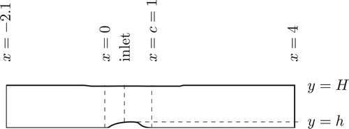
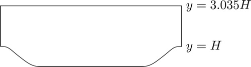
Figure 2. The geometry of the hill.
Ensemble-averaged quantities are plotted hereafter, i.e. they are averaged in time and over statistically homogeneous directions (which differ with flow cases).
4.1. Channel flow
The Reynolds number is defined as where δ denotes half channel height and
is the friction velocity. The streamwise, wall-normal and spanwise directions are denoted by x, y and z, respectively. The size of the domain is
,
and
. The mesh has
cells in the x−y−z directions. Periodic boundary conditions are used in the x and z directions. Therefore, these two directions are considered statistically homogeneous. A precursor DES computation is used as initial condition. The driving pressure gradient (first term on the right-hand side in Equation (Equation20
(20)
(20) ) is used with
. A lower limit of 0.05 is used when computing
from Equation (Equation16
(16)
(16) ).
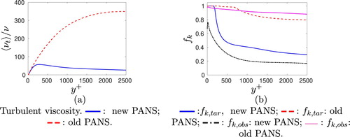
Figure presents the mean velocity and the turbulent kinetic energy profiles.As can be seen, the new PANS exhibits a small bump near ; otherwise it agrees well with the DNS profile. The predicted turbulent kinetic energies with both old and new PANS agree well with DNS for
. However, there is a big difference in how much turbulence is resolved and how much is modelled. For
, all turbulence is resolved by the new PANS model. In the old PANS model, all turbulence is modelled. The reason is found in Figure (b)): the old PANS predicts
in the entire region which means that the model is working in RANS mode. This is also seen in Figure (a)) in which it can be seen that the turbulent viscosity predicted by the old PANS is one-order magnitude larger than the new PANS model far from the wall. Furthermore, Figure (b)) shows that the new PANS exhibits a real plateau of
in the near-wall region, leading to a sharp switch from RANS to LES (at
, see insets). On the contrary, the old PANS does not switch to LES at all but stays in RANS mode in the entire channel. For both old and new PANS, the observed
is significantly different from the prescribed
, see Figure (b)). However, for the new PANS,
is smaller than
everywhere, but the profiles have a quite similar shape.
Figure 3. Channel flow, . Blue lines: new PANS; red lines: old PANS, see Equation (Equation2
(2)
(2) )
. Markers: DNS [Citation14].
![Figure 3. Channel flow, Reτ=5200. Blue lines: new PANS; red lines: old PANS, see Equation (Equation2(2) fk=Cμ−1/2ΔLt2/3,Lt=ktot3/2ε(2) ) Reτ=5200. Markers: DNS [Citation14].](/cms/asset/3a952e9f-f4b1-48be-b0d0-6237636c33b0/tjot_a_1641605_f0003_oc.jpg)
4.2. Hump flow
The Reynolds number of the hump flow is , based on the hump length, c=1, and the inlet mean velocity at the centreline,
. In the present simulations, the value of ρ, c and
have been set to unity. The configuration is given in Figure . Experiments were conducted by Greenblatt et al. [Citation15, Citation16]. The maximum height of the hump, h, and the channel height, H, are given by
and
, respectively. The mesh has
cells and is taken from the NASA workshop.Footnote2 The spanwise extent is set to
. The inlet is located at
and the outlet at
.
Figure 4. Channel flow. Viscosity and .
.
A periodic boundary condition is applied in the spanwise direction z. Therefore, this direction is considered statistically homogeneous. The inlet conditions (U, V, k and ϵ) are taken from a 2D RANS simulation using the AKN turbulence model [Citation17] coupled to the EARSM model [Citation18]. Synthetic isotropic fluctuations are superimposed on the 2D RANS velocity field. The synthetic fluctuations are scaled with the RANS shear stress profile. To reduce the inlet k, prescribed from 2D RANS, a commutation term
is used. For more detail on inlet synthetic fluctuations and the commutation term, see [Citation7]. A lower limit of 0.2 is used when computing
from Equation (Equation16
(16)
(16) ).
The simulations are initialised as follows [Citation19]: first the 2D RANS equations are solved. Anisotropic synthetic fluctuations, , are then superimposed to the 2D RANS field which gives the initial LES velocity field. In order to compute
, synthetic fluctuations,
, are computed plane-by-plane (y−z) in the same way as prescribing inlet boundary conditions. The synthetic fluctuations in the y−z planes are coupled with an asymmetric space filter
(21)
(21) where m denotes the index of the
location and
and
and
denote the grid size and the integral length scale, respectively (
).
Figures and compare predictions with experiments and, as can be seen, the new PANS is in a very good agreement with experiments, while the old PANS exhibits a significant discrepancy at . The predicted skinfrictions show a small bump near the inlet, and the reason is (at least partly) that a different RANS turbulence model (EARSM) was used in the 2D RANS simulations than the underlying RANS model in the PANS simulations. The backflow region is well predicted by both PANS models, but globally, the new PANS predicts the streamwise velocity far better than the old PANS.
Figure 5. Hump flow. Pressure coefficient and skinfriction. ![]()
![Figure 5. Hump flow. Pressure coefficient and skinfriction. Display full size: new PANS; Display full size: old PANS; markers: Experiments [Citation15, Citation16].](/cms/asset/4637e73b-70b0-4617-9f73-527b71672f2f/tjot_a_1641605_f0005_oc.jpg)
Figure 6. Hump flow. Streamwise velocities. ![]()
![Figure 6. Hump flow. Streamwise velocities. Display full size: new PANS; Display full size: old PANS; markers: Experiments [Citation15, Citation16].](/cms/asset/8f5c4815-4b5d-4b42-a770-ce24245494ea/tjot_a_1641605_f0006_oc.jpg)
Figure shows the turbulent viscosity for both models (note that the turbulent viscosities given by the old PANS have been multiplied by 0.1, for the sake of presentation). As in the channel flow, the turbulent viscosities predicted by the old PANS are an order of magnitude larger than those predicted by the new PANS. This means that the solution predicted by the old PANS is closer to RANS than to LES.
Figure 7. Hump flow. Turbulent viscosity. ![]()
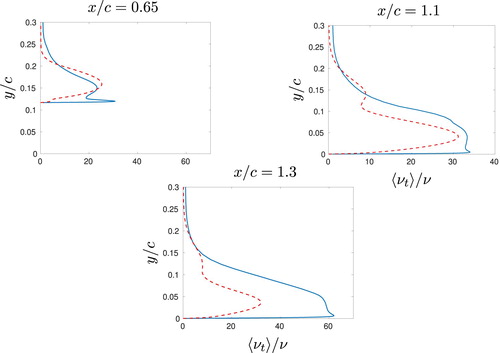
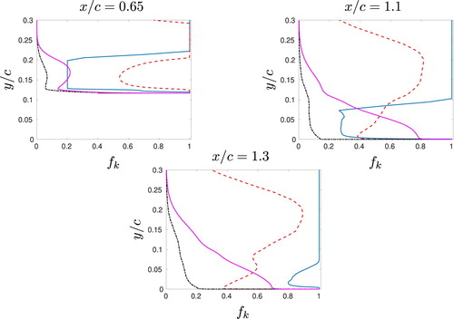
Figure presents and
for both old and new PANS at three locations,
and 1.3. The old PANS gives a much larger
(more RANS) than the new PANS as was noted above in Figure . The difference between the two model is largest in the attached flow region. Furthermore, for both approaches,
is significantly different from
,
being really low, although the flow is attached to the wall at all three locations. This may be due to the fact that the overall instability of the flow generates a big amount of fluctuations, thus increasing
, leading to a reduction of
.
Figure 8. Hump flow. ![]()
4.3. Hill flow
The domain is shown in Figure . The size of the domain is in the streamwise (x), wall-normal (y) and span-wise direction (z), respectively. The grid has
cells in the x, y and z direction. Periodic boundary conditions are used in the x and z directions. The z direction is considered statistically homogeneous. Slip conditions are prescribed at the upper wall. The Reynolds number is Re=10,600 based on the hill height and the bulk velocity at the top of the hill. An initial velocity field is prescribed from a 2D RANS solution with the correct bulk Reynolds number. Furthermore, the same technique for synthetic turbulence as for the hump flow, is used to add initial fluctuations. The bulk velocity is then kept constant by adjusting β in Equation (Equation20
(20)
(20) ) at each time step by ensuring that the sum of the forces at the wall (wall shear stress and pressure on the lower wall) balances the driving pressure gradient [Citation20, Citation21, Section 4.5]. A lower limit of 0.2 is used when computing fk from Equation (16).
Figure compares the velocity field with LES of [Citation22] and the agreement with the new PANS model is excellent.However, the old PANS model performs very poorly. The reason for the poor performance of the old PANS is seen in Figure (note that the viscosities of the old PANS have been multiplied by 0.1); the turbulent viscosity is one order of magnitude larger with the old PANS compared to the new PANS.
Figure 9. Hill flow. Velocities. ![]()
![Figure 9. Hill flow. Velocities. Display full size: new PANS; Display full size: old PANS; markers: LES [Citation22].](/cms/asset/9a32ea0e-a6f7-4a0f-a3a7-d3c5fcd33273/tjot_a_1641605_f0009_oc.jpg)
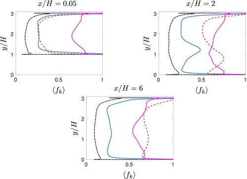
Figure compares profiles of and
for both PANS approaches. It is interesting to notice that at the top of the hill (
), the two
are close to each other, while their observed counterparts are significantly different: the new PANS is very well resolved, while the old one is closer to the RANS level. Further downstream, this global tendency is conserved, except that old and new PANS stray from each other, even after reattachment (
).
Figure 10. Hill flow. Turbulent viscosities. ![]()
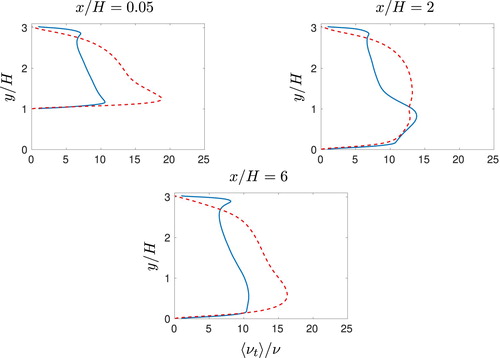
Figure 11. Hill flow. ![]()
5. Concluding remarks
A new formulation for prescribing has been presented. It has been found to perform much better than the standard form of
of [Citation4, Citation23]. It should, however, be mentioned that the standard form of
works much better when used in a four-equation turbulence model [Citation23] than in a two-equation model as in the present work, presumably because the four-equation closure contains more accurate near-wall physics.
The new formulation presented here, behaves very much like ‘classic DES’, as one can see in [Citation9], even though they use different mechanisms to separate modelled and resolved scales. In particular, they show very similar performance in separated flows, as well as in attached boundary layers.
Another interesting feature of the new PANS, is the robustness inherited from DES. As explained in Section 2.2, it behaves like a passive control device, in the sense that it does not require the explicit computation of the observed energy ratio .
So what is the advantage of using PANS instead of DES? One advantage is that PANS has a much stronger theoretical foundation than DES. PANS is rigorously derived whereas DES is an ad-hoc (but very successful) modification of a RANS model. Another advantage of PANS is that the modified partition between modelled and resolved turbulence due to non-uniform grids can be accounted for by adding a term in the k and momentum equations based on the gradient of [Citation7, Citation24]. Future work will focus on a thorough theoretical derivation of the relationship between
and the grid step, by accounting for inhomogeneity. Another test will consist of prescribing
with some more elaborate forms of DES, for instance Improved Delayed Detached Eddy Simulation (IDDES, see e.g. [Citation25, Citation26]).
Disclosure statement
No potential conflict of interest was reported by the authors.
Correction Statement
This article has been republished with minor changes. These changes do not impact the academic content of the article.
Notes
1. ϵ is independent of provided that no dissipation is resolved, which corresponds to
References
- Girimaji SS. Partially-averaged Navier-Stokes model for turbulence: a Reynolds-averaged Navier-Stokes to direct numerical simulation bridging method. ASME J Appl Mech. 2006;73(3):413–421. doi: 10.1115/1.2151207
- Schiestel R, Dejoan A. Towards a new partially integrated transport model for coarse grid and unsteady turbulent flow simulations. Theor Comp Fluid Dyn. 2005;18(6):443–468. doi: 10.1007/s00162-004-0155-z
- Chaouat B, Schiestel R. A new partially integrated transport model for subgrid-scale stresses and dissipation rate for turbulent developing flows. Phys Fluids. 2005;17(065106
- Girimaji SS, Abdul-Hamid KS. Partially-averaged Navier-Stokes model for turbulence: implementation and validation. AIAA paper 2005-0502. Reno, NV; 2005.
- Kenjeres S, Hanjalic K. LES, T-RANS and hybrid simulations of thermal convection at high ra numbers. Int J Heat Fluid Flow. 2006;27:800–810. doi: 10.1016/j.ijheatfluidflow.2006.03.008
- Foroutan H, Yavuzkurt S. A partially-averaged Navier-Stokes model for the simulation of turbulent swirling flow with vortex breakdown. Int J Heat Fluid Flow. 2014;50:402–416. doi: 10.1016/j.ijheatfluidflow.2014.10.005
- Davidson L. Zonal PANS: evaluation of different treatments of the RANS-LES interface. J Turbul. 2016;17(3):274–307. doi: 10.1080/14685248.2015.1093637
- Friess C, Manceau R, Gatski TB. Toward an equivalence criterion for hybrid RANS/LES methods. Int J Heat Fluid Flow. 2015;122:233–246.
- Davidson L, Friess C. The PANS and PITM model: a new formulation of fk. In Proceedings of 12th international ERCOFTAC symposium on engineering turbulence modelling and measurements (ETMM12), Montpelier, i France 26–28 September; 2018.
- Ma J, Peng S-H, Davidson L, et al. A low Reynolds number variant of partially-averaged Navier-Stokes model for turbulence. Int J Heat Fluid Flow. 2011;32(3):652–669. doi: 10.1016/j.ijheatfluidflow.2011.02.001
- Fadai-Ghotbi A, Friess C, Manceau R, et al. A seamless hybrid rans-les model based on transport equations for the subgrid stresses and elliptic blending. Phys Fluids. 2010;22(5):055104. doi: 10.1063/1.3415254
- Davidson L, Peng S-H. Hybrid LES-RANS: a one-equation SGS model combined with a k−ω for predicting recirculating flows. Int J Numer Methods Fluids. 2003;43(9):1003–1018. doi: 10.1002/fld.512
- Emvin P. The full multigrid method applied to turbulent flow in ventilated enclosures using structured and unstructured grids [PhD thesis]. Göteborg: Department of Thermo and Fluid Dynamics, Chalmers University of Technology; 1997.
- Lee M, Moser RD. Direct numerical simulation of turbulent channel flow up to Reτ≈5200. J Fluid Mech. 2015;774:395–415. doi:10.1017/jfm.2015.268
- Greenblatt D, Paschal KB, Yao C-S, et al. A separation control CFD validation test case. Part 1: baseline & steady suction. AIAA-2004-2220; 2004.
- Greenblatt D, Paschal KB, Yao C-S, et al. A separation control CFD validation test case part 1: zero efflux oscillatory blowing. AIAA-2005-0485; 2005.
- Abe K, Kondoh T, Nagano Y. A new turbulence model for predicting fluid flow and heat transfer in separating and reattaching flows – 1. Flow field calculations. Int J Heat Mass Transfer. 1994;37(1):139–151. doi:10.1016/0017-9310(94)90168-6
- Wallin S, Johansson AV. A new explicit algebraic Reynolds stress model for incompressible and compressible turbulent flows. J Fluid Mech. 2000;403:89–132. doi: 10.1017/S0022112099007004
- Davidson L. Zonal detached eddy simulation coupled with steady rans in the wall region. In ECCOMAS MSF 2019 thematic confernence, minisyposium ‘Current trends in simulation and modelling of turbulent flows. MS devoted to 80th birthday of Prof. Kemo Hanjalic’. September 18th–20th, 2019 – Sarajevo, Bosnia and Herzegovina; 2019.
- Irannezhad M. DNS of channel flow with finite difference method on a staggered grid [Msc thesis]. Göteborg: Division of Fluid Dynamics, Department of Applied Mechanics, Chalmers University of Technology; 2006.
- Orlandi P. Fluid flow phenomena – a numerical toolkit. Dordrecht: Kluwer Academic Publishers; 2000.
- Breuer M, Peller N, Rapp C, et al. Flow over periodic hills – numerical and experimental study in a wide range of Reynolds numbers. Comput Fluids. 2009;38:433–457. doi:10.1016/j.compfluid.2008.05.002
- Basara B, Krajnović S, Girimaji S, et al. Near-wall formulation of the partially averaged Navier Stokes turbulence model. AIAA J. 2011;49(12):2627–2636. doi: 10.2514/1.J050967
- Girimaji SS, Wallin S. Closure modeling in bridging regions of variable-resolution (VR) turbulence computations. J Turbul. 2013;14(1):72–98. doi:10.1080/14685248.2012.754893
- Shur ML, Spalart PR, Strelets MK, et al. A hybrid rans-les approach with delayed-des and wall-modelled les capabilities. Int J Heat Fluid Flow. 2008;29(6):1638–1649. doi: 10.1016/j.ijheatfluidflow.2008.07.001
- Gritskevich MS, Garbaruk AV, Schütze J, et al. Development of ddes and iddes formulations for the k-ω shear stress transport model. Flow Turbul Combust. 2012;88(3):431–449. doi: 10.1007/s10494-011-9378-4