Improving LES with OpenFOAM by minimising numerical dissipation and use of explicit algebraic SGS stress model

ABSTRACT

There is a rapidly growing interest in using general-purpose CFD codes based on second-order finite volume methods for Large-Eddy Simulation (LES) in a wide range of applications, and in many cases involving wall-bounded flows. However, such codes are strongly affected by numerical dissipation and the accuracy obtained for typical LES resolutions is often poor. In the present study, we approach the problem of improving the LES capability of such codes by reduction of the numerical dissipation and use of an anisotropy-capturing subgrid-scale (SGS) stress model. The latter is of special importance for wall-resolved LES with resolutions where the SGS anisotropy can be substantial. Here we use the Explicit Algebraic (EA) SGS model [Marstorp L, Brethouwer G, Grundestam O, et al. Explicit algebraic subgrid stress models with application to rotating channel flow. J Fluid Mech. 2009;639:403–432], and comparisons are made for channel flow at friction Reynolds numbers up to 934 with the dynamic Smagorinsky model. The numerical dissipation is reduced by using an OpenFOAM based custom-built flow solver that modifies the Rhie and Chow interpolation and allows to control and minimise its effects without causing numerical instability (in viscous, fully turbulent flows). Different resolutions were used and large improvements of the LES accuracy were demonstrated for skin friction, mean velocity and other flow statistics by use of the new solver in combination with the EA SGS model. By reducing the numerical dissipation and using the EA SGS model the resolution requirements for wall-resolved LES can be significantly reduced.

KEYWORDS:

• Large-eddy simulation
• wall-bounded flows
• OpenFOAM
• SGS modelling

1. Introduction

There is a rapidly growing interest in using general-purpose commercial and open-source CFD codes for large-eddy simulation (LES) for research and development purposes in academia and industry [1–4]. One of these general-purpose CFD codes often used for LES is the open-source code OpenFOAM, see e.g. [5,6]. A particular challenge for these CFD codes is LES of turbulent boundary layers over solid walls and other surfaces, which are often present in applications, because of the complex physics related to small-scale dynamics, which put strict demands on the grid resolution used. Near-wall modelling relaxes the resolution requirement for LES of high Reynolds number wall-bounded flows, but introduces additional modelling uncertainties [7–9]. Even with this approach, high Reynolds number external flows, e.g. around full-scale airplanes, are out of reach for several decades [10]. Wall-resolved LES avoids some of the modelling uncertainties, but it requires mesh resolutions in terms of inner viscous wall scaling resulting in a rapid increase of the computational effort with the Reynolds number. Wall-resolved LES of moderately high Reynolds number turbulent flows is nevertheless becoming feasible due to the growth of computational resources [11,12]. However, such a LES is sensitive to the numerical algorithm. Rezaeiravesh and Liefvendahl [11] carried out LES of turbulent channel flow with OpenFOAM and concluded that the numerical errors have a large influence on the accuracy of the predictions. The importance of the numerical algorithm in LES was also pointed out by e.g. Vuorinen et al. [13], Breuer [14], Piomelli [7]. There have been some efforts to improve the numerical accuracy of OpenFOAM, for example, Vuorinen et al. [13] introduced a low-dissipative time integration scheme.

In addition to the numerical algorithm, also the subgrid-scale (SGS) stress model has an important influence on the accuracy of a LES, if the numerical dissipation is small enough to reveal the major part of the flow dynamics. The importance of developing realisaable, physically consistent closures has been stressed by Silvis et al. [15], who proposed and tested a new eddy-viscosity SGS model based on the vortex stretching mechanism. In particular, for wall-bounded flows, there is potential for SGS model improvements in the near-wall region because there the scale separation is inherently limited and the turbulent anisotropy persists down to the smallest scales. Piomelli et al. [16] and Rouhi et al. [17] have focused on the development and testing of a subfilter-scale model that enables LES of wall-bounded flows with coarse grids. The study by Rasam et al. [18] shows the importance of correctly modelling the near-wall anisotropy of the turbulence in LES when the resolution becomes coarse. It is therefore natural to investigate the possible advantages offered by anisotropy-capturing SGS models.

An anisotropy-capturing SGS model, here referred to as the Explicit Algebraic Model (EAM), has been developed by Marstorp et al. [19]. This model was recently used by Montecchia et al. [20] for LES of turbulent channel flow with a pseudo-spectral code. The results showed substantial improvements with the EAM as compared to a dynamic Smagorinsky model (DSM) [21,22], for a wide range of friction Reynolds numbers up to 5200. Predictions of both the mean velocity profile and Reynolds stress distributions were significantly better with the EAM, especially at coarse resolutions. It was shown that this was related to a more correct description of the SGS anisotropy, which gives a considerable contribution to the flow dynamics in the viscous sublayer and the buffer region even at rather fine LES resolutions. In a pseudo-spectral code [20] LES with the DSM overestimated the Reynolds stress anisotropy, while LES with the EAM produces results closer to DNS from the buffer region up to the outer region, with a reasonable prediction of the inner peak amplitude for the streamwise normal stress. The DSM can be considered as an isotropic model since the SGS viscosity ${\nu }_{\mathrm{S}\mathrm{G}\mathrm{S}}$ is direction-independent. Rasam et al. [23] applied the EAM and the DSM in LES of the flow over periodic hills and also obtained substantial improvements with the EAM in this more complex flow case with separation. Instead of using a high-order code they used a general-purpose finite volume code for the LES but they did not consider the influence of the numerical algorithm on the results.

In this study, we are interested in LES of wall-bounded flows with the general-purpose code OpenFOAM because this code has been used in a wide range of applications. Rezaeiravesh and Liefvendahl [11] carried out an extensive investigation of LES of turbulent channel flow with OpenFOAM using various resolutions. They concluded that a very fine resolution is needed to obtain accurate results; the recommended cell size in the spanwise and streamwise direction is $(\mathrm{\Delta }{x}^{+},\mathrm{\Delta }{z}^{+})\approx (17,10)$, which is about twice the cell size of a typical DNS of turbulent channel flow [24]. Using such a fine resolution is obviously not satisfactory since it makes wall-resolved LES of higher Reynolds number wall-bounded flows with OpenFOAM computationally extremely expensive.

The principal aim of our work is therefore to reduce the computation costs of LES of wall-bounded flows with OpenFOAM and thereby increase the applicability of OpenFOAM in academic and industrial research. We address numerical and modelling aspects since both are important, as discussed above, for relaxing the resolution requirements of wall-resolved LES. Cadieux et al. [25], for instance, have shown how substantial numerical dissipation in a low-order solver can contaminate the results. In cases of significantly under-resolved LES, Cadieux et al. claimed that the results can be re-interpreted as implicit LES. To this end, the numerical dissipation is reduced by partial removal of the Rhie and Chow (R&C) interpolation and the EAM is implemented in a new version of OpenFOAM. We then investigate the impact of the reduction of numerical dissipation as well as the impact of the SGS modelling in LES of turbulent channel flow at friction Reynolds numbers ${\mathrm{R}\mathrm{e}}_{\tau }=u_{\tau }h/\nu =550$ and 934. Turbulent channel flow is a suitable test case because the numerical details and SGS modelling have a pronounced effect on LES of this case. In fact, our study underlines once more the significance of numerical and modelling aspects for LES of wall-bounded flows. We demonstrate that the reduced numerical dissipation and better SGS modelling produce significant improvements in wall-resolved LES so that also acceptable results can be obtained at coarser resolutions. This leads to substantial savings in the computational costs. The present results are naturally of importance for LES of wall-bounded flows with OpenFOAM, but they should also be of interest for LES of other flows, for example, with free shear layers, and LES with other low-order order numerical codes. Moreover, they give an indication of the resolution required in LES of other flows involving boundary layers.

The outline of the paper is as follows: Model descriptions are given in Section 2. The different aspects of the numerical implementation and the effect of minimising the numerical dissipation are presented in Section 3. A new EAM improvement, related to the conditions near the wall, is given in Section 4. Results for the prediction of skin friction, mean velocity profiles, statistics as well as spectra are presented in Section 5. Different grid resolutions are used and comparisons are made for LES with EAM, the DSM and no-model (NM). Some concluding remarks are given in Section 6. An appendix is included with more code-related implementation aspects, and one with some comments on the influence of errors caused by the time discretization on the statistics.

2. Model description

The governing equations in LES are the filtered, non-dimensional Navier–Stokes equations, which for an incompressible flow read (where $\widetilde{.}$ denotes filtered quantity): (1) $\frac{\mathrm{\partial }{\tilde{u}}_i}{\mathrm{\partial }{x}_i}=0;\frac{\mathrm{\partial }{\tilde{u}}_i}{\mathrm{\partial }t}+\frac{\mathrm{\partial }{\tilde{u}}_i{\tilde{u}}_j}{\mathrm{\partial }{x}_j}=-\frac{\mathrm{\partial }\tilde{p}}{\mathrm{\partial }{x}_i}+\frac{1}{\mathrm{R}\mathrm{e}}\frac{{\mathrm{\partial }}^2{\tilde{u}}_i}{\mathrm{\partial }{x}_j\mathrm{\partial }{x}_j}-\frac{\mathrm{\partial }{\tau }_{ij}}{\mathrm{\partial }{x}_j}$(1) where the filtering operation is performed implicitly. Here ${\tau }_{ij}$ is the subgrid-scale stress tensor, defined as (2) ${\tau }_{ij}=\widetilde{u_i{u}_j}-{\tilde{u}}_i{\tilde{u}}_j$(2) which represents an unknown part in the filtered equations that needs to be modelled.

2.1. Explicit algebraic SGS model (EAM)

In wall-bounded flows anisotropic effects of turbulence are noticeable and they persist to relatively small scales in the proximity of the wall.

In the Explicit Algebraic SGS model (EAM), anisotropy is properly considered and evaluated at the SGS level. The SGS and total anisotropy tensors are defined as follows: (3) $a_{ij}^{\mathrm{S}\mathrm{G}\mathrm{S}}=\frac{⟨{\tau }_{ij}⟩}{⟨K_{\mathrm{S}\mathrm{G}\mathrm{S}}⟩}-\frac{2}{3}{\delta }_{ij},a_{ij}=\frac{⟨\widetilde{u_i}\widetilde{u_j}⟩+⟨{\tau }_{ij}⟩}{K_{\mathrm{R}\mathrm{E}\mathrm{S}}+⟨K_{\mathrm{S}\mathrm{G}\mathrm{S}}⟩}-\frac{2}{3}{\delta }_{ij}$(3) where $K_{\mathrm{S}\mathrm{G}\mathrm{S}}={\tau }_{kk}/2$ and $K_{\mathrm{R}\mathrm{E}\mathrm{S}}=⟨\widetilde{u_k}\widetilde{u_k}⟩/2$ are the SGS and resolved parts of the turbulence kinetic energy, respectively, and $⟨.⟩$ is the average in time and in the homogeneous directions.

In the same spirit as Reynolds stress-based models for RANS, the model here discussed is called Explicit Algebraic SGS stress model (EAM). The EAM was developed by Marstorp et al. [19] and is similar to the EARSM by Wallin and Johansson [26]. The EAM is based on a modelled transport equation of the SGS stresses and on the assumption that the advection and diffusion of the SGS stress anisotropy are negligible.

The model formulation is given by (4) ${\tau }_{ij}=\frac{2}{3}{\delta }_{ij}{K}_{\mathrm{S}\mathrm{G}\mathrm{S}}+\underset{`\mathrm{e}\mathrm{d}\mathrm{d}\mathrm{y}-\mathrm{v}\mathrm{i}\mathrm{s}\mathrm{c}\mathrm{o}\mathrm{s}\mathrm{i}\mathrm{t}\mathrm{y}\text{'}\mathrm{t}\mathrm{e}\mathrm{r}\mathrm{m}}{\underbrace{{\text{β}}_1{K}_{\mathrm{S}\mathrm{G}\mathrm{S}}{\tilde{S}}_{ij}^{\ast }}}+\underset{\mathrm{n}\mathrm{o}\mathrm{n}-\mathrm{l}\mathrm{i}\mathrm{n}\mathrm{e}\mathrm{a}\mathrm{r}\mathrm{c}\mathrm{o}\mathrm{n}\mathrm{t}\mathrm{r}\mathrm{i}\mathrm{b}\mathrm{u}\mathrm{t}\mathrm{i}\mathrm{o}\mathrm{n}}{\underbrace{{\text{β}}_4{K}_{\mathrm{S}\mathrm{G}\mathrm{S}}({\tilde{S}}_{ik}^{\ast }{\tilde{\mathrm{\Omega }}}_{kj}^{\ast }-{\tilde{\mathrm{\Omega }}}_{ik}^{\ast }{\tilde{S}}_{kj}^{\ast })}}$(4) where ${\tilde{S}}_{ij}^{\ast }$ and ${\tilde{\mathrm{\Omega }}}_{ij}^{\ast }$ are the filtered strain and rotation-rate tensors normalised by $1/{\tau }^{\ast }$, the inverse of the SGS turbulence time scale. The filtered strain and rotation-rate tensors are respectively defined as follows: (5) ${\tilde{S}}_{ij}=\frac{1}{2}\left(\frac{\mathrm{\partial }{\tilde{u}}_i}{\mathrm{\partial }{x}_j}+\frac{\mathrm{\partial }{\tilde{u}}_j}{\mathrm{\partial }{x}_i}\right),{\tilde{\mathrm{\Omega }}}_{ij}=\frac{1}{2}\left(\frac{\mathrm{\partial }{\tilde{u}}_i}{\mathrm{\partial }{x}_j}-\frac{\mathrm{\partial }{\tilde{u}}_j}{\mathrm{\partial }{x}_i}\right)$(5) The second term on the right-hand-side of Equation (4(4) ${\tau }_{ij}=\frac{2}{3}{\delta }_{ij}{K}_{\mathrm{S}\mathrm{G}\mathrm{S}}+\underset{`\mathrm{e}\mathrm{d}\mathrm{d}\mathrm{y}-\mathrm{v}\mathrm{i}\mathrm{s}\mathrm{c}\mathrm{o}\mathrm{s}\mathrm{i}\mathrm{t}\mathrm{y}\text{'}\mathrm{t}\mathrm{e}\mathrm{r}\mathrm{m}}{\underbrace{{\text{β}}_1{K}_{\mathrm{S}\mathrm{G}\mathrm{S}}{\tilde{S}}_{ij}^{\ast }}}+\underset{\mathrm{n}\mathrm{o}\mathrm{n}-\mathrm{l}\mathrm{i}\mathrm{n}\mathrm{e}\mathrm{a}\mathrm{r}\mathrm{c}\mathrm{o}\mathrm{n}\mathrm{t}\mathrm{r}\mathrm{i}\mathrm{b}\mathrm{u}\mathrm{t}\mathrm{i}\mathrm{o}\mathrm{n}}{\underbrace{{\text{β}}_4{K}_{\mathrm{S}\mathrm{G}\mathrm{S}}({\tilde{S}}_{ik}^{\ast }{\tilde{\mathrm{\Omega }}}_{kj}^{\ast }-{\tilde{\mathrm{\Omega }}}_{ik}^{\ast }{\tilde{S}}_{kj}^{\ast })}}$(4) ) is an eddy-viscosity term responsible for SGS dissipation, whereas the third term accounts for anisotropic effects of SGS stresses and models the disalignment of the SGS stress and resolved strain-rate tensor. The ${\text{β}}_1$ and ${\text{β}}_4$ coefficients are given by (6) ${\text{β}}_1=-\frac{33}{20}\frac{9c_1/4}{\left[\right(9c_1/4{)}^2+|{\tilde{\mathrm{\Omega }}}^{\ast }{|}^2]},{\text{β}}_4=-\frac{33}{20}\frac{1}{\left[\right(9c_1/4{)}^2+|{\tilde{\mathrm{\Omega }}}^{\ast }{|}^2]}$(6) where $|{\tilde{\mathrm{\Omega }}}^{\ast }|=(2{\tau }^{{\ast }^2}{\tilde{\mathrm{\Omega }}}_{ij}{\tilde{\mathrm{\Omega }}}_{ij}{)}^{1/2}$.

The unknown quantities $K_{\mathrm{S}\mathrm{G}\mathrm{S}}$ and ${\tau }^{\ast }$ are dynamically computed. Here the SGS kinetic energy is modelled in terms of the squared Smagorinsky velocity scale $\mathrm{\Delta }|\tilde{S}|$ [27]: (7) $K_{\mathrm{S}\mathrm{G}\mathrm{S}}=c{\tilde{\mathrm{\Delta }}}^2|\tilde{S}{|}^2$(7) where $\tilde{\mathrm{\Delta }}=\sqrt[3]{\mathcal{V}}$ is the filter scale based on $\mathcal{V}$, the volume of a computational cell; $|\tilde{S}|=(2{\tilde{S}}_{ij}{\tilde{S}}_{ij}{)}^{1/2}$, and c is a dynamically computed parameter, described in the following way: (8) $c=\frac{1}{2}\frac{⟨|\mathcal{L}\mathcal{M}|⟩}{⟨\mathcal{M}\mathcal{M}⟩}$(8) where $\mathcal{L}=\widehat{{\stackrel{~}{u}}_i{\stackrel{~}{u}}_i}-\widehat{{\stackrel{~}{u}}_i}\widehat{{\stackrel{~}{u}}_i}$ and $\mathcal{M}={\widehat{\stackrel{~}{\mathrm{\Delta }}}}^2|{\widehat{\stackrel{~}{S}}}_{ij}{|}^2-\stackrel{ˆ}{{\tilde{\mathrm{\Delta }}}^2|{\tilde{S}}_{ij}{|}^2}$ The quantities with $\widehat{.}$ are test-filtered quantities. By the $⟨.⟩$ operation the values are interpolated from their respective cells to the faces, and a local average is computed from the faces belonging to a cell. Here we will use $\widehat{\stackrel{~}{\mathrm{\Delta }}}=2\tilde{\mathrm{\Delta }}$. The expression for c is a direct consequence of EAM SGS formulation. In wall-bounded flows, the dynamic procedure is essential in order to maintain a reasonable accuracy of the quantities close to the wall and replaces the need for additional near-wall correction methods. In contrast to DSM where two tensors are employed (${\mathcal{L}}_{ij}$ and ${\mathcal{M}}_{ij}$, see [22]), the dynamic procedure applied for EAM is based on the scale-similarity of the SGS stress tensor, and requires only two scalars to be evaluated resulting in fewer terms to compute (see expression (8(8) $c=\frac{1}{2}\frac{⟨|\mathcal{L}\mathcal{M}|⟩}{⟨\mathcal{M}\mathcal{M}⟩}$(8) )). The computational cost of the following LES with EAM is thereby less than that with DSM. The resulting wall-clock time for each timestep for the EAM was found to be about $18\mathrm{\%}$ shorter than for the DSM. In both the OpenFOAM implementations of the EAM and DSM the dynamic coefficient is clipped in order to avoid negative values for the $K_{\mathrm{S}\mathrm{G}\mathrm{S}}$ and the eddy-viscosity ${\nu }_{\mathrm{S}\mathrm{G}\mathrm{S}}$.

Once c is computed, it is possible to obtain the coefficient $c_1$ and the SGS time scale ${\tau }^{\ast }$, which according to [19] are given by (9) $c_1=c_1^{\prime }\sqrt{c_3^{\prime }}\frac{c^{1.25}}{(2C_s{)}^{2.5}},{\tau }^{\ast }=c_3^{\prime }\frac{1.5C_k^{1.5}\sqrt{c}}{2C_s}|\tilde{S}{|}^{-1}$(9) where $c_1^{\prime }=3.12$, $c_3^{\prime }=0.91$, $C_k=1.5$ is the Kolmogorov constant and $C_s=0.1$.

The SGS timescale value has been locally bounded from below with the Kolmogorov timescale near the wall, ${\tau }_{\eta }$, which reads: (10) ${\tau }_{\eta }\approx 2\frac{\nu }{u_{\tau }^2}\approx 2{\left|\frac{\mathrm{\partial }{u}_i}{\mathrm{\partial }{x}_j}\right|}^{-1}={\tau }_{min}^{\ast }$(10) The model is not sensitive to the exact choice of ${\tau }_{min}^{\ast }$.

Furthermore, we impose that $c_1\ge 0.27$. This ensures that ${\tau }_{22}\ge 0$ near the wall.

3. Numerical setup

3.1. Low-dissipative solver

For the present study, the OpenFOAM v1712 code has been used, with a second-order backward time integration and second-order central differencing in space.

A crucial part of the numerical setup is the development and usage of a modified pimpleFoam solver [28]. The pimpleFoam solver is a pressure-based large timestep transient solver for incompressible flow, based on a combination of the PISO and SIMPLE algorithms [29]. In the modified version of the solver the Rhie and Chow type interpolation of the standard code has been replaced by an extended version introducing a scaling factor ${\text{β}}_p>0$ which allows to control the Rhie and Chow filter effect. The latter is known to destroy the energy-conserving properties of the central scheme [30] and can be shown to predominantly act on spatial pressure perturbations at high wavenumbers which are resolved with $\sim 8$ points per wavelength or less on regular grids [31,32]. Although the Rhie and Chow interpolation is needed to arrive at a compact Laplacian in the pressure equation (on a non-staggered mesh) and it efficiently suppresses spurious checkerboard modes, a reduction of the resulting dissipation via a scaling factor is known to be possible [33]. Such reduced dissipation can have particular advantages for wall-resolved LES, in which the space-time structure of resolved turbulence and viscous effects may counteract the formation of checkerboard modes.

Omitting the previous $\widetilde{.}$ indication of filtered velocity and pressure fields, the modified Rhie and Chow interpolation implemented may be expressed as the sum of a linear interpolated face-velocity and a correction as follows: (11a) $u_{i,f}\approx {⟨u_i⟩}_f+\underset{\mathrm{\Delta }{u}_{i,f}}{\underbrace{\mathrm{\Delta }{u}_{i,f}^{\left[\alpha \right]}+\mathrm{\Delta }{u}_{i,f}^{\left[t\right]}+{\text{β}}_p\mathrm{\Delta }{u}_{i,f}^{\left[p\right]}}}$(11a) whereby the correction $\mathrm{\Delta }{u}_{i,f}$ is made up of three parts (11b) $\begin{array}{rl}\mathrm{\Delta }{u}_{i,f}^{\left[\alpha \right]}& =\left(1-{\alpha }_u\right)\left(\underset{(\mathrm{\Delta }{u}_{i,f}{)}^{\ast }}{\underbrace{u_{i,f}^{\ast }-{⟨u_i^{\ast }⟩}_f}}\right)\end{array}$(11b) (11c) $\begin{array}{rl}\mathrm{\Delta }{u}_{i,f}^{\left[t\right]}& =\frac{{\alpha }_u}{{⟨a_P/\mathcal{V}⟩}_f}\frac{1}{\delta \mathrm{t}}\left[\frac{4}{2}\left(\underset{(\mathrm{\Delta }{u}_{i,f}{)}^o}{\underbrace{u_{i,f}^o-{⟨u_i^o⟩}_f}}\right)-\frac{1}{2}\left(\underset{(\mathrm{\Delta }{u}_{i,f}{)}^{oo}}{\underbrace{u_{i,f}^{oo}-{⟨u_i^{oo}⟩}_f}}\right)\right]\end{array}$(11c) (11d) $\begin{array}{rl}\mathrm{\Delta }{u}_{i,f}^{\left[p\right]}& =-\frac{{\alpha }_u}{{⟨a_P/\mathcal{V}⟩}_f}\left[\left(p_N-p_P-{⟨\frac{\mathrm{\partial }p}{\mathrm{\partial }{x}_j}⟩}_f{d}_{j,f}\right)\frac{n_{i,f}}{d_{k,f}{n}_{k,f}}\right]\end{array}$(11d) In this approximation p represents the kinematic pressure (i.e. the static pressure divided by density), $\mathcal{V}$ denotes a finite volume and $a_P$ is the diagonal coefficient of the (un-relaxed) discretised unsteady momentum equation. This coefficient is made up of a temporal and a spatial contribution according to $a_P=a_P^t+a_P^s$ with $a_P^t=\frac{3}{2}\left(\mathcal{V}/\delta \mathrm{t}\right)$ for the second-order backward scheme and $a_P^s=\sum _f[{\gamma }_f{u}_{j,f}^{\ast }\mathrm{\Delta }{\mathcal{S}}_{j,f}+{⟨{\nu }_{\mathrm{e}\mathrm{f}\mathrm{f}}⟩}_f(\mathrm{\Delta }{\mathcal{S}}_f/d_{j,f}{n}_{j,f}\left)\right]$ for the implicit second-order central scheme, whereby $\delta \mathrm{t}$ is the constant timestep size and ${\nu }_{\mathrm{e}\mathrm{f}\mathrm{f}}=\nu +{\nu }_{\mathrm{S}\mathrm{G}\mathrm{S}}$ denotes the effective kinematic viscosity. The sum is taken over all faces of the considered control volume with face area vectors $\mathrm{\Delta }{\mathcal{S}}_{i,f}$, face areas $\mathrm{\Delta }{\mathcal{S}}_f$ and weight factors¹ ${\gamma }_f=|(r_{j,N}-r_{j,f})\mathrm{\Delta }{\mathcal{S}}_{j,f}|/|(r_{j,f}-r_{j,P})\mathrm{\Delta }{\mathcal{S}}_{j,f}|+|(r_{j,N}-r_{j,f})\mathrm{\Delta }{\mathcal{S}}_{j,f}|$. An asterisk ${}^{\ast }$ indicates values from the previous outer iteration, ${\alpha }_u$ is the inertial relaxation factor of the momentum equation and ${}^o$ and ${}^{oo}$ denote values from the last and next to last timesteps, respectively. Chevrons $⟨.⟩$ are introduced to denote general linear interpolation (see Appendix 1) from neighbouring and present cell centres $N$ and $P$ to the face centre $f$. $d_i$ represents the coordinates of the distance vector from $P$ to $N$ and $n_i$ the coordinates of the interjacent face normal vector. The volumetric flux is obtained from the scalar product of (11a(11a) $u_{i,f}\approx {⟨u_i⟩}_f+\underset{\mathrm{\Delta }{u}_{i,f}}{\underbrace{\mathrm{\Delta }{u}_{i,f}^{\left[\alpha \right]}+\mathrm{\Delta }{u}_{i,f}^{\left[t\right]}+{\text{β}}_p\mathrm{\Delta }{u}_{i,f}^{\left[p\right]}}}$(11a) ) with the corresponding face area vector.

It should be noted here that the pressure sensitive correction term (11d(11d) $\begin{array}{rl}\mathrm{\Delta }{u}_{i,f}^{\left[p\right]}& =-\frac{{\alpha }_u}{{⟨a_P/\mathcal{V}⟩}_f}\left[\left(p_N-p_P-{⟨\frac{\mathrm{\partial }p}{\mathrm{\partial }{x}_j}⟩}_f{d}_{j,f}\right)\frac{n_{i,f}}{d_{k,f}{n}_{k,f}}\right]\end{array}$(11d) ) is the only source of the artificial dissipation and that this term is multiplied by ${\text{β}}_p$ within the face-velocity approximation (11a(11a) $u_{i,f}\approx {⟨u_i⟩}_f+\underset{\mathrm{\Delta }{u}_{i,f}}{\underbrace{\mathrm{\Delta }{u}_{i,f}^{\left[\alpha \right]}+\mathrm{\Delta }{u}_{i,f}^{\left[t\right]}+{\text{β}}_p\mathrm{\Delta }{u}_{i,f}^{\left[p\right]}}}$(11a) ). The first two parts of the correction (11b(11b) $\begin{array}{rl}\mathrm{\Delta }{u}_{i,f}^{\left[\alpha \right]}& =\left(1-{\alpha }_u\right)\left(\underset{(\mathrm{\Delta }{u}_{i,f}{)}^{\ast }}{\underbrace{u_{i,f}^{\ast }-{⟨u_i^{\ast }⟩}_f}}\right)\end{array}$(11b) ) and (11c(11c) $\begin{array}{rl}\mathrm{\Delta }{u}_{i,f}^{\left[t\right]}& =\frac{{\alpha }_u}{{⟨a_P/\mathcal{V}⟩}_f}\frac{1}{\delta \mathrm{t}}\left[\frac{4}{2}\left(\underset{(\mathrm{\Delta }{u}_{i,f}{)}^o}{\underbrace{u_{i,f}^o-{⟨u_i^o⟩}_f}}\right)-\frac{1}{2}\left(\underset{(\mathrm{\Delta }{u}_{i,f}{)}^{oo}}{\underbrace{u_{i,f}^{oo}-{⟨u_i^{oo}⟩}_f}}\right)\right]\end{array}$(11c) ) basically introduce memory effects into the expression, thereby ensuring that the pressure-velocity coupling is not spuriously affected by inertial relaxation or timestep size, which is not difficult to verify: According to Pascau [34] an interpolation scheme which is independent of both timestep size and relaxation factor has to take the same form as its corresponding non-relaxed steady equation in a converged steady state, i.e. in the limit when $u=u^{\ast }=u^o=u^{oo}$. Moreover, approximation (11(11a) $u_{i,f}\approx {⟨u_i⟩}_f+\underset{\mathrm{\Delta }{u}_{i,f}}{\underbrace{\mathrm{\Delta }{u}_{i,f}^{\left[\alpha \right]}+\mathrm{\Delta }{u}_{i,f}^{\left[t\right]}+{\text{β}}_p\mathrm{\Delta }{u}_{i,f}^{\left[p\right]}}}$(11a) ) satisfies the consistency criteria established by Cubero and Fueyo [35], since it is well behaved and shows no spurious parameter dependencies in the limiting cases $\delta \mathrm{t}\to 0$ and $\delta \mathrm{t}\to \mathrm{\infty }$, which can be checked considering the contribution of the temporal second-order backward scheme to $a_P$. For a derivation of the above face-velocity expression (11(11a) $u_{i,f}\approx {⟨u_i⟩}_f+\underset{\mathrm{\Delta }{u}_{i,f}}{\underbrace{\mathrm{\Delta }{u}_{i,f}^{\left[\alpha \right]}+\mathrm{\Delta }{u}_{i,f}^{\left[t\right]}+{\text{β}}_p\mathrm{\Delta }{u}_{i,f}^{\left[p\right]}}}$(11a) ) the interested reader is referred to [32].

3.2. Influence of ${\text{β}}_p$ on the simulations

The pimpleFoam solver is a pressure-based large timestep transient solver for incompressible flow, based on a combination of the PISO and SIMPLE algorithms [29]. By varying the coefficient ${\text{β}}_p$, the influence of the Rhie and Chow (R&C) interpolation can be adjusted in the solver, and therefore, the resulting numerical dissipation manipulated. While the value ${\text{β}}_p=1.0$ leads to the usual R&C influence, similar to the standard solver behaviour, the R&C dissipation becomes negligible as the coefficient is reduced to very small values, e.g. ${\text{β}}_p=0.01$. Tests have shown that this setting represents a suitable lower bound. A value of ${\text{β}}_p$ of 0.001 gives essentially identical results to those for ${\text{β}}_p=0.01$. For even smaller ${\text{β}}_p$ values numerical instabilities were seen to occur. The influence of the R&C interpolation is demonstrated by performing LES of a turbulent channel flow using the dynamic Smagorinsky (DSM) model, with different values of the ${\text{β}}_p$ coefficient and a fixed mass flux constraint. The fixed mass flux constraint is enforced by a volume force with an additional predictor-corrector step. It consists of a correction of a source term in the momentum equation, based on the variation of the volume-integrated mean velocity, in order to maintain a constant mass flux at each timestep. The bulk Reynolds number $u_b$ is 6882, consistent with the DNS of [36] (friction Reynolds number ${\mathrm{R}\mathrm{e}}_{\tau }\approx 395$), and the computational box is $2\pi \delta$ long and $\pi \delta$ wide, where δ is the half-channel width. The resolution of $N_{xyz}=60\times 60\times 45$ points, corresponding to a grid spacing of $(\mathrm{\Delta }{x}^{+},\mathrm{\Delta }{z}^{+})\approx (41,28)$.

The stretching ratio of the cells in the wall-normal direction is uniform and equal to 1.08, with an expansion ratio of ${\delta }_e/{\delta }_s=22$, where ${\delta }_e$ and ${\delta }_s$ are the cell widths at the centre and at the wall in the wall-normal direction. The velocity field is initialised by forcing the transition to turbulence with superimposed streamwise streaks, as described in [37], while the pressure has an initial zero value. No-slip and zero-gradient boundary conditions are imposed on the velocity and pressure, respectively, at the walls, while periodic boundary conditions are applied on all the other boundaries.

Tests show that a maximum Courant number based on the bulk velocity and the timestep ($CN=u_b\mathrm{\Delta }t/\mathrm{\Delta }x$) of 0.2 is sufficient to show differences due to SGS model despite interference given by time discretization and numerical dissipation. We therefore have used a fixed timestep that corresponds to that Courant number. Tolerances of ${10}^{-8}$ have been imposed on the pressure and velocity solver residuals. The simulations are run over a time horizon of $20t_x$, where $t_x=L_x/u_b$ is the flow-through time. Then the statistics are collected over a period of $100t_x$.

The mean velocity profile (Figure 1(a)) exhibits a response to the R&C interpolation, where the log layer and the outer region are strongly affected. The gap between the LES and DNS in proximity of the outer layer is reduced by at least $50\mathrm{\%}$ when ${\text{β}}_p=0.01$ and the numerical dissipation is minimised with respect to the case with a maximum R&C influence. For the present friction Reynolds number, most of the dissipation induced by R&C can be reduced by choosing ${\text{β}}_p=0.1$. However, for higher Reynolds numbers cases the requirements become more strict. The value of ${\text{β}}_p=0.01$ represents a small enough value to prevent most of the dissipation due to the R&C interpolation.

Figure 1. (a) Mean velocity profiles, (b) streamwise Reynolds stress component scaled with the friction velocity and (c) volume-averaged total (SGS + resolved) turbulent kinetic energy computed by LES with DSM as a function of the ${\text{β}}_p$ coefficient nondimensionalised with the bulk velocity. ${\mathrm{R}\mathrm{e}}_{\tau }\approx 395$.

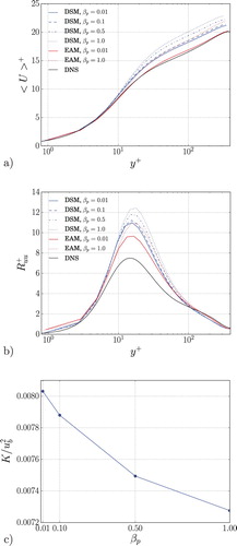
In an analogous way, the streamwise component of the Reynolds stress tensor (Figure 1(b)) shows the sensitivity of the fluctuating field to the different values of ${\text{β}}_p$. The influence of the R&C procedure is similar to the one denoted in the mean velocity profile: the inner layer peak amplitude exhibits a growing overestimation with an increasing ${\text{β}}_p$ coefficient. The volume-averaged total turbulent kinetic energy is plotted as a function of the ${\text{β}}_p$ coefficient (in Figure 1(c)). There a reduction of turbulent kinetic energy is visible when increasing the ${\text{β}}_p$ coefficient.

Additional results computed at the same friction Reynolds number with the EAM show essentially the same behaviour. In Figure 1(a,b) the use of a smaller ${\text{β}}_p$ leads to a more accurate prediction of the mean velocity profile and the streamwise Reynolds stress component, as compared to the case with ${\text{β}}_p=1.0$. Note that the use of EAM provides a further improvement to all the results shown.

Spanwise spectra show that the pressure fluctuations are evidently influenced by the R&C interpolation (Figure 2(a)). At low wavenumbers, a lower ${\text{β}}_p$ coefficient leads to a reduction of the pressure spectrum amplitude. This is partly due to the associated changes in skin friction, which is used for normalisation of $E_{pp}$. At high wavenumbers, the reduced R&C filter effect causes a pile-up of energy regardless of the choice of the model, although only by small amount.

Figure 2. Spanwise spectrum of (a) the pressure and (b) the velocity in inner units as a function of the spanwise wavelength, at the centreline. ${\mathrm{R}\mathrm{e}}_{\tau }\approx 550$ and resolution $(\mathrm{\Delta }{x}^{+},\mathrm{\Delta }{z}^{+})\approx (41,27)$. LES with EAM (red), LES with DSM (blue), LES with NM (green), $C{k}_z^{-7/3}$ law (black) in (a), $C{k}_z^{-5/3}$ law (black) in (b), cases ${\text{β}}_p=0.01$ in solid lines, ${\text{β}}_p=1.0$ in dashed lines.

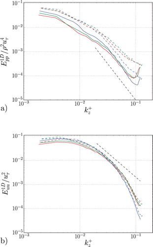
For all cases, the R&C interpolation will give an overprediction of pressure fluctuations since pressure spectra computed with ${\text{β}}_p=1.0$ lie above the cases with ${\text{β}}_p=0.01$.

In contrast, the behaviour of the velocity spectra (Figure 2(b)) is largely independent of the choice of the ${\text{β}}_p$ coefficient. However, LES with DSM shows a larger energy dissipation for the highest wavenumbers.

3.3. Simulations for two different ${\mathrm{R}\mathrm{e}}_{\tau }$

Once we established ${\text{β}}_p=0.01$ in order to minimise the R&C interpolation effect in LES, we carried out a set of LES with a larger computational domain, $4\pi \delta$ long and $2\pi \delta$ wide. Such domain has been chosen to allow the LES to capture the whole amount of kinetic energy needed for complete spectra, according to [38]. The friction Reynolds number cases investigated are ${\mathrm{R}\mathrm{e}}_{\tau }=550$ and 934. The numerical settings are equal to the previous ones. The bulk Reynolds number $u_b$ is used as input and is the same as that of the DNS from [39], 10,000 and 18,518, respectively.

Different grids are used, where the coarsest one has the following spacings in inner units $(\mathrm{\Delta }{x}^{+},\mathrm{\Delta }{z}^{+})\approx (165,108)$, and the finest $(\mathrm{\Delta }{x}^{+},\mathrm{\Delta }{z}^{+})\approx (41,27)$. The stretching ratio of the cells in the wall-normal direction is equal to the previous cases.

Different SGS models are employed, the Dynamic Smagorinsky model (DSM), consistent with the formulation in [21] and the Explicit Algebraic Model (EAM), as well as simulations with no-model (NM) (see Table 1).

Table 1. Channel flow simulations, from ${\mathrm{R}\mathrm{e}}_{\tau }\approx 550$ up to ${\mathrm{R}\mathrm{e}}_{\tau }\approx 934$. $N_x$, $N_y$, $N_z$ are the numbers of nodes in the streamwise, wall-normal and spanwise directions, respectively. $\mathrm{\Delta }{y}_w^{+}$ and $\mathrm{\Delta }{y}_c^{+}$ are the grid spacings in wall-normal direction at the wall and at the channel flow centreline. The label ‘B1’ denotes the cases where a ${\text{β}}_p=1.0$ setting has been used. DNS data by [39].

Case name	SGS model	$N_x\times N_y\times N_z$	$\mathrm{\Delta }{x}^{+}$	$\mathrm{\Delta }{z}^{+}$	$\mathrm{\Delta }{y}_w^{+}\sim \mathrm{\Delta }{y}_c^{+}$	${\mathrm{R}\mathrm{e}}_{\tau }$
DSM550VC	DSM	$42\times 84\times 32$	165	108	$0.95\sim 40$	399
EAM550VC	EAM	$42\times 84\times 32$	165	108	$0.95\sim 40$	419
NM550VC	NM	$42\times 84\times 32$	165	108	$0.95\sim 40$	404
DSM550C	DSM	$84\times 84\times 64$	82	54	$0.95\sim 40$	467
EAM550C	EAM	$84\times 84\times 64$	82	54	$0.95\sim 40$	491
NM550C	NM	$84\times 84\times 64$	82	54	$0.95\sim 40$	471
DSM550S	DSM	$116\times 84\times 86$	60	40	$0.95\sim 40$	492
EAM550S	EAM	$116\times 84\times 86$	60	40	$0.95\sim 40$	505
NM550S	NM	$116\times 84\times 86$	60	40	$0.95\sim 40$	496
DSM550F	DSM	$168\times 84\times 128$	41	27	$0.95\sim 40$	522
EAM550F	EAM	$168\times 84\times 128$	41	27	$0.95\sim 40$	543
NM550F	NM	$168\times 84\times 128$	41	27	$0.95\sim 40$	523
DSM550FB1	DSM	$168\times 84\times 128$	41	27	$0.95\sim 40$	481
EAM550FB1	EAM	$168\times 84\times 128$	41	27	$0.95\sim 40$	501
NM550FB1	NM	$168\times 84\times 128$	41	27	$0.95\sim 40$	482
DSM950VC	DSM	$72\times 144\times 55$	163	107	$0.94\sim 41$	703
EAM950VC	EAM	$72\times 144\times 55$	163	107	$0.94\sim 41$	728
NM950VC	NM	$72\times 144\times 55$	163	107	$0.94\sim 41$	708
DSM950C	DSM	$144\times 144\times 110$	82	53	$0.94\sim 41$	820
EAM950C	EAM	$144\times 144\times 110$	82	53	$0.94\sim 41$	851
NM950C	NM	$144\times 144\times 110$	82	53	$0.94\sim 41$	822
DSM950CB1	DSM	$144\times 144\times 110$	82	53	$0.94\sim 41$	756
EAM950CB1	EAM	$144\times 144\times 110$	82	53	$0.94\sim 41$	781
NM950CB1	NM	$144\times 144\times 110$	82	53	$0.94\sim 41$	751
DSM950S	DSM	$196\times 144\times 148$	60	40	$0.94\sim 41$	860
EAM950S	EAM	$196\times 144\times 148$	60	40	$0.94\sim 41$	893
NM950S	NM	$196\times 144\times 148$	60	40	$0.94\sim 41$	861
DSM950F	DSM	$288\times 144\times 220$	41	27	$0.94\sim 41$	901
EAM950F	EAM	$288\times 144\times 220$	41	27	$0.94\sim 41$	933
NM950F	NM	$288\times 144\times 220$	41	27	$0.94\sim 41$	904
DSM950FB1	DSM	$288\times 144\times 220$	41	27	$0.94\sim 41$	845
EAM950FB1	EAM	$288\times 144\times 220$	41	27	$0.94\sim 41$	861
NM950FB1	NM	$288\times 144\times 220$	41	27	$0.94\sim 41$	841
DNS550	DNS	$1024\times 257\times 1024$	13.4	6.7	$\mathrm{\Delta }{y}_{max}^{+}=6.7$	547
DNS934	DNS	$2048\times 385\times 1536$	11	5.7	$\mathrm{\Delta }{y}_{max}^{+}=N/A$	934

In a similar way of the low-dissipative solver tests, a fixed timestep that corresponds to a maximum Courant Number of 0.2 has been employed for the following simulations. However, in the coarse mesh cases (C) the maximum Courant Number constraint has been decreased to 0.1 to ensure a maximum viscous Courant Number limit to less than 1.

4. Improvement of the EAM

The estimation of the wall-normal Reynolds stress tensor component is important, especially for the prediction of flows in complex geometries. As an additional study, we have modified the formulation of the EAM in order to replace the limitation of ${\tau }_{22}$. The modification results from analysing the SGS anisotropy behaviour near the wall, and enforces strict realisability of the SGS stresses. The second component of the SGS anisotropy tensor reads (12) $a_{22}={\text{β}}_1{\tilde{S}}_{22}{\tau }^{\ast }+{\text{β}}_4\left({\tau }^{\ast }{)}^2\right({\tilde{S}}_{21}{\tilde{\mathrm{\Omega }}}_{12}-{\tilde{\mathrm{\Omega }}}_{21}{\tilde{S}}_{12})$(12) At the wall the first term on the r.h.s. can be neglected and the expression can be approximated by (13) $a_{22,w}\approx \frac{1}{2}{\text{β}}_{4,w}({\tau }_{+,w}^{\ast }{)}^2$(13) where the quantities with the subscript w are wall quantities, and ${\tau }_{+}^{\ast }$ is the SGS timescale in wall units. By noting that the values of $a_{22}$ and ${\tau }_{+}^{\ast }$ approach $-2/3$ and 2, respectively, at the wall, the minimum value of $c_1$ must be 0.43 for consistency (by use of Equation (6(6) ${\text{β}}_1=-\frac{33}{20}\frac{9c_1/4}{\left[\right(9c_1/4{)}^2+|{\tilde{\mathrm{\Omega }}}^{\ast }{|}^2]},{\text{β}}_4=-\frac{33}{20}\frac{1}{\left[\right(9c_1/4{)}^2+|{\tilde{\mathrm{\Omega }}}^{\ast }{|}^2]}$(6) )). The resulting value of $c_{min}$ can be obtained by plugging the value of $c_{1,min}=0.43$ into the left equation of expression (9(9) $c_1=c_1^{\prime }\sqrt{c_3^{\prime }}\frac{c^{1.25}}{(2C_s{)}^{2.5}},{\tau }^{\ast }=c_3^{\prime }\frac{1.5C_k^{1.5}\sqrt{c}}{2C_s}|\tilde{S}{|}^{-1}$(9) ). 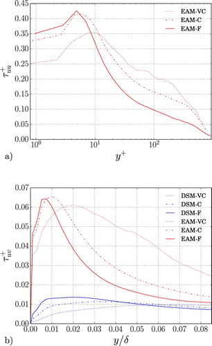We find $c_{min}=0.0085$, which is then used as an offset in the following way: (14) $c_1=c_1^{\prime }\sqrt{c_3^{\prime }}\frac{(c+c_{min}{)}^{1.25}}{(2C_s{)}^{2.5}}$(14) The new formulation enforces the correct behaviour of the SGS anisotropy near the wall, and is also coordinate-independent. This new improvement has been tested with the same settings as the case EAM550F.

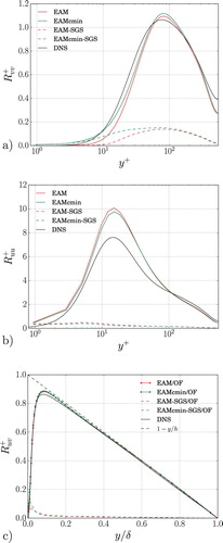
The sum of the resolved and SGS wall-normal Reynolds stress component is shown in Figure 3. LES with the new EAM (EAMcmin) shows a more physics-consistent behaviour of the SGS wall-normal Reynolds stress; the total wall-normal stress profile shifts towards the wall and gets closer to the DNS as compared to the LES with the classic EAM. All the other total Reynolds stress components are within 1–2% (see Figure 3(b,c)) compared to the original formulation of EAM. This is true also for the mean velocity profile. The results confirm that the new formulation of the EAM improves the near-wall behaviour.

Figure 3. (a) Wall-normal, (b) streamwise and (c) shear Reynolds stress tensor component as a function of the wall-normal direction in viscous units, for (a) ${\mathrm{R}\mathrm{e}}_{\tau }\approx 550$ with the same resolution as case F. Solid lines refer to the total spanwise Reynolds stress, while dashed lines to the SGS contribution.

5. Results

5.1. Skin friction coefficient

As a starting point, the predicted wall friction has been considered as a preliminary indicator of the LES accuracy, since the bulk Reynolds number is prescribed by the imposed mass flow. Figure 4(a) shows the values of the skin friction at the lowest Reynolds number, scaled with the DNS results, as a function of the streamwise resolution in wall units. Independently from the choice of the turbulence model, the predicted skin friction coefficient gets closer to the DNS values at high resolutions, showing a monotonic increasing behaviour. This is consistent with the results obtained by using a pseudo-spectral code [20], where similar skin friction coefficient ratios are achieved with resolutions in inner units that are two to three times larger compared to a finite-volume code ones, although with different cells' aspect ratios. The choice of the SGS model is essential for the prediction, and the use of the EAM helps to achieve a better estimation of the skin friction at any resolution, particularly when the resolution is the highest (case F). Here both the NM and DSM deviate from the DNS by about 10%, while the EAM results differ from the DNS by less than 2%. Results are similar when the Reynolds number is higher (see Figure 4(b)), although the results for all three alternatives are closer to the DNS than for the lower Reynolds number.

Figure 4. Skin friction coefficient ratio between LES and DNS as a function of the streamwise grid spacing in viscous units, for (a) ${\mathrm{R}\mathrm{e}}_{\tau }\approx 550$ and (b) ${\mathrm{R}\mathrm{e}}_{\tau }\approx 934$. Note that $\mathrm{\Delta }{z}^{+}\approx 0.66\mathrm{\Delta }{x}^{+}$.

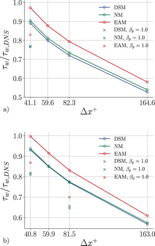
In agreement with [18], the skin friction ratio exhibits an overshoot at an even finer resolution. For the present study a resolution of $(\mathrm{\Delta }{x}^{+},\mathrm{\Delta }{z}^{+})\approx (30,18)$ at ${\mathrm{R}\mathrm{e}}_{\tau }\approx 550$ leads to a 6% overshoot, which is consistent with the study of Rasam, where a 7% overestimation was experienced with $(\mathrm{\Delta }{x}^{+},\mathrm{\Delta }{z}^{+})\approx (95,47)$. However, as confirmed by Rasam, yet finer grids yield results that approach the DNS value.

For the fine (case F) and coarse (C) (only for $R{e}_{\tau }\approx 934$) resolutions, we have included the skin friction coefficients computed when the R&C interpolation effect is maximum, with ${\text{β}}_p=1.0$ (i.e. the standard OpenFOAM setting). All the cases are strongly influenced by the R&C interpolation, and the skin friction discrepancy for DSM is almost 20% even at the fine resolution (case F), illustrating the deteriorating effect on the results from numerical dissipation in the standard OpenFOAM version.

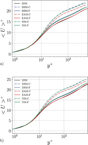
5.2. Mean velocity profiles

The log layer and the mean velocity up to the centreline is strongly influenced by the resolution and the SGS model (Figure 5). The coarsest resolution (case VC, not shown here) is not able to reasonably reproduce the correct physics although the results become slightly better with increasing Reynolds number. LES with DSM and NM give similar results with the differences becoming smaller at the higher Reynolds number. The EAM gives substantially improved predictions for both Reynolds numbers and all resolutions. At the fine resolution (case F) the mean velocity profile essentially collapses with the DNS results. The improvement with EAM over DSM can be translated to a reduction by about 50% in the number of grid points needed to achieve a given prediction accuracy.

Figure 5. Mean velocity profiles in inner units as a function of the wall-normal direction with different SGS models and grid resolutions, for (a) ${\mathrm{R}\mathrm{e}}_{\tau }\approx 550$ and (b) ${\mathrm{R}\mathrm{e}}_{\tau }\approx 934$.

5.3. Reynolds stresses

In the LES formulation, the total Reynolds stresses are the sum of the resolved part and the SGS part, i.e.: (15) $R_{ij}=⟨{\tilde{u}}_i{\tilde{u}}_j+{\tau }_{ij}⟩$(15) where $⟨.⟩$ is the averaging in time and in the homogeneous directions.

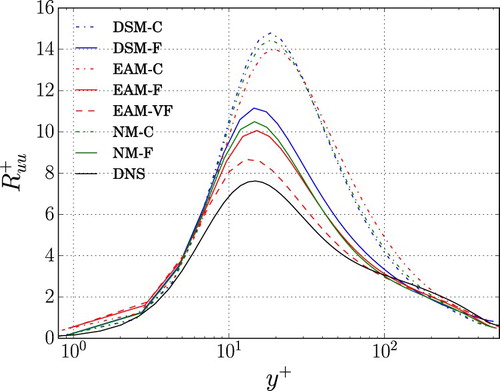
Similarly to the mean velocity, also the streamwise component of the Reynolds stress tensor (see Figure 6(a)) shows a grid independent region close to the wall for all the resolutions adopted. LES with the EAM is slightly closer to the DNS. Only the higher Reynolds number results are shown in Figure 6, but the results are similar for both. These results are in accordance with the results obtained with a pseudo-spectral code [20], although the EAM shows larger improvements when the pseudo-spectral code is used. These larger improvements are likely due to remaining levels of numerical dissipation in OpenFOAM which conceals the influence of the model. For both the grid C and F, LES with all the models give a trend that is mostly imposed by the resolution. However, LES with the EAM shows a slightly reduced overestimation of the inner layer peak, which is due to its ability of capturing SGS anisotropy. In contrast, the SGS contribution to the normal stresses for the DSM is unknown and therefore assumed to be zero. The magnitude of the SGS contribution from EAM decreases with increased resolution, which is consistent with the decreased filter width and a smaller contribution of the SGS turbulence. However, close to the wall there is an opposite trend of decreased SGS contribution with decreased resolution where the dynamic procedure actively is compensating for the lack of resolution in this area. Such behaviour is due to the low order of spatial discretisation, and has not been experienced in LES with a pseudo-spectral code [20].

Figure 6. (a) Streamwise and (b) shear component (SGS + resolved) of the Reynolds stress tensor in inner units as a function of the wall-normal direction with different SGS models and grid resolutions, for ${\mathrm{R}\mathrm{e}}_{\tau }\approx 934$.

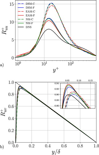
Note that the non-zero SGS stress at the wall is caused by the finite resolution. The use of a finer mesh would lead to a vanishing value at the wall.

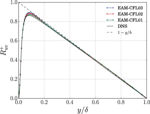
The shear stress profiles in Figure 6(b) show that all the simulations are statistically well converged and a clear distinction of the cases relative to the grid resolution used is noticeable, especially in proximity of the inner peak. The small magnitude of the mean spanwise velocity over the wall-normal direction compared to the bulk velocity ($|⟨W⟩{|}_{max}/U_b\sim \mathcal{O}\left({10}^{-4}\right)$) confirms the statistical convergence of the results. For a given resolution the predictions by the different models differ. Close to the wall the prediction of the peak position by LES with EAM is improved compared to the others. This is related to the role of the SGS part that adjusts to the degree of SGS anisotropy associated with a given resolution (see Figure 7(b)). Here the amplitude of the SGS part in the EAM is four times larger compared to that for DSM. A similar trend has been found in pseudo-spectral results [20], with larger magnitudes of the SGS stresses for both the LES with DSM and EAM. The high amount of numerical dissipation that is experienced in low-order finite-volume codes is most likely responsible for influencing the dynamic procedure in particular, resulting in substantially reduced SGS stress magnitudes compared to the pseudo-spectral results. The dependency on the grid resolution is analogous to what has been noticed for the streamwise component. All the total Reynolds shear stresses are affected by an overshoot compared to the DNS in proximity of the inner layer peak. The overshoot can be reduced by lowering the CFL number to 0.1, as described in Appendix 2.

Figure 7. Streamwise (a) and shear stress (b) SGS component of the Reynolds stress tensor in inner units as a function of the wall-normal direction with different SGS models and grid resolutions, for ${\mathrm{R}\mathrm{e}}_{\tau }\approx 934$.

The coarsest resolution (case VC, not shown here) gives a larger amplitude of the SGS contribution, especially far from the wall. For all the models the misprediction of the stresses, maximum towards the inner peak, is the largest, compared to finer resolutions. On the other hand, an additional simulation using the EAM at ${\mathrm{R}\mathrm{e}}_{\tau }\approx 550$ and a resolution of $(\mathrm{\Delta }{x}^{+},\mathrm{\Delta }{z}^{+})\approx (30,18)$ confirmed that the gap between LES with EAM and DNS is reduced for all the Reynolds stress components when a fine grid is adopted (see case EAM-VF in Figure 8).

Figure 8. Streamwise component (SGS + resolved) of the Reynolds stress tensor in inner units as a function of the wall-normal direction with different SGS models and grid resolutions, for ${\mathrm{R}\mathrm{e}}_{\tau }\approx 550$. The case EAM-VF refers to an LES with the EAM with $N_x\times N_y\times N_z=224\times 84\times 192$ and $(\mathrm{\Delta }{x}^{+},\mathrm{\Delta }{z}^{+})\approx (30,18)$.

5.4. Energy spectra

The prediction of the large-scale structures by LES with the EAM has been analysed by calculating the premultiplied spanwise energy spectra of the streamwise velocity as a function of the wall distance at ${\mathrm{R}\mathrm{e}}_{\tau }\approx 550$ and 934, defined as $k_z{\mathrm{\Phi }}_{uu}/u_{\tau }^2$, where $k_z$ is the spanwise wavenumber (Figure 9). At the lowest Reynolds number the position and wavenumber of the inner peak is close to the DNS. Moreover, the estimation of the peak position improves when the higher Reynolds number is considered, ${\mathrm{R}\mathrm{e}}_{\tau }\approx 934$. 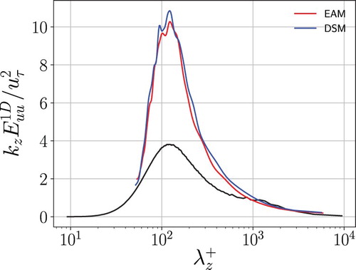Also the onset of the separation between the near-wall and the outer layer structures is captured by LES with the EAM. However, for both the Reynolds numbers, the number of grid points limits the accuracy of the spectra at small wavelengths. The prediction of the premultiplied spanwise energy spectra is similar for LES with DSM and EAM. However, LES with EAM gets a slightly better estimation of the spectra close to the wall (see Figure 10). There the energy in the LES with the DSM is slightly higher than in the LES with the EAM.

Figure 9. Premultiplied spanwise energy spectra of the streamwise velocity in inner units as a function of the spanwise wavelength and wall distance. DNS in the background, contours of LES with EAM for the fine resolution, for (a) ${\mathrm{R}\mathrm{e}}_{\tau }\approx 550$ and (b) ${\mathrm{R}\mathrm{e}}_{\tau }\approx 934$, with DNS at ${\mathrm{R}\mathrm{e}}_{\tau }\approx 1000$.

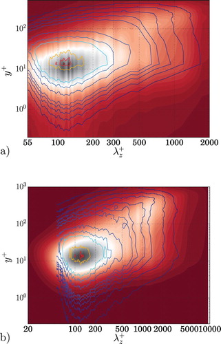
Figure 10. Premultiplied spanwise energy spectra of the streamwise velocity in inner units as a function of the spanwise wavelength at $y^{+}\approx 13$, for ${\mathrm{R}\mathrm{e}}_{\tau }\approx 934$.

6. Conclusion

The performance of the EAM has been analysed in LES of fully developed turbulent channel flow by using the general-purpose CFD code OpenFOAM. Two different Reynolds numbers are investigated at various resolutions. Results have been compared with LES with the DSM and LES without a model. DNS data is used as a reference. All the LESs are carried out using a novel numerical procedure to reduce the dissipation due to R&C interpolation, employed in the OpenFOAM pimpleFoam solver for incompressible flows. Tests with LES with the DSM showed that the excessive dissipative effects caused by R&C interpolation can be eliminated without numerical stability problems. Only a small pile-up of energy at the highest wavenumbers of the pressure spectrum was observed. It should be noted that this procedure so far has been tested only for fully developed turbulence on well-resolved regular meshes.

At the fine resolution (case F), which corresponds to a fairly typical resolution for wall-resolved LES, LES with the EAM gave a skin friction prediction within a few percent of the DNS value when the R&C interpolation influence was minimised. In contrast, LES with the DSM with standard setting, i.e. without reduced R&C filter activity, gave a skin friction prediction that deviated almost 20% from the DNS value.

The formulation of the EAM adds a non-linear term to the linear eddy-viscosity term, which improves the representation of the SGS stress anisotropy as compared to the commonly used eddy-viscosity based models (e.g. the DSM). Due to both the different dynamic procedure and the SGS anisotropy, the EAM SGS model was found to be more active with a different response for different resolutions in the near-wall and outer parts of the boundary layer. In LES with the DSM the SGS contribution was mostly small, irrespective of resolution, leading to results that were almost identical to LES without a model.

The use of EAM was shown to give substantial improvements for the prediction of the skin friction and the mean velocity profile. Some improvements were also found for other statistics such as the individual Reynolds stresses. The mean velocity prediction improvement can be translated to roughly a 50% reduction in the requirement for number of grid points to achieve a given degree of accuracy. Moreover, the model behaviour and grid dependency were found to be fairly consistent with previous results using a spectral discretisation. However, the resolution requirement is two to three times higher for this typical second-order finite volume method, compared to a spectral method.

In conclusion, it was shown that minimising numerical dissipation effects through reduced R&C filter activity in combination with the use of an anisotropy-capturing SGS model, the EAM, gave a substantial improvement of the LES prediction capability of OpenFOAM. These results can be transferred to other similar codes. For flows with laminar-turbulent interfaces special numerical treatments are likely needed.

Disclosure statement

No potential conflict of interest was reported by the authors.

ORCID

Matteo Montecchia  http://orcid.org/0000-0002-9645-5880

Additional information

Funding

Support from the Swedish Research Council [grant numbers 621-2014-5700 and 621-2016-03533] and computer time provided by the Swedish National Infrastructure for Computing (SNIC) are gratefully acknowledged.

Notes

1 In the present work orthogonal meshes are adopted, therefore the expression simplifies to ${\gamma }_f=|r_{j,N}-r_{j,f}|/|r_{j,N}-r_{j,P}|$.

Appendices

Appendix 1. EAM implementation

Part of the present work consisted in the implementation of the EAM in OpenFOAM v1712. The implementation of the model is strictly consistent to the description made in [19].

Let's now consider the momentum equation: (A1) $\frac{\mathrm{\partial }{\tilde{u}}_i}{\mathrm{\partial }t}+\frac{\mathrm{\partial }{\tilde{u}}_i{\tilde{u}}_j}{\mathrm{\partial }{x}_j}\underset{\begin{array}{c}-\mathrm{\partial }{T}_{ij}\end{array}/\mathrm{\partial }{x}_j}{\underbrace{-\frac{\mathrm{\partial }}{\mathrm{\partial }{x}_j}\left[\nu \left(\frac{\mathrm{\partial }{\tilde{u}}_i}{\mathrm{\partial }{x}_j}+\frac{\mathrm{\partial }{\tilde{u}}_j}{\mathrm{\partial }{x}_i}-\frac{2}{3}\frac{\mathrm{\partial }{\tilde{u}}_k}{\mathrm{\partial }{x}_k}{\delta }_{ij}\right)\right]+\frac{\mathrm{\partial }{\tau }_{ij}}{\mathrm{\partial }{x}_j}}}=-\frac{1}{\rho }\frac{\mathrm{\partial }\tilde{p}}{\mathrm{\partial }{x}_i}$(A1) where $\mathrm{\partial }{T}_{ij}/\mathrm{\partial }{x}_j$ is the divergence of the total stress. The divergence of the total stress has been implemented in the following form: (A2) $\begin{array}{rl}& -\frac{\mathrm{\partial }{T}_{ij}}{\mathrm{\partial }{x}_j}\stackrel{discr.}{=}{\mathrm{\nabla }}_j\left({\tau }_{ij}\right){|}_{\mathrm{e}\mathrm{x}\mathrm{p}}+\mathrm{\Delta }({\nu }_{\mathrm{S}\mathrm{G}\mathrm{S}},{\tilde{u}}_i){|}_{\mathrm{e}\mathrm{x}\mathrm{p}}-\mathrm{\Delta }(\nu +{\nu }_{\mathrm{S}\mathrm{G}\mathrm{S}},{\tilde{u}}_i){|}_{\mathrm{i}\mathrm{m}\mathrm{p}}\\ & {\left.-{\mathrm{\nabla }}_j\left[\nu \left(\frac{\mathrm{\partial }{\tilde{u}}_j}{\mathrm{\partial }{x}_i}-\frac{2}{3}\frac{\mathrm{\partial }{\tilde{u}}_k}{\mathrm{\partial }{x}_k}{\delta }_{ij}\right)\right]\right|}_{\mathrm{e}\mathrm{x}\mathrm{p}}\end{array}$(A2) where the subscripts $\mathrm{e}\mathrm{x}\mathrm{p}$ and $\mathrm{i}\mathrm{m}\mathrm{p}$ indicate an explicit and implicit discretisation, respectively. The terms ${\mathrm{\nabla }}_j$ and $\mathrm{\Delta }(\alpha ,q)$ are the discretised divergence and compact laplacian operators, respectively, such that $\frac{\mathrm{\partial }}{\mathrm{\partial }{x}_j}\stackrel{discr.}{=}{\mathrm{\nabla }}_j,\frac{\mathrm{\partial }}{\mathrm{\partial }{x}_j}\left(\alpha \frac{\mathrm{\partial }q}{\mathrm{\partial }{x}_j}\right)\stackrel{discr.}{=}\mathrm{\Delta }(\alpha ,q)$ where the coefficient α can vary in space. The SGS eddy-viscosity is described as ${\nu }_{\mathrm{S}\mathrm{G}\mathrm{S}}=-\frac{1}{2}{\text{β}}_1{K}^{\mathrm{S}\mathrm{G}\mathrm{S}}{\tau }^{\ast }$ which comes from the eddy-viscosity contribution of the EAM formulation.

A particular emphasis must be given on the two different discretisation schemes used for the laplacian. Let's consider a typical diffusion term of a quantity q with diffusivity α: $D=\frac{\mathrm{\partial }}{\mathrm{\partial }{x}_j}\left(\alpha \frac{\mathrm{\partial }q}{\mathrm{\partial }{x}_j}\right)$ This term can be discretised in two different ways using the discrete operators above, namely as $D_{\mathrm{L}}=\mathrm{\Delta }(\alpha ,q)\mathrm{o}\mathrm{r}{D}_{\mathrm{D}\mathrm{G}}={\mathrm{\nabla }}_j\left(\alpha {\mathrm{\nabla }}_j\right(q\left)\right)$$D_{\mathrm{L}}$ and $D_{\mathrm{D}\mathrm{G}}$ are mathematically identical, but the discrete representations are different. The Laplacian operator can be evaluated in one step using a compact stencil. The representation by the divergence-gradient, $D_{\mathrm{D}\mathrm{G}}$, would require two steps, first by computing the gradient and then to take the divergence, where each step also requires additional interpolation between cell faces and centres. Hence, the resulting stencil for $D_{\mathrm{D}\mathrm{G}}$ is much wider and would result in significant differences when discretising a typical LES field with poorly resolved fluctuations. The details of the discretisation in OpenFOAM will be given below, but the principle is similar for all finite volume or finite difference methods.

The total stress given above contains both terms that can be formulated as the compact Laplacian (e.g. $\mathrm{\partial }\left({\nu }_{\mathrm{S}\mathrm{G}\mathrm{S}}\mathrm{\partial }{\tilde{u}}_i/\mathrm{\partial }{x}_j\right)/\mathrm{\partial }{x}_j$) and terms that must be written in terms of the divergence of velocity gradients e.g. $\mathrm{\partial }{\tau }_{ij}/\mathrm{\partial }{x}_j$ where ${\tau }_{ij}$ also contains the transpose of the velocity gradients as well as higher order terms and non-constant scalars. It is necessary to use the same kind of discretisation for all the different terms for consistency and accuracy, hence the total stress term, the first term in Equation (A2(A2) $\begin{array}{rl}& -\frac{\mathrm{\partial }{T}_{ij}}{\mathrm{\partial }{x}_j}\stackrel{discr.}{=}{\mathrm{\nabla }}_j\left({\tau }_{ij}\right){|}_{\mathrm{e}\mathrm{x}\mathrm{p}}+\mathrm{\Delta }({\nu }_{\mathrm{S}\mathrm{G}\mathrm{S}},{\tilde{u}}_i){|}_{\mathrm{e}\mathrm{x}\mathrm{p}}-\mathrm{\Delta }(\nu +{\nu }_{\mathrm{S}\mathrm{G}\mathrm{S}},{\tilde{u}}_i){|}_{\mathrm{i}\mathrm{m}\mathrm{p}}\\ & {\left.-{\mathrm{\nabla }}_j\left[\nu \left(\frac{\mathrm{\partial }{\tilde{u}}_j}{\mathrm{\partial }{x}_i}-\frac{2}{3}\frac{\mathrm{\partial }{\tilde{u}}_k}{\mathrm{\partial }{x}_k}{\delta }_{ij}\right)\right]\right|}_{\mathrm{e}\mathrm{x}\mathrm{p}}\end{array}$(A2) ), must be discretised by the divergence of gradient approach even though it would result in an unnecessarily wider stencil for some of the terms.

The compact Laplacian term is well suited for implicit treatment contributing to the numerical stability. The principal stress term is therefore formulated as a compact Laplacian in terms of an effective viscosity $(\nu +{\nu }_{\mathrm{S}\mathrm{G}\mathrm{S}})$ and treated implicitly, the third term in (A2(A2) $\begin{array}{rl}& -\frac{\mathrm{\partial }{T}_{ij}}{\mathrm{\partial }{x}_j}\stackrel{discr.}{=}{\mathrm{\nabla }}_j\left({\tau }_{ij}\right){|}_{\mathrm{e}\mathrm{x}\mathrm{p}}+\mathrm{\Delta }({\nu }_{\mathrm{S}\mathrm{G}\mathrm{S}},{\tilde{u}}_i){|}_{\mathrm{e}\mathrm{x}\mathrm{p}}-\mathrm{\Delta }(\nu +{\nu }_{\mathrm{S}\mathrm{G}\mathrm{S}},{\tilde{u}}_i){|}_{\mathrm{i}\mathrm{m}\mathrm{p}}\\ & {\left.-{\mathrm{\nabla }}_j\left[\nu \left(\frac{\mathrm{\partial }{\tilde{u}}_j}{\mathrm{\partial }{x}_i}-\frac{2}{3}\frac{\mathrm{\partial }{\tilde{u}}_k}{\mathrm{\partial }{x}_k}{\delta }_{ij}\right)\right]\right|}_{\mathrm{e}\mathrm{x}\mathrm{p}}\end{array}$(A2) ). Since the SGS viscosity is already contained in the SGS stress a corresponding explicit term must be subtracted, the second term in (A2(A2) $\begin{array}{rl}& -\frac{\mathrm{\partial }{T}_{ij}}{\mathrm{\partial }{x}_j}\stackrel{discr.}{=}{\mathrm{\nabla }}_j\left({\tau }_{ij}\right){|}_{\mathrm{e}\mathrm{x}\mathrm{p}}+\mathrm{\Delta }({\nu }_{\mathrm{S}\mathrm{G}\mathrm{S}},{\tilde{u}}_i){|}_{\mathrm{e}\mathrm{x}\mathrm{p}}-\mathrm{\Delta }(\nu +{\nu }_{\mathrm{S}\mathrm{G}\mathrm{S}},{\tilde{u}}_i){|}_{\mathrm{i}\mathrm{m}\mathrm{p}}\\ & {\left.-{\mathrm{\nabla }}_j\left[\nu \left(\frac{\mathrm{\partial }{\tilde{u}}_j}{\mathrm{\partial }{x}_i}-\frac{2}{3}\frac{\mathrm{\partial }{\tilde{u}}_k}{\mathrm{\partial }{x}_k}{\delta }_{ij}\right)\right]\right|}_{\mathrm{e}\mathrm{x}\mathrm{p}}\end{array}$(A2) ). The viscous stress term can be represented completely by the Laplacian term since the last term in (A2(A2) $\begin{array}{rl}& -\frac{\mathrm{\partial }{T}_{ij}}{\mathrm{\partial }{x}_j}\stackrel{discr.}{=}{\mathrm{\nabla }}_j\left({\tau }_{ij}\right){|}_{\mathrm{e}\mathrm{x}\mathrm{p}}+\mathrm{\Delta }({\nu }_{\mathrm{S}\mathrm{G}\mathrm{S}},{\tilde{u}}_i){|}_{\mathrm{e}\mathrm{x}\mathrm{p}}-\mathrm{\Delta }(\nu +{\nu }_{\mathrm{S}\mathrm{G}\mathrm{S}},{\tilde{u}}_i){|}_{\mathrm{i}\mathrm{m}\mathrm{p}}\\ & {\left.-{\mathrm{\nabla }}_j\left[\nu \left(\frac{\mathrm{\partial }{\tilde{u}}_j}{\mathrm{\partial }{x}_i}-\frac{2}{3}\frac{\mathrm{\partial }{\tilde{u}}_k}{\mathrm{\partial }{x}_k}{\delta }_{ij}\right)\right]\right|}_{\mathrm{e}\mathrm{x}\mathrm{p}}\end{array}$(A2) ) will vanish for converged incompressible flows with constant viscosity.

The gradient operator of a cell-centred quantity ${\mathrm{\nabla }}_j\left(q\right)$ is defined as follows: (A3) $\mathcal{V}{\mathrm{\nabla }}_j\left(q\right)={\int }_{\mathcal{V}}\frac{\mathrm{\partial }q}{\mathrm{\partial }{x}_j}\mathrm{d}\mathcal{V}={\oint }_{\mathcal{S}}q{\hat{n}}_j\mathrm{d}\mathcal{S}\approx \sum _{\mathrm{f}\mathrm{a}\mathrm{c}\mathrm{e}\mathrm{s}}{q}_f\mathrm{\Delta }{\mathcal{S}}_{j,f}$(A3) where $\mathcal{V}$ is the cell volume, $q_f\approx {⟨q⟩}_f=q_P{\gamma }_f+(1-{\gamma }_f)q_N$ is the cell face average between the neighbouring N and present cell P, and $\mathrm{\Delta }{\mathcal{S}}_{j,f}$ is the cell face vector. ${\gamma }_f=|r_{j,N}-r_{j,f}|/|r_{j,N}-r_{j,P}|$ is the interpolation weight for interpolating the cell centre quantities to the face.

The next step for deriving the $D_{\mathrm{D}\mathrm{G}}={\mathrm{\nabla }}_j\left(\alpha {\mathrm{\nabla }}_j\right(q\left)\right)$ term is to take the divergence of the gradient $g_j={\mathrm{\nabla }}_j\left(q\right)$, where ${\mathrm{\nabla }}_j\left(q\right)$ is derived and described above. (A4) $\mathcal{V}{D}_{\mathrm{D}\mathrm{G}}=\mathcal{V}{\mathrm{\nabla }}_j\left(\alpha g_j\right)={\int }_{\mathcal{V}}\alpha \frac{\mathrm{\partial }{g}_j}{\mathrm{\partial }{x}_j}\mathrm{d}\mathcal{V}={\oint }_{\mathcal{S}}\alpha g_j{\hat{n}}_j\mathrm{d}\mathcal{S}\approx \sum _{\mathrm{f}\mathrm{a}\mathrm{c}\mathrm{e}\mathrm{s}}{\alpha }_f{g}_{j,f}\mathrm{\Delta }{\mathcal{S}}_{j,f}$(A4) where $g_{j,f}={\gamma }_P{g}_{j,P}+{\gamma }_N{g}_{j,N}$ is the cell face average of the vector $g_j$. Also ${\alpha }_f$ is the cell face average. The divergence-gradient of the velocity, e.g. for the $\mathrm{\partial }\left({\nu }_{\mathrm{S}\mathrm{G}\mathrm{S}}\mathrm{\partial }{\tilde{u}}_i/\mathrm{\partial }{x}_j\right)/\mathrm{\partial }{x}_j$ term, is made by applying the scheme for each component of the vector.

Computing the same term by the use of the Laplacian operator, $D_{\mathrm{L}}=\mathrm{\Delta }(\alpha ,q)$, is described in the following. Here, the Laplacian is directly discretised as (A5) $\mathcal{V}{D}_{\mathrm{L}}=\mathcal{V}{\mathrm{\nabla }}_j\left(\alpha g_j\right)={\int }_{\mathcal{V}}\alpha \frac{\mathrm{\partial }{g}_j}{\mathrm{\partial }{x}_j}\mathrm{d}\mathcal{V}={\oint }_{\mathcal{S}}\alpha g_j{\hat{n}}_j\mathrm{d}\mathcal{S}\approx \sum _{\mathrm{f}\mathrm{a}\mathrm{c}\mathrm{e}\mathrm{s}}{\alpha }_f{g}_{j,f}\mathrm{\Delta }{\mathcal{S}}_{j,f}$(A5) which is, so far, the same as Equation (A4(A4) $\mathcal{V}{D}_{\mathrm{D}\mathrm{G}}=\mathcal{V}{\mathrm{\nabla }}_j\left(\alpha g_j\right)={\int }_{\mathcal{V}}\alpha \frac{\mathrm{\partial }{g}_j}{\mathrm{\partial }{x}_j}\mathrm{d}\mathcal{V}={\oint }_{\mathcal{S}}\alpha g_j{\hat{n}}_j\mathrm{d}\mathcal{S}\approx \sum _{\mathrm{f}\mathrm{a}\mathrm{c}\mathrm{e}\mathrm{s}}{\alpha }_f{g}_{j,f}\mathrm{\Delta }{\mathcal{S}}_{j,f}$(A4) ). The gradient at the cell face, $g_{j,f}$, can be decomposed into two parts, $g_{j,f}=g_{j,f}^{\perp }+g_{j,f}^{\parallel }$, where $g_{j,f}^{\perp }$ and $g_{j,f}^{\parallel }$ are the gradient normal and tangential to the cell face respectively. $g_{j,f}^{\perp }$ is simply derived by taking the difference between the cell-centred values: $g_{j,f}^{\perp }=\frac{q_N-q_P}{|d_j|}{\hat{d}}_j$ where $d_j$ is the length vector between the centre of the cell of interest P and the centre of a neighbouring cell N. The tangential component of the gradient instead is $g_{j,f}^{\parallel }={\gamma }_P{g}_{j,P}+{\gamma }_N{g}_{j,N}-\left[\right({\gamma }_P{g}_{k,P}+{\gamma }_N{g}_{k,N}\left){\hat{d}}_k\right]{\hat{d}}_j$ The gradients $g_{j,N}$ and $g_{j,P}$, are derived by using the gradient operator in (A3(A3) $\mathcal{V}{\mathrm{\nabla }}_j\left(q\right)={\int }_{\mathcal{V}}\frac{\mathrm{\partial }q}{\mathrm{\partial }{x}_j}\mathrm{d}\mathcal{V}={\oint }_{\mathcal{S}}q{\hat{n}}_j\mathrm{d}\mathcal{S}\approx \sum _{\mathrm{f}\mathrm{a}\mathrm{c}\mathrm{e}\mathrm{s}}{q}_f\mathrm{\Delta }{\mathcal{S}}_{j,f}$(A3) ). The tangential component of the face gradient would, hence, need a wider stencil than the normal component. For an orthogonal mesh $g_{j,f}^{\parallel }{\hat{n}}_j=0$, so the expression (A5(A5) $\mathcal{V}{D}_{\mathrm{L}}=\mathcal{V}{\mathrm{\nabla }}_j\left(\alpha g_j\right)={\int }_{\mathcal{V}}\alpha \frac{\mathrm{\partial }{g}_j}{\mathrm{\partial }{x}_j}\mathrm{d}\mathcal{V}={\oint }_{\mathcal{S}}\alpha g_j{\hat{n}}_j\mathrm{d}\mathcal{S}\approx \sum _{\mathrm{f}\mathrm{a}\mathrm{c}\mathrm{e}\mathrm{s}}{\alpha }_f{g}_{j,f}\mathrm{\Delta }{\mathcal{S}}_{j,f}$(A5) ) results in (A6) $\mathcal{V}{D}_{\mathrm{L}}\approx \sum _{\mathrm{f}\mathrm{a}\mathrm{c}\mathrm{e}\mathrm{s}}{\alpha }_f{g}_{j,f}\mathrm{\Delta }{\mathcal{S}}_{j,f}=\sum _{\mathrm{f}\mathrm{a}\mathrm{c}\mathrm{e}\mathrm{s}}{\alpha }_f\frac{q_N-q_P}{|d_j|}{\hat{d}}_j\mathrm{\Delta }{\mathcal{S}}_{j,f}$(A6) Orthogonality here means that the surface normal is in the direction of the neighbouring cell centres. Hence, also a triangular unstructured mesh can be orthogonal. Moreover, near-orthogonal mesh will have the dominating contribution from the compact normal contribution to the face gradient resulting in only a small contribution from the wider discretisation stencil.

Appendix 2. CFL number influence in OpenFOAM

The influence of the CFL number has been investigated by performing the previously described case EAM550F with the CFL numbers of 0.1, 0.2 and 0.3 using the same resolutions listed in Table 1. As shown in Figure A1, the mean velocity profile and the streamwise component of the Reynolds stress tensor are essentially independent of the CFL number. By contrast, the peaks of the wall-normal and shear components are influenced by the time discretisation. The peak value of the shear stress decreases if the CFL number decreases and comes closer to the DNS data.

Figure A.1. (a) Mean velocity profile, (b) streamwise and (c) wall-normal Reynolds stress components in wall units as a function of the inner-scaled wall-normal direction for $R{e}_{\tau }\approx 550$.

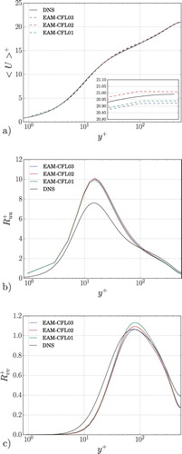
Figure A.2. Reynolds shear stress component in wall units as a function of the inner-scaled wall-normal direction for ${\mathrm{R}\mathrm{e}}_{\tau }\approx 550$, case EAM550F.

References

- Tucker PG, Lardeau S. Applied large eddy simulation. Phil Trans R Soc A. 2009;367:2809–2818.
- Bouffanais R. Advances and challenges of applied large-eddy simulation. Comput Fluids. 2010;39(5):735–738.
- Georgiadis NJ, Rizzetta DP, Fureby C. Large-eddy simulation: current capabilities, recommended practices, and future research. AIAA J. 2010;48(8):1772–1784.
- Seung JK, Hyung JS, Wallin S, et al. Design of the centrifugal fan of a belt-driven starter generator with reduced flow noise. Int J Heat Fluid Flow. 2019;76:72–84.
- Tabib M, Rasheed A, Kvamsdal T. LES and RANS simulation of onshore bessaker wind farm: analysing terrain and wake effects on wind farm performance. J Phys: Conf Ser. 2015;625:012032.
- Javadi A, Nilsson H. LES and DES of strongly swirling turbulent flow through a suddenly expanding circular pipe. Comput Fluids. 2015;107:301–313.
- Piomelli U. Large-eddy simulation: achievements and challenges. Prog Aerosp Sci. 1999;35(4):335–362.
- Breuer M. Large eddy simulation of the subcritical flow past a circular cylinder: numerical and modeling aspects. Int J Numer Meth Fl. 1998;28(9):1281–1302.
- Kawai S, Larsson J. Wall-modeling in large eddy simulation: length scales, grid resolution, and accuracy. Phys Fluids. 2012;24(1):015105.
- Spalart PR. Detached-eddy simulation. Ann Rev Fluid Mech. 2009;41:181–202.
- Rezaeiravesh S, Liefvendahl M. Effect of grid resolution on large eddy simulation of wall-bounded turbulence. Phys Fluids. 2018;30(5):055106.
- Mukha T. Modelling techniques for large-eddy simulation of wall-bounded turbulent flows [dissertation]. Uppsala University; 2018.
- Vuorinen V, Keskinen JP, Duwig C, et al. On the implementation of low-dissipative Runge–Kutta projection methods for time dependent flows using OpenFOAM. Comput Fluids. 2014;93:153–163.
- Breuer M. Numerical and modeling influences on large eddy simulations for the flow past a circular cylinder. Int J Heat Fluid Flow. 1998;19(5):512–521.
- Silvis MH, Remmerswaal RA, Verstappen R. Physical consistency of subgrid-scale models for large-eddy simulation of incompressible turbulent flows. Phys Fluids. 2017;29(1):015105.
- Piomelli U, Rouhi A, Geurts BJ. A grid-independent length scale for large-eddy simulations. J Fluid Mech. 2015;766:499–527.
- Rouhi A, Piomelli U, Geurts BJ. Dynamic subfilter-scale stress model for large-eddy simulations. Phys Rev Fluids. 2016;1(4):044401.
- Rasam A, Brethouwer G, Schlatter P, et al. Effects of modelling, resolution and anisotropy of subgrid-scales on large eddy simulations of channel flow. J Turbul. 2011;12.
- Marstorp L, Brethouwer G, Grundestam O, et al. Explicit algebraic subgrid stress models with application to rotating channel flow. J Fluid Mech. 2009;639:403–432.
- Montecchia M, Brethouwer G, Johansson AV, et al. Taking large-eddy simulation of wall-bounded flows to higher Reynolds numbers by use of anisotropy-resolving subgrid models. Phys Rev Fluids. 2017;2(3):034601.
- Germano M, Piomelli U, Moin P, et al. A dynamic subgrid-scale eddy viscosity model. Phys Fluids A. 1991;3(7):1760–1765.
- Lilly DK. A proposed modification of the germano subgrid-scale closure method. Phys Fluids A. 1992;4(3):633–635.
- Rasam A, Wallin S, Brethouwer G, et al. Large eddy simulation of channel flow with and without periodic constrictions using the explicit algebraic subgrid-scale model. J Turbul. 2014;15(11):752–775.
- Lee M, Moser RD. Direct numerical simulation of turbulent channel flow up to Reτ≈5200. J Fluid Mech. 2015 Jul;774:395–415.
- Cadieux F, Sun G, Domaradzki JA. Effects of numerical dissipation on the interpretation of simulation results in computational fluid dynamics. Comput Fluids. 2017;154:256–272.
- Wallin S, Johansson AV. An explicit algebraic Reynolds stress model for incompressible and compressible turbulent flows. J Fluid Mech. 2000;403:89–132.
- Yoshizawa A. Statistical theory for compressible turbulent shear flows, with the application to subgrid modeling. Phys Fluids. 1986;29(7):2152–2164.
- Montecchia M, Knacke T, Brethouwer G, et al. Improved LES of turbulent channel flow by using OpenFOAM with the Explicit Algebraic SGS model. 12th International ERCOFTAC Symposium on Engineering Turbulence Modelling and Measurements; 2018.
- Holzmann T. Mathematics, numerics, derivations and openfoam(r). Holzmann CFD; 2018.
- Ferziger JH, Perić M. Computational methods for fluid dynamics. 3rd ed: Berlin: Springer; 2002.
- Knacke T. Potential effects of Rhie & Chow type interpolations in airframe noise simulations. In: Schram C, Dénos R, Lecomte E, editors. Accurate and efficient aeroacoustic prediction approaches for airframe noise. Rhode-Saint-Genèse: Von Kármán Institute for Fluid Dynamics; 2013. (VKI lecture notes).
- Knacke T. Numerische Simulation des Geräusches massiv abgelöster Strömung bei großer Reynoldszahl und kleiner Machzahl [Numerical simulation of noise from flows with massive separation at large Reynolds number and small mach number] [dissertation]. Technische Universität Berlin; 2015.
- Johansson P, Davidson L. Modified collocated SIMPLEC algorithm applied to a buoyancy-affected turbulent flow using a multigrid solution procedure. Numer Heat Tr B-Fund. 1995;28(1):39–57.
- Pascau A. Cell face velocity alternatives in a structured colocated grid for the unsteady Navier–Stokes equations. Int J Numer Meth Fluids. 2009. Available from: https://doi.org/10.1002/fld.2215
- Cubero A, Fueyo N. A compact momentum interpolation procedure for unsteady flows and relaxation. Numer Heat Tr B. 2007;52:507–529.
- Moser RD, Kim J, Mansour NN. Direct numerical simulation of turbulent channel flow up to Reτ=590. Phys Fluids. 1999;11(4):943–945.
- Schoppa W, Hussain F. Coherent structure dynamics in near-wall turbulence. Fluid Dyn Res. 2000;26(2):119.
- Lozano-Durán A, Jiménez J. Effect of the computational domain on direct simulations of turbulent channels up to re τ=4200. Phys Fluids. 2014;26(1):011702.
- Hoyas S, Jiménez J. Reynolds number effects on the Reynolds-stress budgets in turbulent channels. Phys Fluids. 2008;20(10):101511.