Honeycomb-generated Reynolds-number-dependent wake turbulence

ABSTRACT

We present an experimental and numerical study of the flow downstream of honeycomb flow straighteners for a range of Reynolds numbers, covering both laminar and turbulent flow inside the honeycomb cells. We carried out experiments with planar particle image velocimetry (PIV) in a wind tunnel and performed numerical simulations to perform an in-depth investigation of the three-dimensional flow field. The individual channel profiles downstream of the honeycomb gradually develop into one uniform velocity profile. This development corresponds with an increase in the velocity fluctuations which reach a maximum and then start to decay. The position and magnitude of the turbulence intensity peak depend on the Reynolds number. By means of the turbulence kinetic energy (TKE) budget it is shown that the production of TKE is dominated by the shear layers corresponding to the honeycomb walls. The near-field and far-field decay of the turbulence intensity can be described by power laws where we used the position where the production term of the TKE reaches its maximum as the virtual origin.

KEYWORDS:

• Honeycomb
• wake turbulence
• turbulence kinetic energy budget
• turbulence decay power law

1. Introduction

Flow straighteners have often been used to reduce the turbulence level in wind- and water tunnels. An example of a flow straightener is a honeycomb which consists of many parallel channels with square, circular or regular hexagonal cross-sections. An example of the usage of honeycombs in an industrial system where the turbulence level must be as low as possible is the magnetic density separation machine [1–3].

Magnetic density separation (MDS) is a promising recycling technique that can improve the sustainable usage of plastic [4]. A schematic representation of the MDS setup is shown in Figure 1. The MDS technique uses a magnetic field applied to a ferrofluid to generate a specific effective mass density gradient in the fluid. This ferrofluid flows through a flow laminator, or honeycomb, before it enters the separation chamber. The honeycomb is used to suppress the turbulence level in the flow such that the flow has as little disturbance as possible. To this end, conveyor belts are installed on the top and bottom of the channel and move with the mean streamwise velocity. The conveyor belts are installed to prevent the formation of boundary layers. Shredded plastic waste, which is a collection of various types of plastics, is injected on the left top and bottom and will settle to its equilibrium height in the separation chamber according to its mass density. The plastic particles will be separated by separator blades further downstream and are ready for post-processing, for example separation on colour. The characteristics of the flow inside the MDS machine are of key importance to obtain a good separation efficiency. The main challenge is to obtain a flow in the separation chamber which has as little disturbance as possible, while maintaining a high velocity to obtain a large throughput. Therefore, this research focuses on the flow in the wake of the honeycomb for a range of velocities close to the critical Reynoldsnumber.

Figure 1. A schematic representation of the magnetic density separation setup. Different markers (colours) represent plastic particles with different mass densities [1].

Lumley et al. [5,6] investigated the passage of turbulent flow through a honeycomb by means of hot-film probe experiments in a water tunnel. They concluded that the suppression of turbulence is mostly dominated by the inhibition of the lateral components of the velocity fluctuations. The flow that leaves the honeycomb is not always laminar, as small turbulent eddies with a length scale smaller than the cell diameter will remain in the flow. Using a honeycomb with a smaller cell diameter enhances the suppression of these turbulent eddies. However, too small cells have practical disadvantages like blockage of the flow and a larger pressure loss.

Loehrke and Nagib [7] visualised the flow downstream of a honeycomb and measured the velocity with a hot-wire anemometer. The honeycomb was located in a compressed-air driven wind tunnel and consisted of a bundle of plastic drinking straws with an inner diameter of 0.455 cm and a length of 2.5, 7.5, or 25 cm. They showed that honeycombs suppress turbulence, but further downstream additional turbulence is created due to shear layer instabilities. Both Lumley et al. [5,6] and Loehrke and Nagib [7] explained that the additional turbulence is generated via the break-up of the mean velocity profile from each cell.

Farell and Youssef [8] performed similar experiments as Loehrke and Nagib [7]. They measured the mean and rms velocity with hot-wire anemometer technique. They used a bundle of plastic drinking straws with an inner diameter of 5.95 mm and a length of 50.8, 127, or 254 mm. They showed that by using honeycombs the turbulence intensity was reduced by a factor 1.7.

Mikhailova et al. [9] showed that with an increasing free stream velocity the turbulence intensity peak shifts further upstream. Furthermore, they showed that increasing the turbulence level of the free stream leads to an upstream displacement of the transition zone.

Xiong et al. [10] and Kühnen et al. [11] both performed experiments with particle image velocimetry (PIV). Xiong et al. [10] used two perforated plates and a tube bundle. They stated that the honeycomb induced flow instabilities disappear at the end of the near field and the decay of the disturbance caused by the installation takes place in the far-field. Kühnen et al. [11] used 3D printed honeycombs and determined the pressure drop over the honeycomb.

Numerical simulations were performed by Kulkarni et al. [12]. They used ANSYS-CFX to investigate the effectiveness of honeycombs with different lengths and different cell shapes for the reduction of turbulence. They also considered combinations of honeycombs with screens. Their model predicts a turbulence reduction factor which is optimal for a length-to-diameter ratio between 8 and 10.

Although many studies on the effects of honeycombs have been performed, there are no studies on the dependency of the turbulence intensity in a range of cell Reynolds numbers close to the critical Reynolds number, on the terms in the turbulence kinetic energy (TKE) budget downstream of the honeycomb, and on the decay of the turbulence in laminar and turbulent conditions. These properties are relevant for the design of the honeycomb used in MDS and in other applications where a honeycomb is applied to relaminarise a flow. In this paper, we present the results of an investigation on the flow field downstream of a honeycomb for a range of cell Reynolds numbers around the critical Reynolds number. We carried out experiments with planar particle image velocimetry (PIV) in a wind tunnel and performed direct numerical simulations for an in-depth investigation of the three-dimensional flow field.

The paper is organised as follows. Section 2 describes the honeycomb dimensions, the experimental set-up, and the numerical model. Section 3 presents the results, where first the turbulence intensity results are provided, the terms in the TKE budget are analysed and then the turbulence decay power law is derived. The experimental results serve to validate the numerical method, which is applied to compute all terms in the TKE budget equation. Finally, conclusions are provided in Section 4.

2. Methods

In this section, we present the methods used to analyse the flow downstream of a honeycomb. First, more details are given about the honeycomb and its dimensions. The flow is analysed using both an experimental and a numerical approach.

2.1. Honeycomb structure

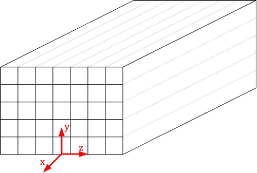
Figure 2 shows the schematic of the honeycomb used in this research. For the experimental set-up a 3D printed honeycomb is used. The honeycomb is produced with SLA stereolithography, a resin-based laser hardening technology. The outer dimensions of the honeycomb are $69.7\mathrm{m}\mathrm{m}\times 49.4\mathrm{m}\mathrm{m}$ and its length is 500 mm. The honeycomb has 5 cells in the vertical y-direction and 7 cells in the spanwise z-direction with a size of, respectively, 9.4 and 9.5 mm, which results in a hydraulic diameter $D_h$ of 9.45 mm. The velocities in the x, y and z directions are denoted by, respectively, u, v and w, where x is the streamwise direction. The solidity s of a honeycomb structure is defined as the ratio of the solid area to the total area of a cross section of the honeycomb. With a wall thickness of 0.4 mm the solidity s of the honeycomb equals 0.09. The solidity is related to the porosity ϕ via $s=1-\varphi$ and can therefore be used to determine the average velocity inside the honeycomb cells $U_{cell}$ based on the average downstream velocity $U_{\mathrm{\infty }}$. Based on conservation of mass it must hold that $U_{cell}=U_{\mathrm{\infty }}\frac{1}{1-s}$. In this paper the Reynolds numbers are based on the kinematic viscosity of air at room temperature, the average velocity inside the honeycomb cells and its hydraulic diameter (1) $\mathrm{R}\mathrm{e}=\frac{U_{cell}{D}_h}{\nu }$(1) The characterisation of the status of the flow is defined by the Reynolds number of Equation (1(1) $\mathrm{R}\mathrm{e}=\frac{U_{cell}{D}_h}{\nu }$(1) ).

Figure 2. Schematic of the honeycomb cross-section with the corresponding coordinate system.

2.2. Experimental set-up

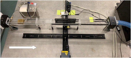
Figure 3 shows the experimental set-up used in this research. The experiments were conducted in a single-channel wind tunnel which is made of Perspex and has a length of 1.75 m, an internal width of 70 mm, and an internal height of 50 mm. A planar PIV system was used to measure the streamwise and vertical velocity components. The flow measurements were conducted at the centre of the channel as indicated by the coordinate system in Figure 2, this means at the centreline of a honeycomb cell.

Figure 3. Experimental set-up of the single-channel wind tunnel used in this research. The white arrow indicates the flow direction of the air. The seeding particles flow through a mixer before entering the 3D printed honeycomb. At the top centre the sCMOS camera is shown with on the other side the double pulsed Nd:YAG laser.

Liquid di-ethyl-hexyl-sebacate (DEHS) droplets generated by a Palas AGF 2.0 aerosol generator were used to seed the flow. The seeding particles were distributed homogeneously by means of a mixer before entering the 3D printed honeycomb. Downstream of the honeycomb a 1 mm thick light sheet was generated by a double pulsed Nd:YAG laser. This means that the relative laser thickness to the hydraulic diameter of the honeycomb cell is around 1/10. The laser light has a wavelength of 532 nm and can be used with a frequency of 15 Hz, which limits the temporal resolution of the PIV measurements. The laser cavities produce laser pulses of 32 mJ at maximum power. A 5.5-megapixel sCMOS camera from LaVision was used to record the individual PIV images with a minimum interframe time of 120 ns. The sCMOS camera and the optical element were mounted on a rail over which they can be translated in the streamwise direction to measure further downstream of the honeycomb. The LaVision software package DaVis 10.1.0 was used to control the equipment and to analyse the measurements. In each measurement, 400 image pairs were recorded with a mean particle displacement of 6 pixels between two images of the same pair. The measurement uncertainty of the root mean square of the streamwise velocity fluctuations $u_{\mathrm{R}\mathrm{M}\mathrm{S}}^{\prime }$ is calculated using 95% confidence interval and was estimated using the normal distribution assumption according to Benedict and Gould [13]. This results in relative error of 6.9%. For the PIV analysis, a multi-pass cross-correlation PIV processing with an interrogation window of $32\times 32$ pixels and an overlap of 75 % was used. This interrogation was chosen after an optimisation study where the effect of the size on the turbulence intensity results was investigated in detail. The obtained vector fields were processed with MATLAB, where the PivMat 4.0.1 toolbox was used to load the DaVisoutput.

2.3. Numerical approach

The fluid is considered as a continuous phase and is treated in an Eulerian way and assumed to be incompressible. Therefore, the fluid satisfies the continuity equation for incompressible flow, (2) $\mathrm{\nabla }\cdot \mathbf{u}=0,$(2) with $\mathbf{u}$ the velocity of the fluid. The fluid momentum equation is modeled by the incompressible Navier-Stokes equation in rotational form, (3) $\frac{\mathrm{\partial }\mathbf{u}}{\mathrm{\partial }t}+\omega \times \mathbf{u}+\mathrm{\nabla }P=\nu \mathrm{\Delta }\mathbf{u}+\mathbf{F},$(3) with $\omega =\mathrm{\nabla }\times \mathbf{u}$ the vorticity, $P=p/{\rho }_f+\frac{1}{2}{\mathbf{u}}^2$, ν the fluid kinematic viscosity, p is the static pressure, ${\rho }_f$ the fluid mass density, and $\mathbf{F}$ the driving force per unit mass, chosen in such a way to sustain a constant bulk velocity.

The computational domain and the corresponding coordinate system are shown in Figure 4. A rectangular domain with dimensions $L_x\times L_y\times L_z$ was used. The walls of the channel are located at y = −L and y = +L. Periodic boundary conditions are used in the streamwise (x) and spanwise (z) direction. The domain is discretised in a uniform way in the streamwise and spanwise directions and in a non-uniform way in the wall-normal direction. The non-uniform mesh is determined via $y_i=\cos \left(i\pi /N_y\right)$, with $y_i$ the coordinate of the grid point, $N_y$ the total number of points in the y-direction and $i=0,\dots ,N_y$. The equations are discretised in space by using a pseudo-spectral method. For the spatial discretisation, a Fourier-Galerkin method is used in the two periodic directions and the Chebyshev-tau method in the wall-normal direction. For the integration in time, a combination of an explicit three-stage Runge–Kutta method and the implicit Crank–Nicholson method is applied. For details of the numerical approach, the reader is referred to Kuerten et al. [14].

Figure 4. Numerical domain with the corresponding coordinate system. Periodic boundary conditions are used in the streamwise (x) and spanwise (z) direction.

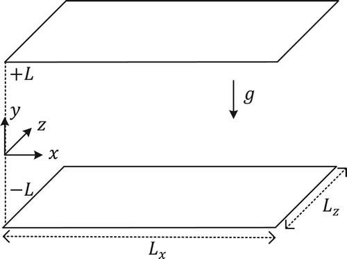
An MDS system usually has moving top and bottom walls to prevent the formation of boundary layers. The governing equations are therefore solved in a frame moving in the streamwise direction with the mean flow velocity $U_{\mathrm{\infty }}$. This is the biggest difference with the experimental set-up, where the walls are stationary.

A consequence of solving the governing equations in a moving frame is that time and streamwise coordinate are swapped in the numerical simulation. This means that time t and streamwise position x can be converted via (4) $t=\frac{x}{U_{\mathrm{\infty }}}.$(4) Similarly, the initial condition of the numerical simulation corresponds to the time-dependent flow quantities at the exit of the honeycomb.

The initial solution depends on whether the flow in a honeycomb cell is laminar or turbulent. For laminar flow in the honeycomb cells, the velocity components are decomposed in a mean $\overline{\mathbf{u}}$ and a fluctuation ${\mathbf{u}}^{\prime }$ via $\mathbf{u}=\overline{\mathbf{u}}+{\mathbf{u}}^{\prime }$, where $\overline{v}$ and $\overline{w}$ are equal to zero due to the fully developed character of the flow. The mean streamwise velocity component $\overline{u}$ is based on an approximation of the analytical expression for laminar flow in a rectangular duct as derived by Shah and London [15] (5) $u(y,z)=U_{cell}\left(\frac{m+1}{m}\right)\left(\frac{n+1}{n}\right)\left[1-{\left(\frac{y}{b}\right)}^n\right]\left[1-{\left(\frac{z}{a}\right)}^n\right],$(5) where m and n are functions of the aspect ratio ${\alpha }^{\ast }$ (6) $\begin{array}{rl}m& =1.8+0.5({\alpha }^{\ast }{)}^{-1.4},\end{array}$(6) (7) $\begin{array}{rl}n& =\left\{\begin{array}{ll}2,& \mathrm{f}\mathrm{o}\mathrm{r}{\alpha }^{\ast }\le 1/3\\ 2+0.3({\alpha }^{\ast }-1/3),& \mathrm{f}\mathrm{o}\mathrm{r}\le 1/3{\alpha }^{\ast }\le \mathrm{0.5.}\end{array}\right.\end{array}$(7) In order to make a realistic comparison with the experiments, the values for $v_0^{\prime }$, $w_0^{\prime }$ and $u_0^{\prime }$ are extracted from the PIV measurements immediately downstream of the honeycomb. The measured velocities are decomposed in different waves with amplitude A and wavenumber k in the vertical direction. Since planar PIV only measures the x- and y- component of the velocity, the fluctuating velocity components are assumed homogeneous and isotropic in the y- and z-direction. It is known that this assumption is not so accurate immediately downstream of the honeycomb. Since the fluctuating velocity field must be divergence free, the third velocity component $w_0^{\prime }$ can be found via $w_0^{\prime }=\int (-\frac{\mathrm{\partial }{u}_0^{\prime }}{\mathrm{\partial }x}-\frac{\mathrm{\partial }{v}_0^{\prime }}{\mathrm{\partial }y})dz$. This results in the following initial conditions (8) $\begin{array}{rl}{u}_0^{\prime }& =+A_{u_1}\sin \frac{2k_{u_1}\pi x}{L_x}\sin \frac{2k_{u_1}\pi y}{H_c}\sin \frac{2k_{u_1}\pi z}{W_c}\\ & -A_{u_2}\sin \frac{2k_{u_2}\pi x}{L_x}\sin \frac{2k_{u_2}\pi y}{H_c}\sin \frac{2k_{u_2}\pi z}{W_c},\\ v_0^{\prime }& =-A_{v_1}\frac{H_c}{W_c}\sin \frac{2k_{v_1}\pi x}{L_x}\sin \frac{2k_{v_1}\pi y}{H_c}\sin \frac{2k_{v_1}\pi z}{W_c}\end{array}$(8) (9) $\begin{array}{rl}& -A_{v_2}\frac{H_c}{W_c}\sin \frac{2k_{v_2}\pi x}{L_x}\sin \frac{2k_{v_2}\pi y}{H_c}\sin \frac{2k_{v_2}\pi z}{W_c},\\ w_0^{\prime }& =+A_{u_1}\frac{W_c}{L_x}\cos \frac{2k_{u_1}\pi x}{L_x}\sin \frac{2k_{u_1}\pi y}{H_c}\cos \frac{2k_{u_1}\pi z}{W_c}\end{array}$(9) (10) $\begin{array}{rl}& -A_{u_2}\frac{W_c}{L_x}\cos \frac{2k_{u_2}\pi x}{L_x}\sin \frac{2k_{u_2}\pi y}{H_c}\cos \frac{2k_{u_2}\pi z}{W_c}\\ & -A_{v_1}\sin \frac{2k_{v_1}\pi x}{L_x}\cos \frac{2k_{v_1}\pi y}{H_c}\cos \frac{2k_{v_1}\pi z}{W_c}\\ & -A_{v_2}\sin \frac{2k_{v_2}\pi x}{L_x}\cos \frac{2k_{v_2}\pi y}{H_c}\cos \frac{2k_{v_2}\pi z}{W_c},\end{array}$(10) with $k_{i_1}$, and $k_{i_2}$ the first two most dominant wavenumbers with amplitude $A_{i_1}$ and $A_{i_2}$. $L_x$, $H_c$ and $W_c$ are, respectively, the length of the computational domain in the x-direction, the cell height and the cell width.

The initial condition for turbulent cases is extracted from a direct numerical simulation (DNS) of fully-developed turbulent duct flow at the same Reynolds number.

For each honeycomb cell, a unique velocity profile is created to break the symmetry. For laminar flow in the honeycomb cells, the amplitudes are randomly varied between $0.1\mathrm{\%}$ and $0.2\mathrm{\%}$ of the measured amplitude. For turbulent flow in the honeycomb cells, the DNS solution is shifted over a random distance in the streamwise direction for every cell.

3. Results and discussions

The wake behind a honeycomb is investigated in three different ways. First, the velocity field and the turbulence intensity fields are shown. Then a more in-depth investigation of production and dissipation of TKE is performed. Finally, a power law for the decay of the turbulence intensity is proposed.

We first show by comparison with experimental results that the numerical simulations provide a faithful representation of reality. From the numerical simulations, the time-series of the streamwise velocity signal will be investigated to show that the flow downstream of the honeycomb is turbulent above a certain value of the Reynolds number, even if the flow in the honeycomb cells is laminar. We subsequently use the numerical results, which are in contrast to the experimental results, not prone to noise, to explore the terms in the turbulence kinetic energy equation.

3.1. Turbulence intensity

An important question is where the turbulence intensity downstream the honeycomb reaches its maximum value and what this maximum value is. The amount of generated turbulence in the wake of the honeycomb is quantified by the turbulence intensity I (11) $I=\frac{\sqrt{\left(u_{RM{S}^2}^{\prime }+v_{RM{S}^2}^{\prime }+w_{RM{S}^2}^{\prime }\right)/3}}{U_{\mathrm{\infty }}},$(11) with $u_{\mathrm{R}\mathrm{M}\mathrm{S}}^{\prime }$ the root mean square of the streamwise velocity fluctuations. The root mean square is determined over N sample measurements of the velocity fluctuations and is defined as (12) $u_{\mathrm{R}\mathrm{M}\mathrm{S}}^{\prime }=\sqrt{\frac{1}{N}\sum _{i=1}^N{u}_{i^2}^{\prime }}.$(12) Since planar PIV can only determine two velocity components, the experimentally measured turbulence intensity will be calculated assuming isotropic behaviour between $v^{\prime }$ and $w^{\prime }$ (13) $I=\frac{\sqrt{\left(u_{RM{S}^2}^{\prime }+2v_{RM{S}^2}^{\prime }\right)/3}}{U_{\mathrm{\infty }}}.$(13) Even though the mean velocity is not isotropic, the fluctuations often are.

3.1.1. Experimental results

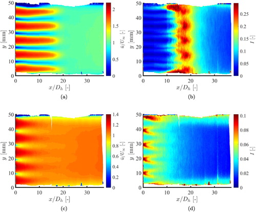
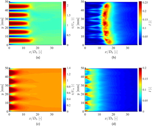
Measurements were performed for 12 different Reynolds numbers ranging from $\mathrm{R}\mathrm{e}=1190$ up to $\mathrm{R}\mathrm{e}=7400$. Figure 5 shows the time-averaged dimensionless velocity field $\overline{u}/U_{\mathrm{\infty }}$ and the turbulence intensity I for a laminar ($\mathrm{R}\mathrm{e}=1890$) and a turbulent ($\mathrm{R}\mathrm{e}=5800$) flow in the honeycomb cells. For the laminar case, it can be seen that the individual channel profiles downstream of the honeycomb gradually develop into one uniform velocity profile. The break-up of the individual channel profiles corresponds with an increase in the turbulence intensity. The turbulence intensity reaches its maximum at a certain dimensionless distance $x/D_h$ and then starts to decay. For the turbulent case, the highest intensity occurs directly behind the walls and deflects further downstream. This behaviour can be explained by the vortex street in the wake of the cell walls.

Figure 5. Experimentally obtained velocity and turbulence intensity field downstream of the honeycomb. (a) and (b) are, respectively, the dimensionless velocity and turbulence intensity field for $\mathrm{R}\mathrm{e}=1890$. (c) and (d) are, respectively, the velocity and turbulence intensity field for $\mathrm{R}\mathrm{e}=5800$.

The effect of the Reynolds number on the dimensionless streamwise velocity $\overline{u}/U_{\mathrm{\infty }}$ and the generated turbulence intensity I is shown in Figure 6, where the data is extracted at the centre of the channel. Since the velocity is measured at the centre of the honeycomb, the velocity immediately downstream of the honeycomb should correspond to the maximum velocity ${\overline{u}}_{max}$ in the honeycomb cell. For a low Reynolds number this dimensionless velocity, after correcting for the solidity, is close to ${\overline{u}}_{max}/U_{cell}=2.096$, which is in agreement with Shah and London [15]. For increasing Reynolds number, $\overline{u}/U_{\mathrm{\infty }}$ decreases until the flow in the cells become turbulent and $\overline{u}/U_{\mathrm{\infty }}$ equals 1.4. The decreasing value of $\overline{u}/U_{\mathrm{\infty }}$ of the laminar flows in the honeycomb cells indicate that the flow is not yet fully developed when exiting the honeycomb. From this data it can be concluded that flow inside the honeycomb cell is turbulent when $\mathrm{R}\mathrm{e}\ge 4500$.

Figure 6. Experimental results for the dimensionless streamwise velocity (a) and turbulence intensity (b) as a function of $x/D_h$ for 12 different Reynolds numbers at the centre of the channel. Due to the flanges between the wind tunnel sections, data is missing between $38<x/D_h<42$ for $\mathrm{R}\mathrm{e}=1190$.

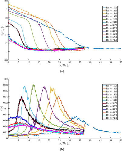
It is clear that the transition towards a uniform velocity profile is associated with an increase in turbulence intensity. For increasing Reynolds number, the position of the turbulence intensity peak moves closer towards the honeycomb, which is in agreement with [9], until the flow in the honeycomb cell is turbulent. If the Reynolds number increases further in the turbulent regime the peak moves away from the honeycomb again. Somewhat similar behaviour can be seen for the maximum intensity. For increasing Reynolds number the maximum grows until the flow in the honeycomb cell reaches the transition region, after which it starts to decrease. For $\mathrm{R}\mathrm{e}\le 2670$ the turbulence intensity immediately downstream of the honeycomb is around I = 0.01. for $\mathrm{R}\mathrm{e}>2670$ the turbulence intensity significantly increases with the Reynolds number. Based on the two observations of $\overline{u}/U_{\mathrm{\infty }}$ and I immediately downstream of the honeycomb, it can be concluded that transition from laminar to turbulent flow in the cells of this honeycomb occurs around $\mathrm{R}\mathrm{e}=3200$.

A low turbulence level in the wake is important for the application of honeycomb laminators to MDS. A maximum turbulence intensity peak position close to the honeycomb is favorable, which can be achieved by using a high Reynolds number. However, the turbulence intensity I is a dimensionless number, which implies that a higher Reynolds number will results in larger velocity fluctuations.

3.1.2. Numerical results

The dimensions of the numerical domain are $L_x=\frac{2}{3}\pi$, $L_y=2$ and $L_z=2.8219$. Nine Reynolds numbers are simulated of which five are in the laminar regime and four in the turbulent regime. As shown in Section 3.1.1, the transition from laminar to turbulent flow in the cells of this honeycomb occurs around $\mathrm{R}\mathrm{e}=3200$. In the numerical approach, a choice has to be made for the state of the initial solution. For $\mathrm{R}\mathrm{e}=3230$ the results will be shown when using both a laminar and a turbulent initial solution. The number of grid points in wall-normal and spanwise directions are 384, and the streamwise direction consists of 128 grid points. In order to enable a direct comparison between experimental and numerical results, the numerical results are made dimensional by using the mass density and viscosity of air at room temperature and the same channel height as in the experiments.

Figure 7 shows the time-averaged dimensionless velocity field $\overline{u}/U_{\mathrm{\infty }}$ and the turbulence intensity I for a laminar ($\mathrm{R}\mathrm{e}=1890$) and a turbulent ($\mathrm{R}\mathrm{e}=5800$) flow. In this figure time and streamwise position are already converted via Equation (4(4) $t=\frac{x}{U_{\mathrm{\infty }}}.$(4) ). The data is extracted at the centreline of the domain in the spanwise direction, which is the same plane as where the experimental data is measured. Since the magnitude of the turbulence intensity of the numerical results is not the same as in the experimental results, the colour scales of Figures 5 and 7 are chosen differently to prevent the loss of visibility of interesting structures. The results show good qualitative agreement with the experimental results shown in Figure 5. Similar features can be observed: for instance, the peak position shifts more towards the left for increasing Reynolds number. Also, the turbulence intensity in the turbulent cases is larger near the honeycomb. Due to the moving top and bottom walls, there is no increasing intensity near the walls, which is in contrast with the experiments.

Figure 7. Numerically obtained dimensionless velocity and turbulence intensity field downstream of the honeycomb. (a) and (b) are, respectively, the velocity and turbulence intensity field for $\mathrm{R}\mathrm{e}=1890$. (c) and (d) are, respectively, the velocity and turbulence intensity field for $\mathrm{R}\mathrm{e}=5800$.

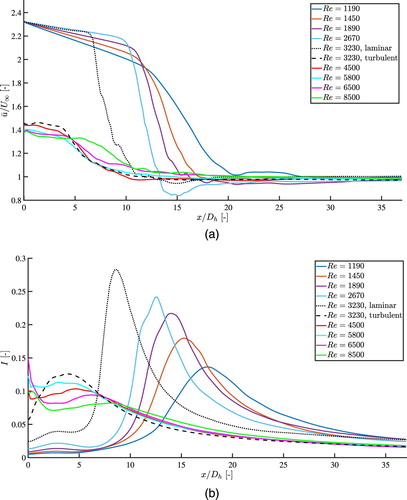
The Reynolds number dependent dimensionless velocity and turbulence intensity are plotted in Figure 8. Since the honeycomb has a symmetric pattern and periodic boundary conditions are used in the z-direction, the results of the turbulence intensity are averaged over the z-direction in order to smoothen the data. This is not done for the dimensionless velocity, otherwise the ratio $\overline{u}/U_{\mathrm{\infty }}$ does not correspond to ${\overline{u}}_{max}/U_{\mathrm{\infty }}$. For the laminar cases $\overline{u}/U_{\mathrm{\infty }}$, after correcting for the solidity, is equal to ${\overline{u}}_{max}/U_{cell}=2.096$. For the turbulent flows ${\overline{u}}_{max}/U_{\mathrm{\infty }}$ equals approximately 1.4. For $\mathrm{R}\mathrm{e}=3230$ the results are dependent on the state of the initial solution. The value of ${\overline{u}}_{max}/U_{cell}$ is close to the characteristic value of the initial flow state, while ${\overline{u}}_{max}/U_{cell}\approx 1.7$ for the experimental results. The turbulence intensity at $x/D_h=0$ for the turbulent initial solution is also found to be higher than in the experiments. A better qualitative agreement with the experimental results is found when using a laminar initial solution for $\mathrm{R}\mathrm{e}=3230$.

Figure 8. Numerical results for the dimensionless streamwise velocity (a) and turbulence intensity (b) as a function of $x/D_h$ for 9 different Reynolds numbers, extracted at the centre of the channel. (b) is averaged over the z-direction to smoothen the data, while (a) is not.

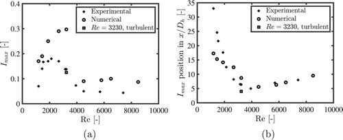
To make a better quantitative comparison between the experimental and numerical result the magnitude and the position of the maximum turbulence intensity at the centre of the channel for the different Reynolds numbers are shown in Figure 9. Similar behaviour for the turbulence intensity peak position and height are noticeable as in the experimental results of Figure 6. Better quantitative agreement cannot be expected, since the break-up of the individual velocity profiles is dependent on details of the flow just behind the honeycomb in the experiments and in the initial condition of the simulations. The magnitude and position of the maximum turbulence intensity at the centre of the channel for $\mathrm{R}\mathrm{e}=3230$ in the case of a turbulent initial solution are indicated by red circles. As can be seen, the results in this transition region depend on the state of the initial solution. The best agreement between experimental and numerical results is obtained if the initial solution of the numerical simulation is turbulent. We conclude that our numerical simulation is a faithful representation of reality and can therefore be used to investigate the complete 3D velocity field.

Figure 9. Experimental and numerical turbulence intensity peak position (a) and peak height (b). For $\mathrm{R}\mathrm{e}=3230$ the circle represents the case with a laminar initial solution, while the  square represents the case with a turbulent initial solution.

3.2. Turbulence kinetic energy budget

Investigating the turbulence kinetic energy budget in the wake of the honeycomb provides insight into the mechanisms for turbulence production and dissipation and increases the physical understanding of this flow. The velocity fluctuations in the honeycomb wake gain and lose energy. Although for low Reynolds numbers the flow is not turbulent everywhere, we will name this energy the turbulence kinetic energy k,defined as (14) $k=\frac{1}{2}\left(\overline{u^{\prime 2}}+\overline{v^{\prime 2}}+\overline{w^{\prime 2}}\right),$(14) which is related to the turbulence intensity by (15) $I=\frac{\sqrt{\frac{2}{3}k}}{U_{\mathrm{\infty }}}.$(15) How the TKE gains and loses its energy is described by the TKE equation given by [16] (16) $\frac{Dk}{Dt}\equiv \frac{\mathrm{\partial }k}{\mathrm{\partial }t}+\overline{u_j}\frac{\mathrm{\partial }k}{\mathrm{\partial }{x}_j}=P_k+T_k+{\mathrm{\Pi }}_k+D_k-ϵ,$(16) with (17) $\begin{array}{rl}& P_k=-\overline{u_i^{\prime }{u}_j^{\prime }}\frac{\mathrm{\partial }\overline{u_i}}{\mathrm{\partial }{x}_j},\end{array}$(17) (18) $\begin{array}{rl}& T_k+{\mathrm{\Pi }}_k+D_k=\frac{\mathrm{\partial }}{\mathrm{\partial }{x}_j}\left(-\overline{u_j^{\prime }{k}^{\prime }}-\frac{1}{{\rho }_0}\overline{p^{\prime }{u}_j^{\prime }}+\nu \frac{\mathrm{\partial }k}{\mathrm{\partial }{x}_j}\right),\end{array}$(18) (19) $\begin{array}{rl}& ϵ=\nu \overline{{\left(\frac{\mathrm{\partial }{u}_i^{\prime }}{\mathrm{\partial }{x}_j}\right)}^2},\end{array}$(19) where i and j are indices for the three directions and summation over repeated indices is assumed. The left-hand side of Equation (16(16) $\frac{Dk}{Dt}\equiv \frac{\mathrm{\partial }k}{\mathrm{\partial }t}+\overline{u_j}\frac{\mathrm{\partial }k}{\mathrm{\partial }{x}_j}=P_k+T_k+{\mathrm{\Pi }}_k+D_k-ϵ,$(16) ) represents the material derivative of the TKE. The terms on the right side are, respectively, the production $P_k$, turbulence diffusion $T_k$, pressure diffusion ${\mathrm{\Pi }}_k$, viscous diffusion $D_k$, and dissipation ϵ.

The advection term ($\overline{u_j}\frac{\mathrm{\partial }k}{\mathrm{\partial }{x}_j}$) represents the convection of the turbulence by the mean flow. The three transport or diffusion terms ($T_k$, ${\mathrm{\Pi }}_k$ and $D_k$) are responsible for the redistribution of the TKE in space due to velocity fluctuations, pressure fluctuations, or viscosity. The production term ($P_k$) acts as a source of TKE. The term represents the interaction of the gradient of the mean flow $\frac{\mathrm{\partial }\overline{u_i}}{\mathrm{\partial }{x}_j}$ and the Reynolds stress $-\overline{u_i^{\prime }{u}_j^{\prime }}$. This gradient of the mean flow can be a shear term (i.e. $\frac{\mathrm{\partial }\overline{u_1}}{\mathrm{\partial }{x}_2}$), or a dilatational term (i.e. $\frac{\mathrm{\partial }\overline{u_1}}{\mathrm{\partial }{x}_1}$). Since shear usually has a higher contribution than dilatation, the production is called shear production. The last term is the dissipation term (ϵ) and acts as a loss term for TKE. TKE is transferred down the energy cascade and is dissipated into heat by the viscous stresses.

The TKE budget terms scales as (20) $\frac{Dk}{Dt}\propto \frac{{\mathcal{L}}^2}{{\mathcal{T}}^3}\propto \frac{{\mathcal{U}}^3}{\mathcal{L}}.$(20) With $\mathcal{T}$ the characteristic time, $\mathcal{L}$ the characteristic length and $\mathcal{U}=\frac{\mathcal{L}}{\mathcal{T}}$ the characteristic velocity. By choosing $\mathcal{U}=U_{\mathrm{\infty }}$ and $\mathcal{L}=D_h$, the terms can be made dimensionless by multiplying them with $D_h/U_{\mathrm{\infty }}^3$.

For the TKE budget we will only investigate the budget of the numerical results. The derivatives of the numerical results are calculated by spectral differences and ensemble averages are taken over the streamwise direction. There are three reasons why we are not able to accurately calculate the individual terms of the TKE from the PIV results. First, we have no information about the pressure which is needed for the pressure transport term ${\mathrm{\Pi }}_k$. Second, filters are needed to prevent the amplification of noise in the TKE budget terms, which will automatically result in reduced accuracy. Third, the dissipation term ϵ needs local velocity derivatives which cannot be accurately determined due to the combination of the PIV resolution and the experimental noise.

The TKE budget as provided by Equation (16(16) $\frac{Dk}{Dt}\equiv \frac{\mathrm{\partial }k}{\mathrm{\partial }t}+\overline{u_j}\frac{\mathrm{\partial }k}{\mathrm{\partial }{x}_j}=P_k+T_k+{\mathrm{\Pi }}_k+D_k-ϵ,$(16) ) is an exact equation that is valid for any flow, irrespective of its state. Identifying ϵ and $P_k$ as the turbulence dissipation and turbulence production is only possible if the flow is turbulent. We investigated the time-series of the streamwise velocity signal from the simulations. The 63 velocity signals are acquired at the centre of 21 channels and at 3 positions close to each other, where the turbulence intensity reaches its maximum. Figure 10 shows the averaged single-sided amplitude spectrum of the time signal for $\mathrm{R}\mathrm{e}=1190$, $\mathrm{R}\mathrm{e}=1890$, $\mathrm{R}\mathrm{e}=3230$ and $\mathrm{R}\mathrm{e}=5800$. For $\mathrm{R}\mathrm{e}=3230$ the results are shown with a laminar initial solution (black lines) and a turbulent initial solution (red lines). We added the $f^{-5/3}$ line to compare the slope of the spectra with that of fully developed turbulence. The slopes of $\mathrm{R}\mathrm{e}=1890$ and the laminar $\mathrm{R}\mathrm{e}=3230$ approach $f^{-5/3}$ while the slopes of the turbulent cases $\mathrm{R}\mathrm{e}=3230$ and $\mathrm{R}\mathrm{e}=5800$ show good agreement with $f^{-5/3}$. For the three higher Reynolds numbers the presence of higher frequencies in the velocity can be observed, which indicates that the flow behaves turbulent. For $\mathrm{R}\mathrm{e}=1190$ the amplitudes are significantly smaller, although the spectrum is also quite broad, and therefore we conclude that the flow is probably not fully turbulent. This means that even though the flow in the honeycomb channels is laminar for $\mathrm{R}\mathrm{e}=1890$, the flow close to the position of maximum turbulence intensity can be treated as turbulent and therefore ϵ and $P_k$ can be identified as the turbulence dissipation and turbulence production.

Figure 10. Single-sided amplitude spectrum of the streamwise velocity time signal for (a) $\mathrm{R}\mathrm{e}=1190$, (b) $\mathrm{R}\mathrm{e}=1890$, (c) $\mathrm{R}\mathrm{e}=3230$ and (d) $\mathrm{R}\mathrm{e}=5800$. In (c) the black lines represent the case with a laminar initial solution, while the dashed line represents the case with a turbulent initial solution. The $f^{-5/3}$ line is added to compare the slope of the spectra with that of fully developed turbulence.

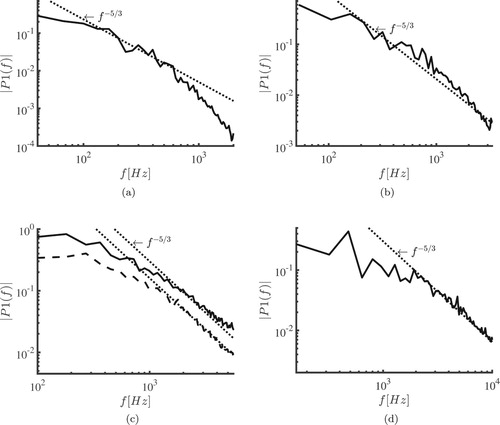
Figure 11 shows the TKE budget for $\mathrm{R}\mathrm{e}=1890$ on the left side and for $\mathrm{R}\mathrm{e}=5800$ on the right side. The data is again averaged over the z-direction. The diffusion terms are disregarded since they only redistribute the TKE and are close to zero when averaged. The terms of the TKE budget show some significant differences between a laminar and a turbulent case. For brevity, only the results of one characteristic laminar case at $\mathrm{R}\mathrm{e}=1890$ and one characteristic turbulent case at $\mathrm{R}\mathrm{e}=5800$ are shown. Other values of the Reynolds number for either laminar or turbulent flow in the honeycomb cells show similar behaviour, but with a different magnitude of the term or a different position where the term has a relevant contribution.

Figure 11. Numerically obtained TKE budget for a laminar and turbulent case of, respectively, $\mathrm{R}\mathrm{e}=1890$ and $\mathrm{R}\mathrm{e}=5800$, (a) Adv term for $\mathrm{R}\mathrm{e}=1890$, (b) Adv term for $\mathrm{R}\mathrm{e}=5800$, (c) $P_k$ for $\mathrm{R}\mathrm{e}=1890$, (d) $P_k$ for $\mathrm{R}\mathrm{e}=5800$, (e) $-ϵ$ for $\mathrm{R}\mathrm{e}=1890$, (f) $-ϵ$ for $\mathrm{R}\mathrm{e}=5800$.

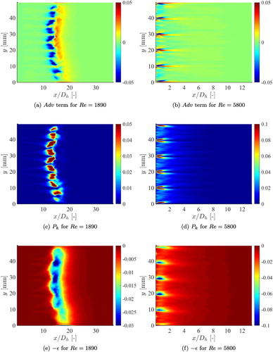
In the laminar case, the production term starts being relevant at the shear layers of the individual channels and develops towards the centre of the channel. The dissipation term shows a more uniform pattern over the total height and is imported further downstream than the production term. The advection term transports the kinetic energy of the honeycomb until it starts to dissipate. This term is proportional to $-\frac{\mathrm{\partial }k}{\mathrm{\partial }{x}_j}$ and is therefore negative when production is dominant and positive when dissipation is dominant.

In the turbulent case, the production terms arise directly behind the walls of the honeycomb cells and deflect further downstream. In contrast to the laminar case, the maximum production is not located in the centre of the cells. This can be explained in the following way. For the turbulent case, there is vortex shedding immediately downstream of the honeycomb walls which results in TKE production. The effect of this is also visible in the turbulent dissipation, which is not uniform over the total height but shows a maximum behind the honeycomb walls. Also, this term deflects until the divergent parts from neighboring walls merge and form one uniform pattern. Since the production and dissipation act in the same region, the advection term does not show a clear pattern as in the laminar case. For the laminar case, vortex shedding either does not take place at all or further downstream.

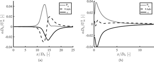
Averaging the production, advection, and dissipation term over the height of one cell results in a TKE budget which is only dependent on the streamwise coordinate. Figure 12 shows these average terms as a function of $x/D_h$. In the laminar case, the production increases as the individual channel profiles slowly start to merge into a uniform flow. At a certain point, the production reaches a maximum and then quickly drops to zero. The advection transports the kinetic energy further downstream until dissipation becomes important. The dissipation slowly decreases towards zero until the flow has become uniform. We verified that the integrals of the production term and the dissipation term are equal. In other words, the energy which is produced is also dissipated. It is interesting to note that the location of the maximum of the production term is slightly upstream of the turbulence intensity peak. In the turbulent case, the flow exiting the honeycomb is already highly turbulent and therefore energy is already dissipated at that position. The production rate is already high at the location of the honeycomb and decreases further downstream. This increase in production does also result in more energy which must be dissipated, which causes the dissipation to increase. The advection term has a different shape than in the laminar case. In the laminar case, the turbulent energy is transported further downstream due to the advection term, which is not so obvious in the turbulent case. This indicates that most of the turbulent energy is dissipated directly after it is produced.

Figure 12. Numerically obtained TKE budget for cell Reynolds number 1890 (a) and 5800 (b). The data is averaged over the z-direction and over the height of one cell. α represents either $P_k$, Adv or $-ϵ$.

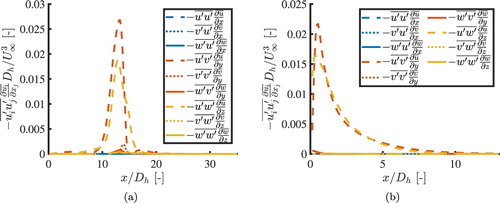
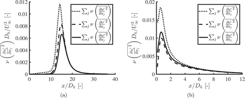
By decomposing the production term in contributions from each velocity gradient, it was investigated how the turbulent energy is produced. Figure 13 shows this decomposition of the production term. In both the laminar and the turbulent case $-\overline{u^{\prime }{v}^{\prime }}\frac{\mathrm{\partial }\overline{u}}{\mathrm{\partial }y}$ and $-\overline{u^{\prime }{w}^{\prime }}\frac{\mathrm{\partial }\overline{u}}{\mathrm{\partial }z}$ have by far the largest contribution. This means that the production of TKE is dominated by the shear layers corresponding to the walls in the y- and z-direction.

Figure 13. Decomposed turbulence production for cell Reynolds numbers 1890 (a) and 5800 (b). The data is averaged over the z-direction and over the height of one cell. In both the laminar and turbulent case the turbulence production is dominated by the shear production terms $-\overline{u^{\prime }{v}^{\prime }}\frac{\mathrm{\partial }\overline{u}}{\mathrm{\partial }y}$ and $-\overline{u^{\prime }{v}^{\prime }}\frac{\mathrm{\partial }\overline{u}}{\mathrm{\partial }z}$.

A similar decomposition can be made for the dissipation terms. In Figure 14 the terms $\nu \left(\overline{{\frac{\mathrm{\partial }{u}^{\prime }}{\mathrm{\partial }{x}_j}}^2}\right)$, $\nu \left(\overline{{\frac{\mathrm{\partial }{v}^{\prime }}{\mathrm{\partial }{x}_j}}^2}\right)$ and $\nu \left(\overline{{\frac{\mathrm{\partial }{w}^{\prime }}{\mathrm{\partial }{x}_j}}^2}\right)$ are shown. Note that the minus sign is ignored. In both the laminar and the turbulent case the biggest contribution to the dissipation term is from the streamwise velocity component. It can also been seen that while the production rate is mostly dominated by one term, $-\overline{u^{\prime }{v}^{\prime }}\frac{\mathrm{\partial }\overline{u}}{\mathrm{\partial }y}$, the dissipation term has significant contributions from all three velocity components. This shows that the fluctuations are more isotropic than the mean flow, but the turbulence of this flow is not homogeneous and isotropic, since the magnitudes of the three dissipation terms are not equal. After around $x/D_h=18$ for the laminar case and $x/D_h=6$ for the turbulent case, the dissipation terms are almost isotropic.

Figure 14. Decomposed turbulence dissipation for cell Reynolds 1890 (a) and 5800 (b). The data is averaged over the z-direction and over the height of one cell.

3.3. Turbulence decay power law

Knowing how the turbulence intensity decays downstream of its maximum value is important for many applications in which a honeycomb is applied to relaminarise a flow. To describe this decay, we follow the methods that are used for the analysis of turbulence generated by grids. However, our goal is not to derive a universally applicable ‘classical’ turbulence decay law, but a decay law that is useful to design a honeycomb that sufficiently reduces the turbulence level downstream and which can be used to predict the turbulence intensity at a specific streamwise position. Our experimental and numerical geometries do not satisfy the requirement for avoiding boundary confinement issues and producing adequate homogeneous isotropic turbulence since it does not have typically 20 or more meshes across the flow [17,18]. This mean that the results are set-up specific and only holds for scaled versions of the same set-up. The width over height ratio of the MDS machine as described in the introduction is in the order of 1000. This means that it has more than 20 meshes in the spanwise direction and is not affected by boundary interference from these walls. Our numerical model has periodic boundary conditions in the spanwise direction and can therefore be used for this application. This does not hold for the experimental set-up which has finite dimensions. The differences between the two set-ups will be discussed.

The power law which applies to the decay of nearly homogeneous and isotropic regions is widely investigated and applied in studies of grid turbulence. An extended form of this decay-law as proposed by Batchelor et al. [19] and Mohamed and LaRue [20] is used (21) $I^2=A{\left(\frac{x-x_0}{D_h}\right)}^p+{\mathcal{N}}^2,$(21) with A the decay coefficient, $x_0$ the virtual origin, p the decay exponent, and $\mathcal{N}$ the noise.

A problem with the decay-law is the wide range of variations of these parameters. Mohamed and LaRue stated that the fit parameters must stay constant while varying the fit range as a function of the downstream position. This procedure is widely used by for example Lavoie et al. [21] and Kurian and Fransson [22]. In addition to this, Mohamed and LaRue also suggested that $x_0/D_h=0$ for square-mesh grids. This value for the virtual origin is often used in grid turbulence by for example Kurian and Fransson [22] and Isaza et al [23]. Lavoie et al. [21] also found values larger than zero for the virtual origin while Djenidi et al. [24] also found negative values.

Isaza et al. [23] performed measurements with a grid and reported two different decay coefficients, one for the near-field decay (p = −1.90) and one for the far-field decay (p = −1.34). Mohamed and LaRue suggested that almost all the data is consistent with p = −1.3. These values are mainly measured in the far-field

Lumley and McMahon [6] and Loehrke [7] investigated the turbulence decay behind a honeycomb, but they did not use the power law as stated in Equation (21(21) $I^2=A{\left(\frac{x-x_0}{D_h}\right)}^p+{\mathcal{N}}^2,$(21) ). However, Lumley and McMahon [6] argued that the decay for a honeycomb is dependent on the drag coefficient $C_D$ of the honeycomb. Incorporating the drag coefficient to scale the turbulence downstream of grids and obstacles is also done by Gomes-Fernandes et al. [25] andSymes [26].

For a honeycomb with laminar flow in the honeycomb cells setting the virtual origin to zero will not work. In grid turbulence the grid acts as a point source for the turbulence, meaning that at this position the production of turbulence is highest. For a honeycomb, the position where the production of TKE is maximum is further away from the honeycomb in case the flow in the honeycomb cells is laminar. The production term averaged over the height of the middle cell is maximum at a position just upstream of the peak in I. This position will be used as the virtual origin and together with a fixed noise, this results in only two unknown parameters, the decay exponent p and the decay coefficient A.

Based on both experimental and numerical results, it will be shown that there is indeed a near- and far-field decay region, but measurements and simulations quite far downstream are required to fully capture the far-field decay. Since measurements in the far-field decay region are not possible for all Reynolds numbers due to the finite size of the wind tunnel, the focus of the analysis will be more on the near-field decay. The two unknown parameters of the decay law will be determined with a least-squares method.

3.3.1. Experimental results

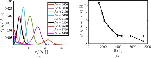
In Section 3.2 it was stated that the TKE budget can not be determined accurately enough from the PIV data. However, this does not hold for the production term. The production term requires the Reynolds stress and the gradient of the mean flow, both terms can be determined accurately without the need for filters. Figure 15 shows the experimental production rates for some of the Reynolds numbers. The positions of the maximum of the production rate are plotted (solid line) as a function of the Reynolds number in Figure 15(a). The virtual origins of the turbulent cases are set to zero since the production rate does not show a clear maximum.

Figure 15. Experimental results: (a) cell averaged production rate as a function of $x/D_h$. The position where the production rate reaches a maximum is used to determine the virtual origin. (b) Virtual origins as a function of the cell Reynolds numbers. The solid line with circular markers correspond to values based on the production rate (Table 2), while the dashed line with triangular markers correspond to values with a fixed decay exponent.

3.3.1.1 Near-field and far-field decay

An experimental investigation of the difference between the near-field and the far-field decay as addressed by Isaza et al. is almost impossible since measurements could only be performed until around $x/D_h=40$ and the noise value has a significant impact on the far-field decay. However, for a cell Reynolds number of 3150, the start of the far-field region is visible. Figure 16 shows the turbulence intensity downstream of the honeycomb for this Reynolds number on a double-logarithmic scale. In Figure 16(b) the square of the turbulence intensity is shown as a function of $(x-x_0)/D_h$ together with fits in the near-field and far-field region. The virtual origin $x_0/D_h$ is based on the maximum production rate and equals 3.67, as will be shown in the next section. As can be seen, due to the lack of data points the far-field is relatively small, and therefore difficult to fit. However, it can still be seen that the near-field decays faster than the far-field. The near-field decays with $p\approx -2.25$ and the far-field with $p\approx -1.16$. Although we apply the power-law to a different situation, our decay exponents are close to the values found by Isaza et al, who reported, respectively, p = −1.9 and p = −1.3 for grid turbulence. All parameters found in the near-field and far-field regions are listed in Table 1.

Figure 16. Downstream evolution of the experimentally obtained turbulence intensity measured at a Reynolds number of 3150. (a) Square of turbulence intensity as a function of $x/D_h$. (b) Square of turbulence intensity (solid line) as a function of $(x-x_0)/D_h$ with the near-field (dash-dotted line) and far-field (dotted line) decay laws found from a power law fit. The virtual origin $x_0/D_h$ is based on the maximum production rate and equals 3.67.

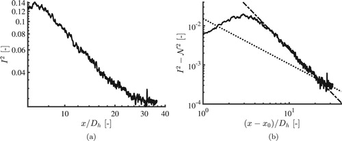
Table 1. Experimentally obtained fit parameters for the near-field and far-field regions for $\mathrm{R}\mathrm{e}\approx 3150$.

Region	p	A	$x_0/D_h$	$\mathcal{N}$
Near-field	−2.25	0.44	3.67	0.016
Far-field	−1.16	0.015	3.67	0.016

Table 2. Experimentally obtained fit parameters with a fixed noise level $\mathcal{N}$ and the virtual origin $x_0/D_h$ based on the position of the maximum production rate.

Re	$\overline{p}$	${\sigma }_p$	$\overline{x_0/D_h}$	$\overline{A}$	${\sigma }_A$	$\overline{\mathcal{N}}$
1450	$-2.12$	0.03	21.51	0.44	0.03	0.008
1890	$-2.00$	0.01	14.98	0.35	0.01	0.009
2130	$-2.04$	0.05	10.35	0.40	0.01	0.011
2670	$-2.20$	0.02	6.27	0.35	0.02	0.015
3150	$-2.29$	0.03	3.67	0.49	0.04	0.016
3230	$-2.10$	0.06	3.67	0.36	0.05	0.016
3930	$-2.18$	0.02	0.00	0.36	0.02	0.011
4500	$-2.13$	0.02	0.00	0.26	0.02	0.007
5700	$-2.12$	0.01	0.00	0.28	0.01	0.006
7400	$-1.74$	0.04	0.00	0.10	0.01	0.011

3.3.1.2 Reynolds-number-dependent near-field fit

For all investigated Reynolds numbers the fitted values of the decay coefficient and decay exponent in the near-field region are presented in Table 2. In all cases the position of the virtual origin is based on the maximum of the production rate and the noise level is determined by performing a measurement far downstream of the honeycomb. While the noise level has a large impact on the determination of the far-field decay, it hardly influences the near-field decay. To make sure that the criterion of Mohamed and LaRue is met, the fit parameters are listed as a mean and standard deviation σ of the fit region. The small standard deviation of the decay coefficient ${\sigma }_p$ shows that the fit meets the criterion of Mohamed and LaRue, that the fit parameters are independent of the fit region. A value of the decay exponent around $-2.1$ is found. The decay exponent for a Reynolds number of 7400 is different from the other ones. This might be caused by the fact that this flow is highly turbulent, so a negative value of the virtual origin is more suitable. The dashed line in Figure 15(b) shows the virtual origin in the case of fixing decay exponent to $-2.1$. The virtual origin for a cell Reynolds number of 7400 becomes negative as expected.

3.3.2. Numerical results

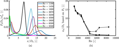
Figure 17 shows the numerically obtained production rates for all the simulated Reynolds numbers. The position of the maximum production rate shows the same behaviour as for the experimental results, but it is not expected that the position will be the same as in the experiments. The numerical simulations do not have noise which is induced by a system and the noise level is therefore set to zero in the procedure to determine the power law.

Figure 17. Numerical results: (a) cell averaged production rate as a function of $x/D_h$. The position where the production rate reaches a maximum is used to fix the virtual origin. (b) Virtual origins as a function of the cell Reynolds numbers. The solid line with circular markers correspond to values based on the production rate (Table 4), while the dashed line with triangular markers correspond to values with a fixed decay exponent.

3.3.2.1 Near-field and far-field decay

For investigating the difference between the near-field and the far-field decay as addressed by Isaza et al., the numerical results with a laminar cell Reynolds number of 3230 will be used. The simulation extends far more downstream than possible in the experiments and there is no noise present. Therefore, the far-field decay can be fitted more accurately. Figure 18 shows the z-averaged turbulence intensity downstream of the honeycomb for this Reynolds number on a double logarithmic scale. At $x/D_h\approx 20$ the decay rate changes from the steeper near-field to the smaller far-field decay. In Figure 16(b) the square of the turbulence intensity is shown as a function of $(x-x_0)/D_h$ together with the near-field and far-field power laws found from the least-squares fit. The virtual origin $x_0/D_h$ was based on the maximum production rate and equals 7.9. The near-field decays with p = −1.89 and the far-field with p = −1.37. Also the numerically found decay exponents are in close agreement with the results of Isaza et al. for grid turbulence [23]. The fit parameters are listed in Table 3.

Figure 18. Downstream evolution of the numerically obtained turbulence intensity measured at $\mathrm{R}\mathrm{e}=3230$ with a laminar initial solution. (a) Square of the turbulence intensity as a function of $x/D_h$. (b) Square of the turbulence intensity squared (solid line) as a function of $(x-x_0)/D_h$ with the near-field (dash-dotted line) and far-field region (dotted line) fitted. The virtual origin $x_0/D_h$ is based on the maximum production rate and equals 7.9.

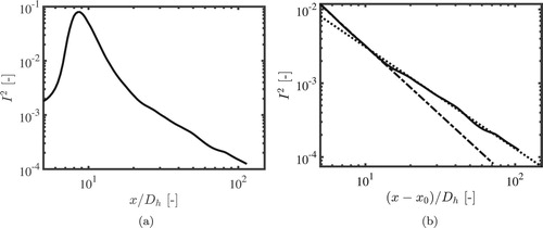
Table 3. Numerically obtained fit parameters for the near-field and far-field regions measured at $\mathrm{R}\mathrm{e}=3230$ with a laminar initial solution.

Region	p	A	$x_0/D_h$	$\mathcal{N}$
Near-field	$-1.89$	0.2487	7.98	0
Far-field	$-1.37$	0.0737	7.98	0

Table 4. Numerically obtained fit parameters, with a fixed virtual origin $x_0/D_h$ based on the maximum production rate.

Re	$\overline{p}$	${\sigma }_p$	$\overline{x_0/D_h}$	$\overline{A}$	${\sigma }_A$
1190	$-1.87$	0.02	17.01	0.21	0.01
1450	$-1.88$	0.03	14.63	0.21	0.01
1890	$-1.82$	0.01	13.14	0.24	0.00
2670	$-1.75$	0.03	11.81	0.18	0.01
3230	$-1.89$	0.02	7.98	0.25	0.01
4500	$-2.00$	0.01	1.03	0.39	0.02
5800	$-2.12$	0.00	0.40	0.60	0.00
6500	$-2.38$	0.00	0.45	1.29	0.01
8500	$-2.36$	0.01	0.29	1.58	0.04

3.3.2.2 Reynolds-number-dependent near-field fit

The fit parameters for the near-field region with the virtual origin set to the position of the maximum production rate are shown in Table 4. For the laminar cases $p\approx -1.9$ is found. For the turbulent cases, the decay exponent is somewhat higher, in contrast to the experimental results.

This means that using the position where the production term of the TKE reaches its maximum as the virtual origin results in a consistent way of describing the decay of the turbulence intensity by a power law. In this way, both the near-field and the far-field decay can be determined for the experimental and numerical results. While the numerical and experiments results are set-up specific, the decay exponents do not differ much from each other. Based on this method it is found that the near-field decays with $p\approx 2$ and the far-field with $p\approx 1.3$. It is also found that for the experimental and numerical results the decay rate is not dependent on the Reynolds number.

4. Conclusions

In this paper, the flow field and turbulence downstream of a honeycomb was investigated experimentally and numerically. For laminar flow inside the honeycomb cells the individual channel profiles downstream of the honeycomb gradually develop into one uniform velocity profile. This development corresponds with an increase in the velocity fluctuations which reaches its maximum and then starts to decay. For turbulent flow inside the honeycomb cells, larger velocity fluctuations occur already directly behind the walls of the honeycomb and the regions of high fluctuations deflect further downstream. The position and magnitude of the turbulence intensity peak depend on the Reynolds number. For increasing Reynolds number, the position of the turbulence intensity peak moves closer towards the honeycomb, until the flow in the honeycomb cells is turbulent. If the Reynolds number increases further in the turbulent regime the peak starts to move away from the honeycomb again. A somewhat similar behaviour can be seen for the maximum intensity. For increasing Reynolds number the maximum turbulence intensity grows until the flow in the honeycomb cells reaches the transition region, and then starts to decrease. The numerical model is a faithful representation of reality and can therefore be used to reproduce the 3D velocity field downstream of a honeycomb.

The generated turbulence intensity downstream of the honeycomb was investigated in more detail through the TKE budget. In the case of a laminar flow in the honeycomb cells, the production term starts to increase as the individual channel profiles slowly start to merge into a uniform flow. At a certain point, the production reaches a maximum and then quickly drops to zero. The advection term in the TKE equation transports the TKE further downstream until it starts to dissipate. In the case of a turbulent cell flow, the behaviour is different. The flow exiting the honeycomb is already turbulent and therefore energy is already dissipated at that position. It was shown that the production of TKE is dominated by the shear layers corresponding to the honeycomb walls. The maximum location of the production term is slightly upstream of the turbulence intensity peak. At the peak location the flow is not homogeneous and isotropic, but it shows this homogeneous and isotropic behaviour slightly downstream of the turbulence intensity peak.

To describe the decay of the turbulence intensity downstream of the honeycomb by a power law, we used the position where the production term of the TKE reaches its maximum as the virtual origin. In this way both the near-field and the far-field decay can be determined for the experimental and numerical results. While the numerical and experiments results are set-up specific, the decay exponents do not differ much from each other. The near-field decay rate is not dependent on the Reynolds number.

A possible topic for future research is a study of the dependence of the results on the dimensions of the honeycomb cell. In this way it is possible to investigate whether $x/D_h$ is the correct non-dimensional parameter and how the results depend on the thickness of the honeycomb walls.

Acknowledgments

We would like to thank technicians G. W. J. M. Oerlemans and J. M. van der Veen and student P. Simons for their work.

Disclosure statement

No potential conflict of interest was reported by the author(s).

Additional information

Funding

This work is part of the research program ‘Innovative Magnetic Density Separation for the optimal use of resources and energy’ with project number 14915, which is partly financed by the Netherlands Organization for Scientific Research (NWO).

Notes

Note: The virtual origin $x_0/D_h$ is based on the maximum production rate position.

Note: The virtual origin $x_0/D_h$ is based on the maximum production rate.

Note: For $\mathrm{R}\mathrm{e}=3230$ a laminar initial solution is used.

References

- Tajfirooz S, Meijer J, Dellaert R et al.. Direct numerical simulation of magneto-Archimedes separation of plastic particles. J. Fluid Mech. 2021;910:A52.
- Umincorp [Internet]. Rotterdam: 2020 [cited 2020 Nov 1]. Available from: http://www.umincorp.com/
- Hu B. Magnetic density separation of polyolefin wastes [dissertation]. Delft: Delft University of Technology; 2014
- Bakker EJ, Rem PC, Fraunholcz N. Upgrading mixed polyolen waste with magnetic density separation. Waste Manag. 2009;29:1712–1717.
- Lumley JL. Passage of a turbulent stream through honeycomb of large length-to-diameter ratio. J Basic Eng. 1964;86:218–220.
- Lumley JL, McMahon JF. Reducing water tunnel turbulence by means of a honeycomb. J Basic Eng. 1967;89:764–770.
- Loehrke RI, Nagib HM. Control of free-Stream turbulence by means of honeycombs: a balance between suppression and generation. J Fluids Eng. 1976;98:342–351.
- Farell C, Youssef S. Experiments on turbulence management using screens and honeycombs. J Fluids Eng. 1996;118:26–32.
- Mikhailova EU, Repik NP, Sosedko YP. Optimal control of free-stream turbulence intensity by means of honeycombs. Fluid Dyn. 1994;29:429–437.
- Xiong W, Kalkühler K, Merzkirch W. Velocity and turbulence measurements downstream of flow conditioners. Flow Meas Instrum. 2003;14:249–260.
- Kühnen J, Scarselli D, Hof B. Relaminarization of pipe flow by means of 3d-printed shaped honeycombs. J Fluids Eng. 2019;141:1–7.
- Kulkarni V, Sahoo N, Chavan SD. Simulation of honeycomb–screen combinations for turbulence management in a subsonic wind tunnel. J Wind Eng Ind Aerodyn. 2011;99:37–45.
- Benedict LH, Gould RD. Towards better uncertainty estimates for turbulence statistics. Exp Fluids. 1996;22:129–136.
- Kuerten JGM, Van der Geld CWM, Geurts BJ. Turbulence modification and heat transfer enhancement by inertial particles in turbulent channel flow. Phys Fluids. 2011;23:123301–1/8.
- Shah RK, London AL. Laminar flow forced convection in ducts. New York (NY): Academic Press; 1978.
- Nieuwstadt FTM, Boersma BJ, Westerweel J. Turbulence: introduction to theory and applications of turbulent flows. Cham (Switzerland): Springer; 2016.
- Corrsin S. Turbulence: experimental methods. Handbuch der Physik. Berlin, Heidelberg:Springer; 1963.
- George WK, Wang H, Wollbald C, et al., Homogeneous turbulence and its relation and its relation to realizable flows. Proceedings 14th Australasian Fluid Mechanics Conference; 2001; Adelaide, Australia
- Batchelor GK, Townsend AA, Taylor GJ. Decay of isotropic turbulence in the initial period. Proc Math Phys Eng Sci. 1948;193:539–558.
- Mohamed MS, LaRue JC. The decay power law in grid-generated turbulence. J Fluid Mech. 1990;219:195–214.
- Lavoie P, Djenidi L, Antonia RA. Effects of initial conditions in decaying turbulence generated by passive grids. J Fluid Mech. 2007;585:395–420.
- Kurian T, Fransson JHM. Grid-generated turbulence revisited. Fluid Dyn Res. 2009;41:021403.
- Isaza JC, Salazar R, Warhaft Z. On grid-generated turbulence in the near- and far field regions. J Fluid Mech. 2014;753:402–426.
- Djenidi L, Kamruzzaman MD, Antonioa RA. Power-law exponent in the transition period of decay in grid turbulence. J Fluid Mech. 2015;779:544–555.
- Gomes-Fernandes R, Ganapathisubramani B, Vassilicos JC. Particle image velocimetry study of fractal-generated turbulence. J Fluid Mech. 2012;711:306–336.
- Symes C, Fink LE. Effects of external turbulence upon the flow past cylinders. In: Fiedler H, editor. Structure and mechanisms of turbulence I. Berlin, Heidelberg: Springer; 1978. p. 86–102.