Effect of high skewness and kurtosis on turbulent channel flow over irregular rough walls

Abstract

The skewness of the roughness height distribution is one of the key topographical parameters that govern roughness effects on wall-bounded turbulence. In this paper mathematical bounds for realisable values of skewness and kurtosis are discussed in the context of irregular multi-scale rough surfaces, which are representative of typical forms of engineering roughness. The properties of a set of irregular rough surfaces fully covered by roughness features with very high positive and negative skewness and high kurtosis are investigated using direct numerical simulations of turbulent channel flow at ${\text{Re}}_{\tau }=395$. While an increase of the roughness function is observed at moderate skewness values in line with empirical predictions and previous results for moderately skewed surfaces, the roughness function saturates at extreme values of skewness. Overall, the roughness effect is found to be more sensitive to skewness over the negative skewness range compared to the positive skewness range. Surface pressure statistics show that for surfaces with extreme skewness fully covered by roughness features extreme pits or peaks do not dominate the roughness effect and that surrounding roughness features (‘background’ roughness) retain a significant influence. This is because, while extreme roughness features emerge as skewness approaches high positive or negative values, they tend to be sparse decreasing their overall impact on the wall-bounded flow.

Keywords:

• Turbulence
• roughness

1. Introduction

While the default assumption in fluid dynamics is that wall-boundaries are smooth, in reality, most surfaces encountered in engineering and geophysical applications exhibit at least some degree of roughness. This is because even for surfaces with an initially high degree of surface finish, the inevitable processes of decay, such erosion or fouling, will result in the formation of roughness on a surface.

Based on early works by Nikuradse [1], Schlichting [2], Colebrook [3], and others, surface roughness significantly affects wall-bounded turbulence provided the roughness features are sufficiently high to interact with the buffer and the log-layer of the flow, i.e. $k_s$, the ‘equivalent sand-grain roughness’ of the surface scaled by the viscous length scale of the flow, falls into the transitionally rough ($5⪅k_s^{+}⪅70$) or fully rough regime ($k_s^{+}⪆70$) [4]. Numerous experimental and numerical studies have shown that not only the height of the roughness features but also their topography influence how strongly a wall-bounded flow is affected by the presence of roughness (see, e.g. recent reviews by Chung et al. [5] and Kadivar et al. [6]).

Many topographical surface parameters have been identified that influence the response of wall-bounded turbulence to roughness. The most dominant parameter is the height of the roughness features, although ‘roughness height’ is a deceptively simple parameter, since the definition of ‘roughness height’ is not straightforward in the context of irregular rough surfaces where multiple roughness height parameters such as the mean roughness height (Sa), rms roughness height (Sq), mean peak-to-valley height ($S{z}_{5\times 5}$), and maximum peak to valley height (Sz) are in use [5–8].

Beyond this primary roughness parameter, further topographical parameters are required to capture secondary topographical aspects that can influence the flow, such as the shape of the height distribution [9–12], the spatial arrangement of roughness features (anisotropy, clustering, regularity vs irregularity, etc.) [11, 13, 14] and the orientation of a rough surface with respect to the dominant flow direction [15].

Two secondary topographical parameters that are known to have a strong influence on the fluid dynamic roughness effect [5] are the skewness of the roughness height distribution Ssk [9, 12, 16] and the frontal solidity ${\lambda }_f$ [2, 17], which is identical – except for a factor of 1/2 – to the (streamwise) effective slope ES [10, 18–20]. The present study investigates the effect of extreme skewness Ssk and the influence of frontal solidity / effective slope will be controlled by keeping this parameter to an approximately constant value.

Figure 1 shows examples for skewness Ssk and kurtosis Sku reported for engineering rough surfaces in the literature. Also shown is the boundary of Pearson's inequality [21] (1) $Ss{k}^2-Sku+1\le 0$(1) which constrains the possible combinations of skewness Ssk and kurtosis Sku. Many surfaces display moderate values of skewness and kurtosis falling into the approximate range of $Ssk\in [-1,+1]$ and $Sku\in [2,5]$. This range of skewness / kurtosis values has been the focus of most previous studies on the topography-dependence of flow over irregular rough surfaces. However, there are also a substantial number of cases where considerably higher skewness and kurtosis values have been reported. Extreme skewness and kurtosis values are typical of the initial stages of surface roughness formation. For example, in the case of fouling processes the sparse deposition of contaminants will result in high kurtosis and high positive skewness values (see, e.g. biofouling by tube worms [22]). This is because in the early stages, most of the surface is still smooth or displays considerably lower levels of roughness, which may have been left behind by other processes such as surface machining and finishing. Contamination-induced deviations from the smooth-wall (or low background-roughness) plane will appear extreme and strongly influence the shape of the height distribution. With increasing contamination, deviations from the smooth-wall / low background-roughness plane become more common and as a result, skewness and kurtosis decrease (see, e.g. barnacle biofouling with increasing coverage [23]). Similarly, in the case of roughness generation processes where material is removed, e.g. due to impact of objects on the surface, the initial pits will appear extreme compared to the rest of the surface resulting in high kurtosis and high negative skewness of the roughness height distribution. As the surface acquires more blemishes over time, kurtosis and skewness will revert to more moderate values.

Considering the data shown in Figure 1 two regions with high kurtosis values can be identified – cases with high kurtosis and high positive skewness and cases with high kurtosis and high negative skewness. The combination of high kurtosis and nearly zero skewness is less prevalent; this is because the processes described above that lead to roughness with high kurtosis tend to result in either high positive skewness (‘additive’ roughness generation) or high negative skewness (‘subtractive’ roughness generation) in their initial stages.

Figure 1. Map of skewness-kurtosis combinations reported for irregular engineering rough surfaces (black circles) adapted from Jelly & Busse [8]. The black line shows the boundary of Pearson's inequality (1(1) $Ss{k}^2-Sku+1\le 0$(1) ). The red squares show the skewness-kurtosis combinations investigated in the current study. The blue dotted line gives the boundary of possible skewness-kurtosis combinations for unimodal distributions (3(3) $Ss{k}^2-Sku+\frac{189}{125}\le 0.$(3) ).

Another observation that can be made from Figure 1 is that, while extreme skewness values do occur for irregular roughness, the limits of Pearson's inequality are not attained, i.e. the skewness values fall significantly below the maximum bound allowed by Pearson's inequality for a given value of kurtosis. This is because for attaining the boundary of Pearson's inequality the height distribution of a surface must be a Bernoulli distribution [24], i.e. a probability distribution where only two possible values can be realised. In the context of a rough surface this can be described as (2) $p(x_3,{\lambda }_p)=\{\begin{array}{ll}1-{\lambda }_p& \mathrm{f}\mathrm{o}\mathrm{r}{x}_3=0\\ {\lambda }_p& \mathrm{f}\mathrm{o}\mathrm{r}{x}_3=k\\ 0& \mathrm{o}\mathrm{t}\mathrm{h}\mathrm{e}\mathrm{r}\mathrm{w}\mathrm{i}\mathrm{s}\mathrm{e}\end{array}$(2) where ${\lambda }_p$ is the fraction of the surface covered by roughness features of uniform height k and $x_3$ is the wall-normal coordinate. While rough surfaces with height distributions that correspond to a Bernoulli distribution do exist, for example, surfaces partially covered by cubes or square bars of uniform height (see, e.g. [25–30]), such surfaces are created by deliberate human design and are not the result of typical surface roughness generation processes encountered in an engineering or geophysical context, such as corrosion, fouling, machining, or erosion. Klaassen, Mokveld & van Es [24] showed that for unimodal distributions, i.e. distributions with one clear peak, as are typically found for irregular rough surfaces, a stricter bound for skewness and kurtosis can be derived resulting in a modified version of Pearson's inequality. (3) $Ss{k}^2-Sku+\frac{189}{125}\le 0.$(3) Therefore, cube and bar roughness of uniform height, which are popular forms of roughness employed in fundamental studies of flow over rough surfaces, are, based on their skewness / kurtosis properties, mathematically in some respects distinct from typical forms of roughness found in engineering and geophysical applications.

While systematic variations of very high skewness and kurtosis values have been previously realised in the context of surfaces generated using roughness elements in the limit of low planform solidities ${\lambda }_p\to 0$ (see, e.g. [2, 23, 31]), these studies typically do not control for the influence of effective slope, since – as the number of roughness elements on a surface is changed - both skewness and effective slope will change simultaneously. The aim of the current study is to systematically investigate the fluid dynamic properties of irregular rough surfaces from moderate to extreme skewness and kurtosis values in the case of homogeneous irregular roughness of approximately constant effective slope. The surfaces considered are rough all over, i.e. extreme peaks (or pits) are surrounded by smaller-scale roughness features.

This paper is structured as follows: In Section 2 details of the surface generation process and the direct numerical simulation approach for obtaining the surfaces' fluid dynamic properties are given. The resulting mean flow and turbulence statistics are presented in Section 3 and discussed in the context of the empirical relationship by Flack & Schultz [9, 16]. Section 4 gives a summary and conclusions.

2. Methodology

In this section, the methodology for the artificial generation of irregular rough surfaces with high skewness and kurtosis is described and the influence of the surface autocorrelation on skewness-kurtosis bounds is discussed. The generated irregular rough surfaces are then characterised using standard surface topographical parameters. This is followed by a discussion of the numerical approach employed in the direct numerical simulations.

2.1. Surface generation

Irregular rough surfaces with increasing positive and negative skewness were generated using the discrete surface generation algorithm of Patir [32] and Bakolas [33] combined with the Fourier-filtering approach by Busse et al. [34]. Together, Patir's and Bakolas' algorithms allow to generate discrete height maps $z_{ij}$ with (nearly) arbitrary skewness and kurtosis and specified discrete 2D surface autocorrelation function (ACF) $R_{pq}$. This is achieved by using a matrix of correlation weights, $c_{kl}$, to generate an $N\times M$ array of correlated random numbers, $z_{ij}$, by applying a $n\times m$ weighted moving average to an $N\times M$ array of uncorrelated random numbers, ${\eta }_{ij}$. In discrete form, this can be expressed as (4) $\begin{array}{r}{z}_{ij}=\sum _{k=1}^n\sum _{l=1}^m{c}_{kl}{\eta }_{rs}\begin{array}{l}i=1,2,\dots ,N\\ j=1,2,\dots ,M\\ r=[(i+k-1)modN]+1\\ s=[(j+l-1)modM]+1\end{array}\end{array}$(4) where mod   denotes the modulo operation. Note that since periodic boundary conditions will be employed in the direct numerical simulations of turbulent channel flow, the surface algorithm by Patir [32] and Bakolas [33] was adapted to generate discrete periodic height maps.

The matrix of coefficients, $c_{kl}$, and the discrete ACF, $R_{pq}$, (both arrays of size $n\times m$) are related through a system of non-linear equations (5) $\begin{array}{r}{R}_{pq}=\sum _{k=1}^{n-p}\sum _{l=1}^{m-q}{c}_{kl}{c}_{k+p,l+q}\begin{array}{l}p=0,1,\dots ,n-1\\ q=0,1,\dots ,m-1\end{array}\end{array}$(5) which is solved numerically using an iterative solver [35].

Arbitrary autocorrelation functions can be employed; in the present study a simple exponentially decaying function was used [32] (6) $R_{pq}=\{\begin{array}{ll}\exp (-2.3\sqrt{{\left({\displaystyle \frac{p}{n-1}}\right)}^2+{\left({\displaystyle \frac{q}{m-1}}\right)}^2})& \mathrm{i}\mathrm{f}p<f_x\left(n\right)\mathrm{a}\mathrm{n}\mathrm{d}q<f_y\left(m\right)\\ 0& \mathrm{o}\mathrm{t}\mathrm{h}\mathrm{e}\mathrm{r}\mathrm{w}\mathrm{i}\mathrm{s}\mathrm{e}\end{array}$(6) where the floor functions (7) $f_x\left(n\right)=\lfloor -\left(\frac{n-1}{2.3}\right)\ln \left(R_{\mathrm{\infty }}\right)\rfloor ,f_y\left(m\right)=\lfloor -\left(\frac{m-1}{2.3}\right)\ln \left(R_{\mathrm{\infty }}\right)\rfloor$(7) return the number of points in the streamwise (n) and spanwise (m) direction in order to achieve a user-specified threshold, $R_{\mathrm{\infty }}$. Throughout this work, a cutoff of $R_{\mathrm{\infty }}=0.001$ was prescribed.

After the coefficients have been determined, an uncorrelated random number matrix, ${\eta }_{ij}$, has to be generated with a specified statistical distribution. If a Gaussian heightmap is desired, then ${\eta }_{ij}$ is generated with a Gaussian distribution $(Ss{k}_{\eta },Sk{u}_{\eta })=(0,3)$. On the other hand, if a non-Gaussian heightmap is desired then ${\eta }_{ij}$ is generated with a non-Gaussian distribution with a specified combination of $Ss{k}_{\eta }$ and $Sk{u}_{\eta }$. Following the recommendations of Bakolas [33] non-Gaussian random number sequences are generated using Johnson's Translator System (JTS) [36]. Given a Gaussian random number input sequence, ζ, JTS returns an output sequence, η, employing three main types of translator curves: (8) $\begin{array}{rl}& S_U:\zeta =\gamma +\delta {\sinh }^{-1}\left(\frac{\eta -\xi }{\lambda }\right)\end{array}$(8) (9) $\begin{array}{rl}& S_L:\zeta =\gamma +\delta \ln \left(\frac{\eta -\xi }{\lambda }\right)(\eta >\xi )\end{array}$(9) (10) $\begin{array}{rl}& S_B:\zeta =\gamma +\delta \ln \left(\frac{\eta -\xi }{\xi +\lambda -\eta }\right)(\xi <\eta <\xi +\lambda )\end{array}$(10) where the parameter set $\{\theta ,\delta ,\xi ,\lambda \}$ is determined via Hill's algorithm [37] in order to select the unbounded $\left(S_U\right)$, log-normal $\left(S_L\right)$, or bounded $\left(S_B\right)$ curve.

Since the heightmap Equation (4(4) $\begin{array}{r}{z}_{ij}=\sum _{k=1}^n\sum _{l=1}^m{c}_{kl}{\eta }_{rs}\begin{array}{l}i=1,2,\dots ,N\\ j=1,2,\dots ,M\\ r=[(i+k-1)modN]+1\\ s=[(j+l-1)modM]+1\end{array}\end{array}$(4) ) is essentially a weighted moving average (MA) process, the relationship between the moments of an input $\left(\eta \right)$ and output (z) random number sequence can be derived explicitly. Following approach by Bakolas [33], the present 2D MA process described by Equation (4(4) $\begin{array}{r}{z}_{ij}=\sum _{k=1}^n\sum _{l=1}^m{c}_{kl}{\eta }_{rs}\begin{array}{l}i=1,2,\dots ,N\\ j=1,2,\dots ,M\\ r=[(i+k-1)modN]+1\\ s=[(j+l-1)modM]+1\end{array}\end{array}$(4) ) can be rewritten as a 1D moving average process (11) $z_I=\sum _{K=0}^{nm-1}{\theta }_K{\eta }_R$(11) by applying a suitable index transform (12) $\left\{\begin{array}{lrl}{z}_I=z_{ij}& \mathrm{w}\mathrm{h}\mathrm{e}\mathrm{r}\mathrm{e}& i=1,\dots ,N;j=1,\dots ,M;I=(i-1)M+(j-1)\\ {\theta }_K=c_{kl}& \mathrm{w}\mathrm{h}\mathrm{e}\mathrm{r}\mathrm{e}& k=1,\dots ,n;l=1,\dots ,m;K=(k-1)m+(l-1)\\ {\eta }_R={\eta }_{rs}& \mathrm{w}\mathrm{h}\mathrm{e}\mathrm{r}\mathrm{e}& r=[(i+k-1)modN]+1;\\ & \mathrm{a}\mathrm{n}\mathrm{d}& s=[(j+l-1)modM]+1;R=(r-1)M+(s-1)\end{array}\right\}$(12) For a 1D moving average process the input and output skewness and kurtosis are related by factors ${\text{β}}_1$ and ${\text{β}}_2$ which are defined as [33, 38] (13) $Ss{k}_z=\underset{{\text{β}}_1}{\underbrace{\left[\frac{\sum _{K=0}^{nm-1}{\theta }_K^3}{{\left(\sum _{K=0}^{nm-1}{\theta }_K^2\right)}^{3/2}}\right]}}Ss{k}_{\eta },Sk{u}_z=\underset{{\text{β}}_2}{\underbrace{\left[\frac{\sum _{K=0}^{nm-1}{\theta }_K^4}{{\left(\sum _{K=0}^{nm-1}{\theta }_K^2\right)}^2}\right]}}(Sk{u}_{\eta }-3)+3.$(13) In Equation  (13(13) $Ss{k}_z=\underset{{\text{β}}_1}{\underbrace{\left[\frac{\sum _{K=0}^{nm-1}{\theta }_K^3}{{\left(\sum _{K=0}^{nm-1}{\theta }_K^2\right)}^{3/2}}\right]}}Ss{k}_{\eta },Sk{u}_z=\underset{{\text{β}}_2}{\underbrace{\left[\frac{\sum _{K=0}^{nm-1}{\theta }_K^4}{{\left(\sum _{K=0}^{nm-1}{\theta }_K^2\right)}^2}\right]}}(Sk{u}_{\eta }-3)+3.$(13) ), $(Ss{k}_{\eta },Sk{u}_{\eta })$ are the skewness and kurtosis of the uncorrelated random number matrix ${\eta }_{ij}$ (Equation  (4(4) $\begin{array}{r}{z}_{ij}=\sum _{k=1}^n\sum _{l=1}^m{c}_{kl}{\eta }_{rs}\begin{array}{l}i=1,2,\dots ,N\\ j=1,2,\dots ,M\\ r=[(i+k-1)modN]+1\\ s=[(j+l-1)modM]+1\end{array}\end{array}$(4) )) required to achieve the desired combination of $Ss{k}_z$ and $Sk{u}_z$ of the correlated discrete heightmap $z_{ij}$. Since $|{\theta }_K|\le 1$, the rescaling factors $({\text{β}}_1,{\text{β}}_2)\le 1$ and hence $(⏐Ss{k}_{\eta }⏐,⏐Sk{u}_{\eta }-3⏐)\ge (⏐Ss{k}_z⏐,⏐Sk{u}_z-3⏐)$, i.e. the output skewness and kurtosis will revert to less extreme values (closer to a normal distribution) compared to the input skewness and kurtosis.

Since the magnitude of the rescaling factors $({\text{β}}_1,{\text{β}}_2)$ in Equation (13(13) $Ss{k}_z=\underset{{\text{β}}_1}{\underbrace{\left[\frac{\sum _{K=0}^{nm-1}{\theta }_K^3}{{\left(\sum _{K=0}^{nm-1}{\theta }_K^2\right)}^{3/2}}\right]}}Ss{k}_{\eta },Sk{u}_z=\underset{{\text{β}}_2}{\underbrace{\left[\frac{\sum _{K=0}^{nm-1}{\theta }_K^4}{{\left(\sum _{K=0}^{nm-1}{\theta }_K^2\right)}^2}\right]}}(Sk{u}_{\eta }-3)+3.$(13) ) is determined by the coefficients ${\alpha }_{kl}$, realisable combinations of $(Ss{k}_z,Sk{u}_z)$ depend on the specified ACF. This can be seen by recasting Pearson's inequality (1(1) $Ss{k}^2-Sku+1\le 0$(1) ) in terms of $Ss{k}_z={\text{β}}_{1}Ss{k}_{\eta }$ and $Sk{u}_z={\text{β}}_2(Sk{u}_{\eta }-3)+3$ to obtain (14) $(Ss{k}_z{)}^2\le {\text{β}}_1^2[\frac{1}{{\text{β}}_2}(Sk{u}_z-3)+2]$(14) where the lower bound on $Sk{u}_z$ is (15) $min\left(Sk{u}_z\right)=3-2{\text{β}}_2$(15) The bounds on $(Ss{k}_z,Sk{u}_z)$ for a general ACF are determined by inequality (14(14) $(Ss{k}_z{)}^2\le {\text{β}}_1^2[\frac{1}{{\text{β}}_2}(Sk{u}_z-3)+2]$(14) ) and Equation (15(15) $min\left(Sk{u}_z\right)=3-2{\text{β}}_2$(15) ) – provided the coefficients ${\alpha }_{kl}$ and rescaling factors ${\text{β}}_1$ and ${\text{β}}_2$ are known.

In the simple case of a linear autocorrelation matrix [32] (16) $R_{pq}=\{\begin{array}{ll}(1-{\displaystyle \frac{p}{n}})(1-{\displaystyle \frac{q}{m}})& \mathrm{f}\mathrm{o}\mathrm{r}p<n\mathrm{a}\mathrm{n}\mathrm{d}q<m\\ 0& \mathrm{o}\mathrm{t}\mathrm{h}\mathrm{e}\mathrm{r}\mathrm{w}\mathrm{i}\mathrm{s}\mathrm{e}\end{array}$(16) the correlation weights are constant and the coefficient matrix can be expressed as (17) $c_{kl}=\frac{1}{\sqrt{nm}}$(17) After substituting (17(17) $c_{kl}=\frac{1}{\sqrt{nm}}$(17) ) into Equation (13(13) $Ss{k}_z=\underset{{\text{β}}_1}{\underbrace{\left[\frac{\sum _{K=0}^{nm-1}{\theta }_K^3}{{\left(\sum _{K=0}^{nm-1}{\theta }_K^2\right)}^{3/2}}\right]}}Ss{k}_{\eta },Sk{u}_z=\underset{{\text{β}}_2}{\underbrace{\left[\frac{\sum _{K=0}^{nm-1}{\theta }_K^4}{{\left(\sum _{K=0}^{nm-1}{\theta }_K^2\right)}^2}\right]}}(Sk{u}_{\eta }-3)+3.$(13) ), the inequality (14(14) $(Ss{k}_z{)}^2\le {\text{β}}_1^2[\frac{1}{{\text{β}}_2}(Sk{u}_z-3)+2]$(14) ) simplifies to (18) $(Ss{k}_{z,\mathrm{l}\mathrm{i}\mathrm{n}}{)}^2\le (Sk{u}_{z,\mathrm{l}\mathrm{i}\mathrm{n}}-3)+\frac{2}{nm}$(18) where the lower bound on $Sk{u}_z$ is (19) $min\left(Sk{u}_{z,\mathrm{l}\mathrm{i}\mathrm{n}}\right)=3-\frac{2}{nm}$(19) In the limit of a perfectly decorrelated surface ($nm\to 1$), inequality (18(18) $(Ss{k}_{z,\mathrm{l}\mathrm{i}\mathrm{n}}{)}^2\le (Sk{u}_{z,\mathrm{l}\mathrm{i}\mathrm{n}}-3)+\frac{2}{nm}$(18) ) reduces to Pearson's inequality (1(1) $Ss{k}^2-Sku+1\le 0$(1) ) and sets the theoretical boundary for uncorrelated random variables which is attained in the limit of binary white noise. However, since the majority of naturally existing roughness has finite correlation length $(1<nm<\mathrm{\infty })$, the skewness-kurtosis combinations of physical roughness specimens cannot land close to Pearson's theoretical limit (1(1) $Ss{k}^2-Sku+1\le 0$(1) ) both because their height distributions are not Bernoulli distributions as discussed above and the fact that they have finite autocorrelation.

In summary, the moving averaging process will decrease the absolute excess kurtosis and the absolute value of the skewness. This needs to be taken into account when specifying input skewness $Ss{k}_{\eta }$ and kurtosis $Sk{u}_{\eta }$ using the JTS. The degree of change between input and output skewness and kurtosis is influenced by the chosen form of autocorrelation function and correlation lengths. Furthermore, the susceptibility of skewness and kurtosis to finite size sampling effects needs to be considered [39], i.e. the ideal theoretical relationship between input and output skewness and kurtosis is reliably attained only in the case of infinitely large random number arrays.

In a final step, which does not form part of Patir's and Bakolas' algorithm, the discrete surfaces, $z_{ij}$, are filtered using a circular low-pass Fourier filter with a cut-off wave number of $k_c=40$ to create continuous and differentiable heightmaps, $h(x_1,x_2)$, similar to the low-pass filtering approach previously applied to surface scans [34]. It should be noted that this step results in a further reduction of absolute skewness and kurtosis since extreme surface features are reduced by low-pass filtering.

2.2. Topographies of the generated surfaces

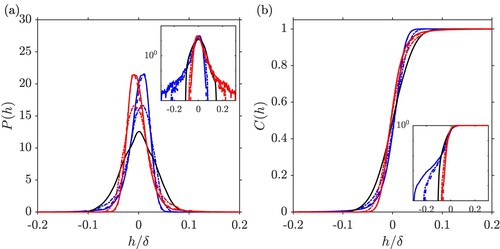
In the present study, four different surfaces were generated using the methodology described in the previous section. This includes a surface with an approximately Gaussian height distribution which will be used as a reference case (see Figure 2(a)) and three surfaces with increasing kurtosis and increasing negative skewness (see Figure 2(b–d)). Based on these three negatively skewed surfaces three positively skewed counter-parts were generated by mirroring them with respect to the horizontal $(x_1-x_2-)$ plane (see Figure 2(e–g)). The corresponding probability density and cumulative distribution functions are shown in Figure 3.

Key topographical parameters of all surfaces are given in Table 1. All surfaces have been scaled to the same mean peak to valley height $S{z}_{5\times 5}/\delta =1/6$ and a surface size of $8\delta \times 4\delta$, where δ is the mean channel half-height, was used in all cases. Corresponding surface heights and sizes were successfully used in previous DNS studies on irregular anisotropic roughness [13] and Reynolds number-dependency of irregular roughness [8] for neutrally skewed surfaces generated using the same methodology. The mean-peak-to-valley height was chosen as characteristic length scale in line with previous results, which showed that this length scale tends to be for isotropic irregular roughness much closer in magnitude to the equivalent sand-grain roughness of a surface than height measures such as the mean roughness height Sa or rms roughness height Sq [40, 41]. Since the mean-peak-to valley height is the fixed height scale, other height scales such as the rms roughness height Sq decrease as the absolute skewness and kurtosis is increased. Furthermore, the streamwise effective slope of all surfaces was limited to approximately $0.2\pm 0.01$ to minimise the influence of this parameter. The spanwise effective slope was also kept close to 0.2, meaning that all surfaces are statistically isotropic which allows to exclude the effects of anisotropy in the present study. The only parameters in which the surfaces vary significantly between each other are the higher moments of the height distribution, i.e. skewness and kurtosis. The skewness and kurtosis combinations investigated in the current study have been included in the map shown in Figure 1 and are representative of surfaces with very high positive or negative skewness and high kurtosis reported in the literature.

Figure 2. Visualisations of the generated irregular rough surfaces. First row: Gaussian reference surface; second row: negatively skewed surfaces from left to right in order of increasing $⏐Ssk⏐$; third row: positively skewed surfaces from left to right in order of increasing Ssk.

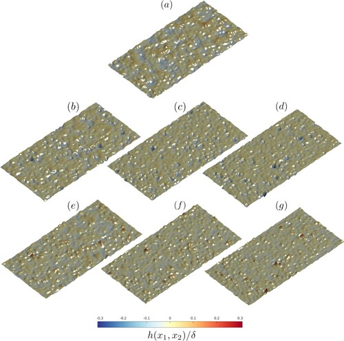
Figure 3. (a) Probability density functions and (b) cumulative distribution functions of $h(x,y)$ of the surfaces shown in Figure 2. Line styles are given in Table 2. The inset plots show the same data with a logarithmic y-axis.

2.3. Direct numerical simulations

Direct numerical simulations (DNS) of incompressible turbulent channel flow were used to investigate the fluid dynamic properties of the generate rough surfaces. All simulations were conducted at ${\text{Re}}_{\tau }=\delta u_{\tau }/\nu =395$ where δ is the mean channel half-height, $u_{\tau }$ the friction velocity based on the constant mean streamwise pressure gradient driving the flow, and ν the kinematic viscosity. The rough surfaces were applied to both sides of the~channel to ensure statistical symmetry with respect to the channel centre plane. The upper rough surface corresponds to a shifted mirror image of the lower surface. The applied shift corresponds to half of the domain size in the streamwise and spanwise direction to minimise local blockage effects. Periodic boundary conditions are applied in the streamwise and spanwise direction. The inherently periodic surface generation process ensures that there are no steps or other artefacts in the surfaces at the periodic boundaries. To resolve the flow past the irregular rough surfaces an iterative version of the embedded boundary method of Yang & Balaras [42] was employed on a structured grid; second order centred differences are used for the spatial discretisation and the second order Adams-Bashforth method for the time-advancement. Details of the computational approach applied can be found in reference [34].

Table 1. Key topographical parameters of the surfaces investigated in the current DNS.

Name	$Sa/\delta$	$Sq/\delta$	$S{z}_{5\times 5}/\delta$	Ssk	Sku	$E{S}_x$	$E{S}_y$	$S_{max}/\delta$	$S_{min}/\delta$
Gaussian	0.0263	0.0330	0.167	0.0	3.0	0.209	0.220	$+0.1429$	$-0.0996$
skew_p1p0	0.0205	0.0269	0.167	$+1.0$	5.8	0.204	0.207	$+0.2239$	$-0.0735$
skew_m1p0	0.0205	0.0269	0.167	$-1.0$	5.8	0.204	0.207	$+0.0735$	$-0.2239$
skew_p1p5	0.0173	0.0234	0.167	$+1.5$	8.0	0.204	0.203	$+0.2126$	$-0.0605$
skew_m1p5	0.0173	0.0234	0.167	$-1.5$	8.0	0.204	0.204	$+0.0605$	$-0.2126$
skew_p2p3	0.0168	0.0237	0.167	$+2.3$	17.0	0.198	0.195	$+0.3044$	$-0.0749$
skew_m2p3	0.0168	0.0237	0.167	$-2.3$	17.0	0.198	0.195	$+0.0749$	$-0.3044$

Notes: Sa – mean roughness height; Sq – rms roughness height; $S{z}_{5\times 5}$ mean peak-to-valley height; Ssk – surface skewness; Sku – surface kurtosis; $E{S}_x$ – streamwise effective slope; $E{S}_y$ – spanwise effective slope; $S_{max}$ - maximum height; $S_{min}$ – minimum height.

Table 2. Simulation parameters for the current rough-wall channel flow DNS.

case	$L_1$	$L_2$	$L_3$	$n_1\times n_2\times n_3$	$\mathrm{\Delta }{x}_1^{+}$	$\mathrm{\Delta }{x}_2^{+}$	$\mathrm{\Delta }{x}_{3,min}^{+}$	$\mathrm{\Delta }{x}_{3,max}^{+}$	line style
Gaussian	8	4	2	$640\times 320\times 576$	4.94	4.94	0.667	4.04	$\text{-}$
skew_p1p0	8	4	2	$640\times 320\times 576$	4.94	4.94	0.667	4.92	$red\text{–}$
skew_m1p0	8	4	2	$640\times 320\times 624$	4.94	4.94	0.667	4.80	$blue\text{‐}$
skew_p1p5	8	4	2	$640\times 320\times 576$	4.94	4.94	0.667	4.66	$red\text{‐}$
skew_m1p5	8	4	2	$640\times 320\times 624$	4.94	4.94	0.667	4.59	$blue\text{‐}$
skew_p2p3	8	4	2	$640\times 320\times 672$	4.94	4.94	0.667	4.40	$red\text{-}$
skew_m2p3	8	4	2	$640\times 320\times 720$	4.94	4.94	0.667	4.96	$blue\text{-}$
smooth	8	4	2	$640\times 320\times 360$	4.94	4.94	0.50	3.98	$\circ \circ \circ \circ$

Notes: $L_1$: streamwise domain size; $L_2$: spanwise domain size; $L_3$: mean channel height; $n_1\times n_2\times n_3$: number of grid points; $\mathrm{\Delta }{x}_1^{+}$: grid-spacing in streamwise direction; $\mathrm{\Delta }{x}_2^{+}$ grid-spacing in spanwise direction; $\mathrm{\Delta }{x}_{3,min}^{+}$: minimum wall-normal grid-spacing; $\mathrm{\Delta }{x}_{3,max}^{+}$: maximum wall-normal grid-spacing.

Key simulation parameters are summarised in Table 2. Uniform grid spacing was set in the streamwise and spanwise direction at $\mathrm{\Delta }{x}_1^{+}=\mathrm{\Delta }{x}_2^{+}\le 5$ meeting standard resolution criteria for rough-wall flows. This resolution also ensures that the shortest wavelengths remaining in the surface after the low-pass filtering are resolved by 16 grid points following a criterion developed in the context of simulation of flow over filtered surface scans [43]. In the wall-normal direction, uniform grid spacing at $\mathrm{\Delta }{x}_{3,min}^{+}=0.667$ was used across the height of the roughness. Above, the wall-normal grid spacing was gradually increased reaching its maximum $\mathrm{\Delta }{x}_{3,max}^{+}$ at the channel centre; the maximum wall-normal grid-spacing was kept below $\mathrm{\Delta }{x}_{3,max}^{+}<5$ in all cases. Also included in Table 2 are the corresponding parameters from a previous smooth-wall simulation at ${\text{Re}}_{\tau }=395$ for a matching domain size [13].

In the following, $\overline{\cdot }$ is used to indicate the time average. Mean flow and turbulence statistics were time-averaged in excess of 62 flow through times $L_1/\overline{U}$ (where $\overline{U}$ is the bulk flow velocity) or 44 large-eddy time scales $\delta /u_{\tau }$. Triangular brackets $〈\cdot 〉$ are used to indicate the spatial average over wall-parallel ($x_1$-$x_2$) planes. For the spatial average the intrinsic average was used which is defined for an arbitrary scalar variable $\varphi (x_1,x_2,x_3,t)$ as (20) $〈\overline{\varphi }〉\left(x_3\right)=\frac{{\int }_0^{L_1}{\int }_0^{L_2}c(x_1,x_2,x_3)\overline{\varphi (x_1,x_2,x_3)}\mathrm{d}{x}_2\mathrm{d}{x}_1}{{\int }_0^{L_1}{\int }_0^{L_2}c(x_1,x_2,x_3)\mathrm{d}{x}_2\mathrm{d}{x}_1}$(20) where $c(x_1,x_2,x_3)$ is set to 1 in fluid occupied areas and to 0 in the solid areas.

3. Results and discussion

In this section, mean flow and turbulence statistics obtained from the direct numerical simulations are discussed. In Section 3.1 the mean velocity profiles are presented. The dependency of roughness function and estimated equivalent sand-grain roughness on the surface skewness are evaluated in Section 3.2 and compared to predictions by an empirical relationship. Reynolds stress and dispersive stress statistics are shown in Section 3.3. In Section 3.4 insight into the reasons for the observed saturation of the roughness function at extreme skewness is obtained by considering surface pressure statistics.

3.1. Mean velocity profile

The mean streamwise velocity profile is shown Figure 4(a). As nominal wall reference location ($x_3=0$) for the rough-wall cases the roughness mean plane $〈h(x_1,x_2)〉$, i.e. a geometry based condition, was used [44]. This wall reference location yields an excellent collapse of the outer-layer of the velocity defect and Reynolds stress profiles on the smooth-wall reference case (see below). In all rough cases, the slope in the logarithmic region is similar to the smooth-wall reference case and therefore no zero-plane displacement was applied to the velocity profiles. The difference between the smooth wall and the rough wall profiles (shown in the inset in Figure 4(a)) is approximately constant above the highest roughness crest.

As expected, all surfaces induce a clear roughness effect as is evident from the downwards shift in the mean streamwise velocity profiles compared to the smooth-wall profile. The roughness effect is higher for the positively skewed surfaces than for the negatively skewed surfaces which is in line with previous results on skewness-dependency of rough-wall flows [9, 11, 12, 45]. In all cases, the velocity profile in defect form (see Figure 4(b)) shows a very good collapse on the smooth wall case, indicating that outer-layer similarity of the velocity profile is recovered.

Figure 4. (a) Mean streamwise velocity profile; the inset shows the local downwards shift, i.e. the difference between the smooth-wall and the rough-wall velocity profile vs the wall-normal coordinate; (b) Velocity defect profile; the inset shows the difference between the smooth-wall and rough-wall velocity defect profile. Line styles are given in Table 2.

The recovery of outer-layer similarity is further supported by considering the difference between the smooth-wall and the rough-wall defect profiles (shown in the inset in Figure 4(b)), which is close to zero above the highest roughness crest. This shows that the high peaks for the positively skewed surfaces only affect the flow locally but do not change the global behaviour of the velocity defect profile. This can be explained by considering that while surfaces with high skewness tend to exhibit high peaks, these high peaks occur rarely, i.e. are sparse. While a high peak will alter the local flow behaviour significantly by inducing a velocity defect in its wake, due to sparseness of high peaks, their effect is not substantial enough to distort the shape of the averaged velocity profile.

3.2. Roughness function

The roughness function $\mathrm{\Delta }{U}^{+}$, shown in Figure 5(a) was measured based on the average difference between the mean streamwise velocities between the smooth and the rough wall case for $x_3/\delta >0.5$ (see Table 3). In all cases, a significant roughness effect is observed, and the measured values fall into the mid to upper transitionally rough regime. For moderate skewness, i.e. in the range $-1.5\le Ssk\le 1$ an increase in the roughness function with skewness can be observed. However, surprisingly, with further increase in the absolute skewness value, the roughness function starts to saturate. The present data approximately follows the shape of a hyperbolic tangent function (shown as the dashed line in Figure 5(a)). (21) $\mathrm{\Delta }{U}^{+}=a\mathrm{t}\mathrm{a}\mathrm{n}\mathrm{h}(Ssk+b)+c$(21) with the fitting constants a = 1.39, b = 0.67 and c = 5.11. The shift b>0 indicates that for the present set of surfaces $\mathrm{\Delta }{U}^{+}$ is more sensitive to negative than to positive skewness values. The above fit is not intended as an empirical relationship for the prediction roughness effects since it does not capture the dependency on other relevant topographical parameters such as the roughness height.

An important empirical relationship for the skewness dependence was developed by Flack & Schultz [9] and later refined based on additional experimental data [16]. This relationship relates the equivalent sand-grain roughness to the rms roughness height Sq and the surface skewness Ssk: (22) $k_s=\alpha Sq(\gamma +Ssk{)}^{\text{β}},\mathrm{w}\mathrm{h}\mathrm{e}\mathrm{r}\mathrm{e}\{\begin{array}{lr}\alpha =2.48,\text{β}=2.24,\gamma =1& \mathrm{f}\mathrm{o}\mathrm{r}Ssk>0,\\ \alpha =2.11,\text{β}=0,\gamma =1& \mathrm{f}\mathrm{o}\mathrm{r}Ssk=0,\\ \alpha =2.73,\text{β}=-0.45,\gamma =2& \mathrm{f}\mathrm{o}\mathrm{r}Ssk<0.\end{array}$(22) α, β, and γ are empirical constants that depend on whether a surface is positively, negatively, or neutrally skewed. To be able to compare the present data to this relationship we estimate the equivalent sand-grain roughness based on the roughness function based on the expected behaviour in the fully rough limit [5] (23) $\frac{k_s}{k}=\frac{\exp \left(\kappa (\mathrm{\Delta }{U}^{+}-A+B_s(\mathrm{\infty }\left)\right)\right)}{k^{+}}$(23) where $\kappa \approx 0.4$ and $A-B_s\left(\mathrm{\infty }\right)\approx -3.5$. Since the present cases are not all in the fully rough limit, the above relationship provides merely an estimate, but the resulting values should give a reasonable indication of the expected trends of $k_s$ with extreme skewness.

Figure 5. (a) Roughness function vs surface skewness. The black dashed line shows the fit given in Equation (21(21) $\mathrm{\Delta }{U}^{+}=a\mathrm{t}\mathrm{a}\mathrm{n}\mathrm{h}(Ssk+b)+c$(21) ). (b) Estimated equivalent sand-grain roughness normalised by rms roughness height vs skewness. The corresponding behaviour predicted by the empirical relationship (22(22) $k_s=\alpha Sq(\gamma +Ssk{)}^{\text{β}},\mathrm{w}\mathrm{h}\mathrm{e}\mathrm{r}\mathrm{e}\{\begin{array}{lr}\alpha =2.48,\text{β}=2.24,\gamma =1& \mathrm{f}\mathrm{o}\mathrm{r}Ssk>0,\\ \alpha =2.11,\text{β}=0,\gamma =1& \mathrm{f}\mathrm{o}\mathrm{r}Ssk=0,\\ \alpha =2.73,\text{β}=-0.45,\gamma =2& \mathrm{f}\mathrm{o}\mathrm{r}Ssk<0.\end{array}$(22) ) is also shown - blue line: negative skewness branch; red line: positive skewness branch; black cross: neutral skewness condition.

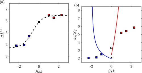
Table 3. Mean flow quantities measured for the present surfaces.

case	$U_c$	$\overline{U}$	${\text{Re}}_c$	$\text{Re}$	$\mathrm{\Delta }{U}^{+}$	$F_p/F_{tot}$
Gaussian	14.30	11.73	5,647	9,267	5.93	0.53
skew_p1p0	13.72	11.51	5,421	8,810	6.54	0.53
skew_m1p0	15.55	12.86	6,144	10,160	4.73	0.47
skew_p1p5	14.01	11.34	5,534	8,972	6.29	0.51
skew_m1p5	16.32	13.60	6,445	10,744	3.97	0.44
skew_p2p3	13.76	11.17	5,436	8,824	6.52	0.54
skew_m2p3	16.37	13.63	6,465	10,773	3.93	0.43
smooth	20.92	17.57	8,015	13,882	–	0.0

Notes: $U_c$: centreline velocity; $\overline{U}$: bulk flow velocity; ${\text{Re}}_c=\delta U_c/\nu$: Reynolds number based on centreline velocity; $\text{Re}=2\delta \overline{U}/\nu$: Reynolds number based on bulk flow velocity; $\mathrm{\Delta }{U}^{+}$: roughness function; $F_p/F_{tot}$ fractional pressure drag contribution.

Results for the estimated equivalent sand-grain roughness normalised by the rms roughness height are shown in Figure 5(b) and compared to the behaviour predicted by the empirical relationship (22(22) $k_s=\alpha Sq(\gamma +Ssk{)}^{\text{β}},\mathrm{w}\mathrm{h}\mathrm{e}\mathrm{r}\mathrm{e}\{\begin{array}{lr}\alpha =2.48,\text{β}=2.24,\gamma =1& \mathrm{f}\mathrm{o}\mathrm{r}Ssk>0,\\ \alpha =2.11,\text{β}=0,\gamma =1& \mathrm{f}\mathrm{o}\mathrm{r}Ssk=0,\\ \alpha =2.73,\text{β}=-0.45,\gamma =2& \mathrm{f}\mathrm{o}\mathrm{r}Ssk<0.\end{array}$(22) ). In the present cases, the positively skewed surfaces show a much more gradual increase of the roughness effect with Ssk than predicted by the empirical correlation. The disagreement in the negatively skewed cases is even stronger. Here the empirical relationship predicts a rapid increase of $k_s$ as skewness approaches $-2$, whereas for the present cases $k_s$ decreases and approaches an approximately constant value.

The empirical relationship (22(22) $k_s=\alpha Sq(\gamma +Ssk{)}^{\text{β}},\mathrm{w}\mathrm{h}\mathrm{e}\mathrm{r}\mathrm{e}\{\begin{array}{lr}\alpha =2.48,\text{β}=2.24,\gamma =1& \mathrm{f}\mathrm{o}\mathrm{r}Ssk>0,\\ \alpha =2.11,\text{β}=0,\gamma =1& \mathrm{f}\mathrm{o}\mathrm{r}Ssk=0,\\ \alpha =2.73,\text{β}=-0.45,\gamma =2& \mathrm{f}\mathrm{o}\mathrm{r}Ssk<0.\end{array}$(22) ) was derived based on data with moderate skewness ($-1⪅Ssk⪅1$) and in its present form it has limitations when applied to cases with more extreme skewness. The most obvious limitation is that it is not defined for surfaces with high negative skewness $Ssk\le -2$; to allow a relationship in the form (22(22) $k_s=\alpha Sq(\gamma +Ssk{)}^{\text{β}},\mathrm{w}\mathrm{h}\mathrm{e}\mathrm{r}\mathrm{e}\{\begin{array}{lr}\alpha =2.48,\text{β}=2.24,\gamma =1& \mathrm{f}\mathrm{o}\mathrm{r}Ssk>0,\\ \alpha =2.11,\text{β}=0,\gamma =1& \mathrm{f}\mathrm{o}\mathrm{r}Ssk=0,\\ \alpha =2.73,\text{β}=-0.45,\gamma =2& \mathrm{f}\mathrm{o}\mathrm{r}Ssk<0.\end{array}$(22) ) to be applied for all negative skewness values, $Ssk=-\mathrm{\infty }\dots 0$, the empirical constant γ must be less than zero. In the positive skewness case, the relationship predicts that the equivalent sand-grain roughness will rapidly approach infinity as Ssk is increased assuming constant Sq. However, this is unlikely to be the correct limiting behaviour. If we for example consider the simple case of rough surfaces constructed by placing cubical roughness elements of uniform height k on a smooth surface (which corresponds to Bernoulli-type roughness height distribution (2(2) $p(x_3,{\lambda }_p)=\{\begin{array}{ll}1-{\lambda }_p& \mathrm{f}\mathrm{o}\mathrm{r}{x}_3=0\\ {\lambda }_p& \mathrm{f}\mathrm{o}\mathrm{r}{x}_3=k\\ 0& \mathrm{o}\mathrm{t}\mathrm{h}\mathrm{e}\mathrm{r}\mathrm{w}\mathrm{i}\mathrm{s}\mathrm{e}\end{array}$(2) )), then the rms roughness height of the surface will vary as (24) $Sq\left({\lambda }_p\right)=k{\lambda }_p^{1/2}{(1-{\lambda }_p)}^{1/2}$(24) with the planform solidity ${\lambda }_p$ (i.e, the percentage of the surface covered by the roughness elements) and the skewness as (25) $Ssk\left({\lambda }_p\right)=\frac{1-2{\lambda }_p}{{\left[{\lambda }_p\right(1-{\lambda }_p\left)\right]}^{1/2}}.$(25) In the extreme limit of very low coverage (${\lambda }_p\to 0$) and extreme skewness ($Ssk\to \mathrm{\infty }$), where the cubes are infinitely spaced apart, we would expect the equivalent sand-grain roughness to approach zero $k_s\to 0$. This implies for any relationship of the form (26) $k_s=\alpha Sq(\gamma +Ssk{)}^{\text{β}}\underset{{\lambda }_p\to 0}{\sim }SqSs{k}^{\text{β}}$(26) that the Ssk term can only be taken to a power less than one ($\text{β}<1$) to allow $k_s$ to approach zero since in the limit ${\lambda }_p\to 0$, rms roughness height and skewness behave asymptotically as $Sq\sim {\lambda }_p^{1/2}$ and $Ssk\sim {\lambda }_p^{-1/2}$. Similarly, if we consider the extreme limit of negative skewness in the case of a rough surface constructed from extremely densely spaced cubes of uniform height we would expect the equivalent sand grain roughness to approach zero as the coverage approaches 100% (${\lambda }_p\to 1$) since in the limit of full coverage the cubes will merge to form a smooth surface. This in turn also places a constraint for the exponent of $\text{β}<1$ since for ${\lambda }_p\to 1$ rms roughness height and skewness behave asymptotically as $Sq\sim (1-{\lambda }_p{)}^{1/2}$ and $Ssk\sim -(1-{\lambda }_p{)}^{-1/2}$.

3.3. Reynolds and dispersive stress statistics

The spatio-temporal variations of the velocity field can be split into the turbulent fluctuations around the local mean value (27) $u_i^{\mathrm{\prime }}(\overrightarrow{x},t)=u_i(\overrightarrow{x},t)-{\overline{u}}_i\left(\overrightarrow{x}\right)$(27) which give rise to the Reynolds stresses $〈u_i^{\mathrm{\prime }}{u}_j^{\mathrm{\prime }}〉$, and the spatial variation of the time-averaged fields (28) ${\tilde{u}}_i\left(\overrightarrow{x}\right)={\overline{u}}_i\left(\overrightarrow{x}\right)-〈{\overline{u}}_i〉\left(x_3\right)$(28) which give rise to the dispersive stresses $〈{\tilde{u}}_i{\tilde{u}}_j〉$ [46]. The streamwise Reynolds stresses (see Figure 6(a)) exhibit a clear reduction in their peak values for all rough cases. Above the highest roughness crest a good collapse on the smooth-wall reference case can be observed. This also applies to all other Reynolds stress components. The peak magnitude, shown in the inset, decreases further the higher the roughness effect of the surface. A decrease in the peak value with increasing skewness was for example also observed by Kuwata & Kawaguchi [45] who covered the skewness range $Ssk\in [-1,+1]$ in their study. However, as for the roughness function, a saturation of the peak value at the extreme end of skewness can be observed – there is little difference in the peak value when comparing the Ssk = −2.3 and Ssk = −1.5 cases, and at the other extreme, the peak value does not decrease much further when skewness is increased above 1.

Figure 6. (a) Streamwise Reynolds stresses; (b) streamwise dispersive stresses; line styles are given in Table 2. The abscissae have been clipped to the range $[-0.2,1.0]$. The inset plots show the maxima as a function of the surface skewness Ssk.

Figure 7. Visualisations of time-averaged streamwise velocity in plane $x_3/\delta =0.05$. First row: Gaussian reference surface; second row: negatively skewed surfaces from left to right in order of increasing $⏐Ssk⏐$; third row: positively skewed surfaces from left to right in order of increasing Ssk.

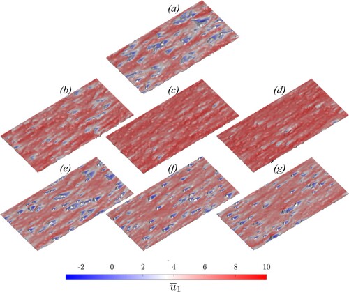
Figure 8. (a) Spanwise Reynolds stresses; (b) spanwise dispersive stresses; line styles are given in Table 2. The abscissae have been clipped to the range $[-0.2,1.0]$. The inset plots show the maxima as a function of the surface skewness Ssk.

Figure 9. (a) Wall-normal Reynolds stresses; (b) wall-normal dispersive stresses; line styles are given in Table 2. The abscissae have been clipped to the range $[-0.2,1.0]$. The inset plots show the maxima as a function of the surface skewness Ssk. For the dispersive stress case, the maximum values are based on the outer maxima ($max(〈{\tilde{u}}_3{\tilde{u}}_3〉(x_3>0\left)\right)$).

Figure 10. (a) Reynolds shear stress; (b) dispersive shear stress; line styles are given in Table 2. The abscissae have been clipped to the range $[-0.2,1.0]$. The inset plots show the maxima as a function of the surface skewness Ssk.

Substantial streamwise dispersive stresses can be observed for all cases (see Figure 6) which arise from the spatial variation in the time-averaged streamwise velocity field (see Figure 7 for illustration). When considering the peak values, the neutrally skewed case gives rise to the highest streamwise dispersive stress values, whereas significantly lower values occur both for high positive and negative skewness. The lower peak values for the negatively skewed surfaces can be explained by that fact that the bulk flow interacts less strongly with the rough surface, since it largely passes by the deep cavities that are occupied by recirculating flows. The lower peak values for the positively skewed cases may be a result of the fact that, while the high peaks of these surfaces do induce substantial dispersive stresses above the roughness mean plane, around the roughness mean plane these surfaces show a larger areas with lower roughness features compared to the Gaussian case.

The profiles of the spanwise Reynolds stresses, shown in Figure 8(a), are in comparison only little changed by the presence of the roughness. There is a very good collapse of all cases on the smooth-wall reference data above the highest roughness peak. The negatively skewed cases show slightly elevated values, but the difference compared to the positively skewed cases is small. More distinct behaviour can be seen in the spanwise dispersive stress profiles presented in Figure 8(b). The peaks for the negatively skewed cases occur below the roughness mean plane and can be associated with the three-dimensional recirculating flow patterns within the pronounced cavities of these surfaces. However, it should be noted that at the low $x_3$ locations where the spanwise dispersive stress peaks for the negatively and neutrally skewed cases are observed, the intrinsic average (20(20) $〈\overline{\varphi }〉\left(x_3\right)=\frac{{\int }_0^{L_1}{\int }_0^{L_2}c(x_1,x_2,x_3)\overline{\varphi (x_1,x_2,x_3)}\mathrm{d}{x}_2\mathrm{d}{x}_1}{{\int }_0^{L_1}{\int }_0^{L_2}c(x_1,x_2,x_3)\mathrm{d}{x}_2\mathrm{d}{x}_1}$(20) ) is computed over small fluid occupied areas (less than $10\mathrm{\%}$ of $L_1\times L_2$, see Figure 3(b)) and thus the dependence of the peak magnitude on skewness is not statistically significant. In contrast, the peaks for the positively skewed cases fall slightly above the roughness mean plane, where averages are taken over larger fluid occupied areas, and can be related to time-averaged flow patterns such as the in-plane circumnavigation of high peaks. As for the streamwise dispersive stresses, a decrease in the peak levels with increasing positive skewness can be observed. The negatively skewed surfaces still contain some obstacles that induce spanwise dispersive stresses as a result of the flow passing them, and the negatively skewed cases therefore still retain significant spanwise dispersive stress levels above the roughness mean plane.

The wall-normal Reynolds stresses (see Figure 9(a)) are – like their spanwise counterpart – little changed by the rough surfaces. Peak levels are slightly elevated for the positively skewed cases – a moderate increase in the peak level can be observed with increasing positive skewness. Finite wall-normal velocity fluctuations can be observed within the deep pits of the negatively skewed surfaces, indicating that the separated flows within the deep pits still retain some unsteadiness. Wall-normal dispersive stress levels, shown in Figure 9(b), are comparatively high for the negatively skewed surfaces indicating the presence of strong recirculating flows within the deep roughness pits. The negatively skewed cases do show a double peak structure in their wall-normal dispersive stress profiles, a second peak can be observed above the roughness mean plane. For the neutrally and positively skewed cases, the peak wall-normal dispersive stress is always located above the roughness mean plane. The peaks above the roughness mean plane can be associated with the up- and downwards motion of the time-averaged flow as it passes over roughness features; this peak is highest for the neutrally skewed case.

For the Reynolds shear stress (see Figure 10) a decreasing trend of the peak level can be observed with increasing skewness. This is consistent with the higher roughness effect of the positively skewed cases. Negative values for the dispersive shear stress $-〈{\tilde{u}}_1{\tilde{u}}_3〉$ occur within the deep cavities of the negatively skewed surfaces which can be associated with the recirculating flow patterns induced in the pits by the bulk flow passing above them. At the roughness mean plane and above, the dispersive shear stress becomes positive. The maximum dispersive shear stress value increases with increasing skewness but appears to saturate at high positive skewness.

3.4. Surface pressure fields

To associate physical mechanisms to changes in the Hama roughness function (Figure 5(a)), the total drag force was partitioned into its pressure and viscous components. After some manipulation, the mean pressure and viscous forces per unit area acting on the surface can be expressed as [47] (29) $\begin{array}{rl}〈F_p〉& ={\iint }_S\left[({\overline{p}}_s-{\overline{p}}_0)\frac{\mathrm{\partial }h}{\mathrm{\partial }{x}_1}\right]\frac{1}{\Vert \mathrm{\nabla }h\Vert }\mathrm{d}S\end{array}$(29) (30) $\begin{array}{rl}〈F_{\nu }〉& ={\iint }_S-\mu (\frac{\mathrm{\partial }{\overline{u}}_1}{\mathrm{\partial }{x}_j}+\frac{\mathrm{\partial }{\overline{u}}_j}{\mathrm{\partial }{x}_1})\frac{\mathrm{\nabla }h}{\Vert \mathrm{\nabla }h\Vert }\mathrm{d}S\end{array}$(30) In Equations (29(29) $\begin{array}{rl}〈F_p〉& ={\iint }_S\left[({\overline{p}}_s-{\overline{p}}_0)\frac{\mathrm{\partial }h}{\mathrm{\partial }{x}_1}\right]\frac{1}{\Vert \mathrm{\nabla }h\Vert }\mathrm{d}S\end{array}$(29) ) and (30(30) $\begin{array}{rl}〈F_{\nu }〉& ={\iint }_S-\mu (\frac{\mathrm{\partial }{\overline{u}}_1}{\mathrm{\partial }{x}_j}+\frac{\mathrm{\partial }{\overline{u}}_j}{\mathrm{\partial }{x}_1})\frac{\mathrm{\nabla }h}{\Vert \mathrm{\nabla }h\Vert }\mathrm{d}S\end{array}$(30) ), ${\overline{p}}_0$ is an arbitrary gauge pressure, taken here as the average surface pressure, i.e. ${\overline{p}}_0\equiv A^{-1}\iint {\overline{p}}_s(x_1,x_2)\mathrm{d}A$, $\mathrm{\nabla }h$ is gradient of the height map, $\Vert \mathrm{\nabla }h\Vert$ is the magnitude of the surface normal vector, and $\mathrm{d}S$ is the incremental surface area. For DNS with constant pressure gradient forcing, the mean hydrodynamic force balance can be expressed as $〈F_p〉+〈F_{\nu }〉=1$ (where $\mathrm{\Pi }=-1$). Hence, the total drag remains fixed, but the fractional contributions of $〈F_p〉$ and $〈F_{\nu }〉$ are free to vary.

Figure 11. Fractional contribution of pressure drag vs (a) surface skewness and (b) Hama roughness function. The grey triangles show data for a pit-peak decomposed surface ($Ssk=\pm 1.62$, $E{S}_x=0.17$) [12] for comparison.

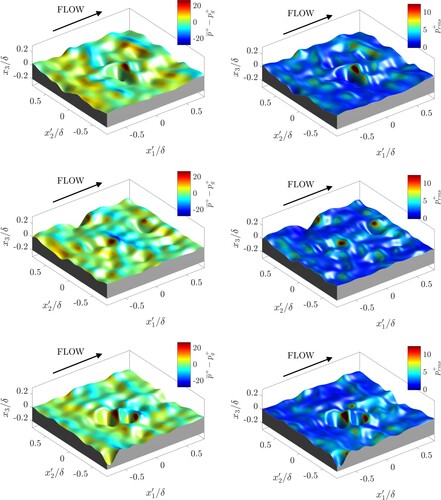
Figure 12. Surface pressure distributions for $Ssk\ge 0$ centred about the highest peak. Left column: time-averaged pressure on surface; right column: time-averaged pressure fluctuations at surface. From top to bottom: Ssk = +2.3, Ssk = +1.5, Ssk = +1.0, and Ssk = 0.0.

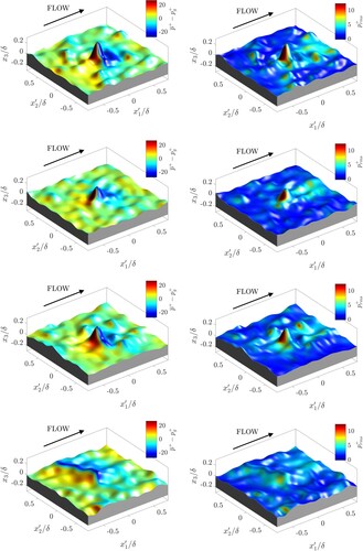
Figure 13. Surface pressure distributions for Ssk<0 centred about the highest peak. Left column: time-averaged pressure on surface; right column: time-averaged pressure fluctuations at surface. From top to bottom: Ssk = −1.0, Ssk = −1.5, and Ssk = −2.3.

The fractional contribution of pressure drag to total drag, $F_p/F_{tot}$, is plotted as a function of surface skewness in Figure 11(a). Pressure drag accounts for approximately $40\mathrm{\%}-55\mathrm{\%}$ of the total drag in all cases. Based on the criterion by Scaggs et al. [48], who defined a 60% pressure drag contribution as the threshold between the transitionally to fully rough regime, the roughness effects of all surfaces in the present study fall into the mid to upper transitionally rough region, but are not quite fully rough at the present Reynolds number. As expected, the pressure drag contribution for the negatively skewed cases is lower than for the positively skewed cases, but it remains appreciable. Overall, the variation of pressure drag data with respect to skewness resembles the Hama roughness function data (Figure 5(a)), in the sense that $F_p$ shows a weakened sensitivity with respect to skewness at the most extreme values of Ssk considered here.

The fractional contribution of pressure drag to total drag, $F_p/F_{tot}$, is plotted versus $\mathrm{\Delta }{U}^{+}$ in Figure 11(b). An approximately linear dependency between $F_p/F_{tot}$ and $\mathrm{\Delta }{U}^{+}$ can be observed for the negatively skewed to neutrally skewed cases. For the positively skewed cases, which result all in approximately in the same value for the roughness function, a higher scatter can be seen in the relationship between $\mathrm{\Delta }{U}^{+}$ and $F_p/F_{tot}$. An approximately linear dependency between the fractional contribution of the pressure drag and the roughness function has previously been observed for irregular rough surfaces with different streamwise and spanwise effective slopes and approximately Gaussian height distributions [47].

The surface pressure distributions (see Figure 12) give insight why the highly positively skewed cases do not exhibit much higher pressure drag contributions than the Gaussian and the negatively skewed cases. While the pronounced peaks of the positively skewed cases will result locally in high pressure differences and high levels of pressure fluctuations on the exposed windward surfaces of the peaks, these peaks are surrounded by relatively low surface undulations which make only weak contributions to the pressure drag. In contrast, the Gaussian surface does not display extreme peaks like the positively skewed cases, however, in compensation, it does exhibit a more ‘rugged terrain’ overall (to keep a comparable effective slope) and since neighbouring peaks tend to have lower differences in height, they can effectively function collectively as transverse ridge-like structures that locally deflect the flow. This results in more moderate pressure drag contributions compared to the extreme peaks of the positive cases which, however, sum up to a substantial pressure drag contribution for the surface overall.

The negatively skewed surfaces also show interesting behaviour in their local surface pressure distributions (see Figure 13). We would expect the bulk flow to have much weaker interaction with these surfaces. However, the outer-flow tends to interact with the lip surrounding a pit, inducing locally higher pressure differences on the surface and high-pressure fluctuations on the windward face of the downstream part of the lip. Transverse-ridge like behaviour of the lower peaks that these surfaces exhibit can also be observed (to a lesser degree than in the Gaussian case), which further contributes to the pressure drag.

The importance of lower roughness features surrounding the pits can be reinforced by considering the pressure drag contribution for a strongly negatively skewed pitted surface where the pits are surrounded by smooth surface sections. To this end, data from an earlier pit-peak decomposition study [12] (which also used DNS of turbulent channel flow at ${\text{Re}}_{\tau }=395$) have been included in Figure 11 for comparison. Since the pitted and the peaked surface from this study had slightly lower effective slope ($Ssk=\pm 1.62$ and $E{S}_x=0.17$) we would expect them to exhibit a slightly lower pressure drag contribution. This is the case for the peaked surface, but the pitted case shows a much lower pressure drag contribution than the present negatively skewed cases. This can be attributed to the fact that the surface parts surrounding the pits in the pitted surface from the decomposition study are smooth whereas in the present cases the pits are surrounded by lower-scale roughness features. This shows that not only the extrema of a rough surface have a strong influence on the roughness effect, but that lower scale roughness features can also have a strong summative effect on the drag, especially in the case of strongly negatively skewed surfaces.

4. Summary and conclusions

Irregular rough surfaces with very high skewness and kurtosis were investigated both by considering theoretical limits on skewness-kurtosis combinations from an analytical viewpoint and by investigating the fluid dynamic behaviour of a set of surfaces with extreme values of skewness $Ssk=-2.3\dots +2.3$ and kurtosis $Sku=3\dots 17$ using direct numerical simulations of turbulent channel flow. A saturation of the roughness effect was observed in the limits of very high positive and very high negative skewness. This saturation is not captured by the widely referenced empirical relationship of Flack & Schultz [9, 16] which was developed in the context of more moderately skewed surfaces $Ssk\approx -1\dots +1$. Limits were derived for the power-law exponent for the skewness in a relationship of the form proposed by Flack & Schultz by considering the extreme case of Bernoulli roughness. Mean flow statistics show that while there are clear effects of the extreme peaks of the positively skewed cases on the local flow field, their impact on the shape of the mean flow velocity profile is not dominant and outer-layer similarity is not impaired. The streamwise Reynolds stresses, which make the largest contribution to the turbulent kinetic energy, saturate both at high positive and high negative skewness values. Most dispersive stress components attain their highest peaks in the Gaussian case and peak values tend to be lower for more highly skewed surfaces. This also shows while surfaces with extreme features will introduce locally very high deviations in the time-averaged fields, these deviations only affect a small part of the flow due to the relative sparseness of extreme features.

Despite the wide range of skewness covered, the pressure drag contributions of all surfaces are of similar magnitude. This is because the drag of a rough surface is not only governed by its extrema but its overall character also needs to be taken into account. While high (positive or negative) skewness and kurtosis is typically caused by extreme features these features tend to be rare since extreme skewness / kurtosis and sparsity tend to go hand in hand. This has the consequence that other parts of the rough surface surface, i.e. the area surrounding the extreme features, can also play an important role in determining the fluid dynamic roughness effect of a rough surface.

In future work, conditional statistics could be employed to investigate the effects of the extreme peaks on the local spatio-temporal structure of the turbulent flow, e.g. to detect vortex-shedding phenomena in the wake of the extreme peaks of highly positively skewed surfaces. Furthermore, it would be of interest to compare the effect of extreme features, i.e. high peaks or deep pits, in different contexts, e.g, peaks (or pits) surrounded by a smooth surface compared to peaks (or pits) surrounded by surfaces with a moderate level of roughness to determine the relative impact of the extreme features and the surrounding background roughness features on the near-wall turbulent structures.

Disclosure statement

No potential conflict of interest was reported by the author(s).

Additional information

Funding

This work used the Cirrus UK National Tier-2 HPC Service at EPCC (https://www.cirrus.ac.uk) funded by the University of Edinburgh and EPSRC [grant number EP/P020267/1]. A. B. gratefully acknowledges support by  a Leverhulme Trust Research Fellowship. Roughness height maps and velocity statistics are available in .csv format at https://doi.org/10.5525/gla.researchdata.1394

References

- Nikuradse J. Strömungsgesetze in Rauhen Rohren. VDI Forschungsheft. 1933;361:1–22.
- Schlichting H. Experimentelle untersuchungen zum rauhigkeitsproblem. Ingenieur-Archiv. 1936;7(1):1–34.
- Colebrook CF, White CM. Experiments with fluid friction in roughened pipes. Proc Roy Soc Lond A. 1937;161(906):367–381.
- Schlichting H, Gersten K. Boundary layer theory. 8th revised and enlarged edition, Berlin Heidelberg: Springer; 2003.
- Chung D, Hutchins N, Schultz MP, et al. Predicting the drag of rough surfaces. Annu Rev Fluid Mech. 2021;53(1):439–471.
- Kadivar M, Tormey D, McGranaghan G. A review on turbulent flow over rough surfaces: fundamentals and theories. Int J Thermofluid. 2021;10:100077.
- Blateyron F. Characterisation of areal surface texture. Springer; 2013. Chapter The Areal Field Parameters; p. 15–43.
- Jelly TO, Busse A. Reynolds number dependence of Reynolds and dispersive stresses in turbulent channel flow past irregular near-Gaussian roughness. Int J Heat Fluid Flow. 2019;80:108485.
- Flack KA, Schultz MP. Roughness effects on wall-bounded turbulent flows. Physics Fluids. 2014;26(10):101305.
- Thakkar M, Busse A, Sandham ND. Surface correlation of hydrodynamic drag for transitionally rough engineering surfaces. J Turbul. 2017;18(2):138–169.
- Forooghi P, Stroh A, Magagnato F, et al. Toward a universal roughness correlation. J Fluids Eng. 2017;139(12):121201.
- Jelly TO, Busse A. Reynolds and dispersive stress contributions above highly skewed roughness. J Fluid Mech. 2018;852:710–724.
- Busse A, Jelly TO. Influence of surface anisotropy on turbulent flow over irregular roughness. Flow Turbul Combust. 2020;104(2–3):331–354.
- Sarakinos S, Busse A. Influence of spatial distribution of roughness elements on turbulent flow past a biofouled surface. In: Proceedings of the 11th International Symposium on Turbulence and Shear Flow Phenomena(TSFP11); 2019.
- Busse A, Zhdanov O. Direct numerical simulations of turbulent channel flow over ratchet roughness. Flow Turbul Combust. 2022;109(4):1195–1213.
- Flack KA, Schultz MP, Barros JM. Skin friction measurements of systematically-varied roughness: probing the role of roughness amplitude and skewness. Flow Turbul Combust. 2019;104(2–3):317–329.
- Jiménez J. Turbulent flow over rough walls. Annu Rev Fluid Mech. 2004;36(1):173–196.
- Napoli E, Armenio V, De Marchis M. The effect of the slope of irregularly distributed roughness elements on turbulent wall-bounded flows. J Fluid Mech. 2008;613:385–394.
- Schultz MP, Flack KA. Turbulent boundary layers on a systematically varied rough wall. Physics Fluids. 2009;21(1):015104.
- Yuan J, Piomelli P. Estimation and prediction of the roughness function on realistic surfaces. J Turbul. 2014;15(6):350–365.
- Pearson K. Mathematical contributions to the theory of evolution. XIX. second supplement to a memoir on skew variation. Philos Trans Royal Soc A. 1916;216:429–457.
- Monty JP, Dogan E, Hanson R, et al. An assessment of the ship drag penalty arising from light calcareous tubeworm fouling. Biofouling. 2016;32(4):451–464.
- Sarakinos S, Busse A. Investigation of rough-wall turbulence over barnacle roughness with increasing solidity using direct numerical simulations. Phys Rev Fluids. 2022;7(6):064602.
- Klaassen CA, Mokveld PJ, van Es B. Squared skewness minus kurtosis bounded by 186/125 for unimodal distributions. Stat Probab Lett. 2000;50(2):131–135.
- Coceal O, Thomas TG, Castro IP, et al. Mean flow and turbulence statistics over groups of urban-like cubical obstacles. Boundary Layer Meteorol. 2006;121(3):491–519.
- Orlandi P, Leonardi S. DNS of turbulent channel flows with two- and three-dimensional roughness. J Turbul. 2009;7:53.
- Leonardi S, Castro IP. Channel flow over large cube roughness: a direct numerical simulation study. J Fluid Mech. 2010;651:519–539.
- Volino RJ, Dchultz MP, Flack KA. Turbulence structure in boundary layers over periodic two- and three-dimensional roughness. J Fluid Mech. 2011;676:172–190.
- MacDonald M, Ooi A, García-Mayoral R, et al. Direct numerical simulation of high aspect ratio spanwise-aligned bars. J Fluid Mech. 2018;843:126–155.
- Sharma A, García-Mayoral R. Turbulent flows over dense filament canopies. J Fluid Mech. 2020;888(A2):1–36.
- Sharma A, García-Mayoral R. Scaling and dynamics of turbulence over sparse canopies. J Fluid Mech. 2020;888(A1):1–32.
- Patir N. A numerical procedure for random generation of rough surfaces. Wear. 1978;47(2):263–277.
- Bakolas V. Numerical generation of arbitrarily oriented non-gaussian three-dimensional rough surfaces. Wear. 2003;254(5–6):546–554.
- Busse A, Lützner M, Sandham ND. Direct numerical simulation of turbulent flow over a rough surface based on a surface scan. Comput Fluids. 2015;116:129–147.
- Jelly TO, Busse A. Multi-scale anisotropic rough surface algorithm: technical documentation and user guide. Glasgow,UK: University of Glasgow; 2019.
- Johnson NL. Systems of frequency curves generated by methods of translation. Biometrika. 1949;36(1-2):149–176.
- Hill ID, Hill R, Holder RL. Algorithm as 99: fitting Johnson curves by moments. J R Stat Soc Ser C Appl Stat. 1976;25(2):180–189.
- Watson W, Spedding TA. The time series modelling of non-Gaussian engineering processes. Wear. 1982;83(2):215–231.
- Johnson ME, Lowe VW. Bounds on the sample skewness and kurtosis. Technometrics. 1979;21(3):377–378.
- Busse A, Thakkar M, Sandham ND. Reynolds-number dependence of the near-wall flow over irregular rough surfaces. J Fluid Mech. 2017;810:196–224.
- Thakkar M, Busse A, Sandham ND. Direct numerical simulation of turbulent channel flow over a surrogate for Nikuradse-Type roughness. J Fluid Mech. 2018;837(R1):1–11.
- Yang J, Balaras E. An embedded-boundary formulation for large-eddy simulation of turbulent flows interacting with moving boundaries. J Comput Phys. 2006;215(1):12–40.
- MacDonald M, Chan L, Chung D, et al. Turbulent flow over transitionally rough surfaces with varying roughness densities. J Fluid Mech. 2016;804:130–161.
- Kuwata Y, Kawaguchi Y. Direct numerical simulation of turbulence over systematically varied irregular rough surfaces. J Fluid Mech. 2019;862:781–815.
- Raupach MR, Shaw RH. Averaging procedures for flow within vegetation canopies. Boundary Layer Meteorol. 1982;22(1):79–90.
- Jelly T, Ramani A, Nugroho B, et al. Impact of spanwise effective slope upon rough-wall turbulent channel flow. J Fluid Mech. 2022;951:A1.
- Scaggs WF, Taylor RP, Coleman HW. Measurement and prediction of rough wall effects on friction factor–uniform roughness results. J Fluids Eng. 1988;110(4):385–391.