Large eddy simulations of the turbulent channel flow over dimpled surfaces

Abstract

Reducing skin friction has a key role in the efficiency of rail, highway, and airway transport vehicles or naval systems such as ships and underwater vehicles. In recent years, there is a growing interest in investigating turbulent drag-reducing capabilities of dimpled surfaces, which have great potential as a passive solution, while there still exists highly conflicting views and drag reduction rates reported in the literature as well as a lack of information about the drag reduction mechanism. In this study, large-eddy simulations (LES) were performed to investigate the characteristics and physical mechanism of the fluid flow over dimpled surfaces in a fully developed channel flow. The Reynolds number based on the channel height and the mean bulk velocity was nearly 5600 for all cases examined. Within the framework of the study, various dimple depth to diameter ratios as well as different dimple arrangements and geometries were considered. The detailed mean and instantaneous flow fields, turbulent kinetic energy budget and spectral characteristics of the flow are presented. The study revealed the potential of the dimpled surface in reducing skin friction and provided critical information about the flow features affecting the performance of the dimples.

KEYWORDS:

• LES
• dimple
• channel flow
• drag reduction
• skin friction

1. Introduction

Skin friction is the main component of the overall drag force for most fluid flows. Both restrictive legislation as a result of environmental measures and economic reasons have made the energy efficiency issue very important [1]. Reducing skin friction has a key role in the efficiency of rail, highway and airway transport vehicles or naval systems such as ships and underwater vehicles.

In different studies, aiming at drag reduction using polymer additives [2] or application of wall oscillation methods [3], which overwhelmingly indicate drag reduction of more than 40%, it is mentioned that the drag-reducing mechanism is interpreted as shifts on velocity profiles, velocity fluctuations and Reynolds stress profiles, increase in spanwise vorticity generations.

In recent years, there is a growing interest in investigating turbulent skin friction reducing capabilities of dimpled surfaces [4–7], which is previously known for its positive effects on heat transfer problems [8,9]. A dimpled surface is a powerful passive solution for marine applications considering its large potential for skin friction reduction capabilities and practical applicability [4,10,11]. Alekseev et al. [4] discovered that the dimpled surfaces can be used for skin friction reduction, and they showed that the drag reduction rates can be up to 20% with shallow dimples in a fully turbulent flow although they increase the form drag component. However, Lienhart et al. [6] reported no drag reduction in their studies.

Tay et al. [7] and Tay [12] mentioned that the drag-reducing phenomenon only occurs when the flow is turbulent and indicated no clear reason for conflicting results found in the literature. Vida [11] suggests that drag reduction occurs when the flow is turbulent and mentioned that a drag reduction level of up to 34% can be achieved. Wüst [13] presented a drag-reducing technique that uses circular dimples called ‘Tornado Like Technology (TLT)’. It is stated that the dents on a surface of an object will generate tornado-like vortices that reduce the drag. This article involves the unique industrial application of dimpled surfaces, which are applied on a high-speed train model, in the open literature. The paper, however, did not provide any scientific background about the resistance reduction mechanisms of dimples. Consequently, several dimple investigations were performed by using solely flat walls with regular arrays of spherical dimples due to the complexity of the physical mechanism [7,10]. Tay et al. [7] mentioned retained energy levels at larger scales which are implying greater streamwise coherence and stability of the flow. In addition to the freestream flow conditions, the flow over the dimples is influenced by a variety of dimple parameters. The most significant of these parameters is the dimple depth. Previous studies showed that the resistance increases as the dimple depth to diameter ratio increases [8]. For the dimples with depth to diameter ratios greater than 10%, flow separation is observed. Separated flow creates pressure drag and it lacks the gain on the wall shear stress [5,14]. To be able to see dynamic flow structural characteristics some studies are focused on the flow structures with depth to diameter ratios greater than 20% [15,16]. Also, the literature indicates that the drag reduction only occurred with coverage ratios higher than 70% [17,18]. In addition, there is a strong dependency on dimple pattern orientation. In the recent experimental investigations on the physical mechanism of the effect of the dimples on the boundary layer flow, Tay et al. [7] and van Nesselrooij et al. [10] argue that the drag reduction effect is related to the strong dependency on pattern orientation and the dimple geometry. It is also mentioned that dimples influence streamwise vorticity and it acts to reduce skin friction drag [7]. It is believed that the spanwise flow components disrupt the normal cascading of the turbulent energy to the smaller scales for dissipation. This results in reduced turbulent energy production and stabilised flow results in the skin friction drag reduction with the dimples. Most recently Ng et al. [19] showed that diamond-like dimple patterns can reduce mean drag by 7.4% while circular dimples have an increase of around 6%.

On the other hand, most of the dimpled studies were conducted by a fully developed channel flow. Fully developed channel flows, which are widely-known wall-bounded flows, are relatively simple flows for the verification and evaluation of theoretical models [20–24]. The simple geometry of the channel is preferably suitable for the computational boundary layer investigations in terms of relatively low computational costs. In the experimental world, it is rather difficult to measure flow quantities, especially in the viscous sublayer region at high flow speeds. To be able to understand the flow characteristics and investigate the effect of the dimples or similar surface treatment methods in the turbulent boundary layer, extensive computational flow simulations become necessary. Computational methods and high-performance computers allow researchers to evaluate detailed flow fields and increase their knowledge of the physics of flow behaviours over different surface structures.

The above review highlights that dimple patterns have great potential as a passive drag-reducing solution while there still exist highly conflicting views and drag reduction rates reported in the literature as well as a lack of information about the frictional drag reduction mechanism. Besides, most of the studies indicate the weaknesses of the numerical simulations in their ability to demonstrate drag reduction by using dimple geometries. In order to shed light on the aforementioned ambiguity and to provide data to the related literature, this study presents an extensive computational investigation by means of large eddy simulations on the characteristics and physical mechanism of the fluid flow over dimpled surfaces in a fully developed channel flow. Within the framework of the study, which is part of the postgraduate study of the first author, various dimple depth to diameter ratios as well as different dimple arrangements and geometries with coverage ratios higher than 85% were considered. In addition to the presentation of the detailed mean and instantaneous flow properties, a turbulent kinetic energy budget calculation and a spectral analysis using the Empirical Mode Decomposition (EMD) technique of Huang et al. [25] were also performed. Since strong evidence of the drag-reducing effect of the dimples has generally been provided by the experimental studies so far, this study focused on the skin friction reduction mechanism and provides extensive views and discussions of the near-wall flow fields and wall shear stress distribution which are not easy to explore in an experimental study.

2. Model geometries and mesh structure

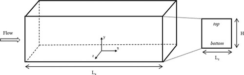
As mentioned previously, in order to investigate the effect of the dimples, a fully turbulent channel flow was considered. Channel flow is defined as a flow between two infinite parallel plates driven by a constant mean pressure gradient or mass flow rate. This provides a homogeneous flow in streamwise, $x,$ and spanwise, $z$, directions for smooth walls. From the computational framework, this structure allows the application of periodic boundary conditions in both directions. The computational domain and coordinate system used in the study are presented in Figure 1.

Figure 1. Computational domain and coordinate system of the fully turbulent channel flow.

As far as the studies involving dimpled surfaces in the literature are concerned (e.g. [7,10,17,19,26,27]), it can be clearly observed that the depth to diameter ratio, $d/D$, which is one of the fundamental parameters defining the dimples, is nearly concentrated on 0.015, 0.05, and 0.08. According to the information gained from the literature, four different depth to diameter ratios of 0.015, 0.03, 0.04 and 0.08 were selected for the examination. The diameters of the dimples, on the other hand, were determined by taking the physical dimensions of the measuring section of the flow channel, which is located at the University of Strathclyde, where the experimental tests are planned to be conducted. The dimensions of this facility’s rectangular measuring section are 598 mm$\times$180 mm$\times$22.5 mm [28]. Accordingly, dimple diameters of 22.5, 45 and 60 mm were chosen for the computational investigation to meet the physical dimensions of the experimental facility to allow future comparisons between the computational and experimental results. Concerning the coverage ratio, $CR$, of the dimples, which is another critical parameter, while van Nesselrooij et al. [10] mention that increasing $CR$ has a negative effect on drag reduction, there exist other studies in the literature that also point out a drag increase when the coverage ratio is less than 70% (e.g. [7,18]). In this study, it was decided to apply as high a coverage ratio as possible by considering the production tolerances in future experimental studies as well as real-life applications. Consequently, $CR$ was kept larger than 85% for all dimpled cases.

A staggered arrangement of the dimples was also considered in the study as it was found to be an advantageous geometric structure with a high drag reduction rate [10]. However, the initial calculations showed that this configuration further increased the skin friction and for the rest of the dimpled cases a flow-aligned arrangement was applied. On the other hand, a diamond-shaped dimple geometry was also used in the recent study of Ng et al. [19] and it was found to be highly effective and to have great drag-reducing potential. For this reason, it was decided to include this special type of dimple geometry in the present study in addition to the circular dimple types.

Besides the great potential of the dimples observed in the experimental studies, their real-life applications are also of critical importance in terms of applicability and cost-effectiveness. However, scientific publications about the real-life applications of dimples are rare in the open literature. The only example published in a German magazine [13] is about an application for high-speed trains which states a decrease in aerodynamic forces is around 17%. In the present study, the depth and diameter values of the dimples were selected aiming to represent a real-life marine application as far as possible by considering the constant channel height of the fully turbulent flow channels and the similarity of $d/\delta$ where $\delta$ represents the boundary layer thickness corresponding to the half channel height. As an example, by taking a 140 m tanker into consideration as a reference ship geometry, at the ship scale, a depth of 80 mm corresponds to a $d/D$ rate of 0.04 and $d/\delta$ rate of 0.15, which are comparable with a flow channel experiment.

A friction Reynolds number of $R{e}_{\tau }\cong 180$, which is based on the friction velocity, $u_{\tau }=\sqrt{{\tau }_w/\rho }$, and half channel height was considered in the computations where ${\tau }_w$ and $\rho$ specify streamwise wall shear stress and density, respectively. All values non-dimensionalised by $u_{\tau }$ are indicated with a superscript ${}^{+}$ throughout the paper. The Reynolds number based on the channel height and the mean bulk velocity, $R{e}_H,$ was nearly 5600 for all cases. The mean bulk velocity can be expressed as follows: (1) $U_b=\frac{1}{A}\int \int \text{U}(y,z)dydz$(1) where $A$ is the cross-section area at the inlet boundary and $U$ is the mean streamwise velocity.

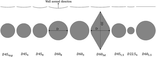
Table 1 lists the fundamental parameters selected for the computational cases along with the corresponding Reynolds numbers and grid resolutions. In the table $R{e}_D$ and $R{e}_d$ imply the Reynolds numbers based on $D$ and $d$, respectively. The profile and top views of the dimpled cases are shown in Figure 2.

Table 1. The cases investigated.

Case	$L_x/\delta$	$L_z/\delta$	D [mm]	d [mm]	$d/D$	$d/\delta$	$CR$ [%]	$R{e}_D$	$R{e}_d$	Total Cells	${\mathrm{\Delta }}_x^{+}$	${\mathrm{\Delta }}_z^{+}$
FP			–	–	–	–	–	–	–	3.50M
$D{45}_{4sg}$	13.86	4.00	45	1.800	0.040	0.04	91	11199	448	3.50M	11	11
$D{45}_8$	12.67	7.31	45	3.600	0.080	0.08	90	11196	896	5.84M
$D{45}_4$	12.67	7.31	45	1.800	0.040	0.04	90	11199	448	5.84M
$D{45}_{1.5}$	12.67	7.31	45	0.675	0.015	0.02	90	11200	168	5.84M
$D{60}_8$	17.07	9.85	60	4.800	0.080	0.11	88	14927	1194	10.60M
$D{60}_3$	17.07	9.85	60	1.800	0.030	0.04	88	14933	448	10.60M
$D{60}_{3d}$	13.86	4.00	60	1.800	0.030	0.04	89	14933	448	9.07M
$D{60}_{1.5}$	17.07	9.85	60	0.900	0.015	0.02	88	15146	227	5.80M

Figure 2. The side profiles (top) and top views (bottom) of the dimple geometries.

The dimensions of the computational domain involving solely flat surfaces were non-dimensionally defined as a cuboid with length ($L_x$), width ($L_z$) and channel height $(H)$ of $4.41\pi \delta ,1.27\pi \delta$ and $2\delta$, respectively, which corresponds to a rectangular domain size of 156 mm $\times$ 45 mm $\times$ 22.5 mm. The size of the computational domain was defined by considering the dimple dimensions. For each case, three and two dimples were placed in the streamwise and spanwise directions, respectively. Consequently, the dimension of the computational domain varied according to the dimple arrangements as presented in Table 1. The top wall was specified as a flat surface and the dimples were placed on the bottom wall. Circular dimples were described by the following depth function, $h$ [29]. (2) $h(x)=\left\{\begin{array}{ccc}0& ,x^2\ge {\displaystyle \frac{D^2}{4}}{\displaystyle \frac{D^2-4d^2}{8d}}-\sqrt{{\left({\displaystyle \frac{4d^2+D^2}{8d}}\right)}^2-x^2}& ,x^2<{\displaystyle \frac{D^2}{4}}\end{array}\right\},$(2) In the above equation, $x$ is the longitudinal location, and $d$ and $D$ are the dimple’s depth and print diameter, respectively.

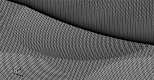
A structured mesh type was used for all computational cases. The grid spacing was kept constant in the streamwise and spanwise directions. In the vertical direction, a slowly growing mesh size up to a height level of $\delta$ was adopted whilst the $y^{+}$ value of the first grid in the immediate vicinity of the bottom surface, $\Delta y_w^{+}$, remained around 0.2. A view of the grid structure used for the dimpled cases can be seen in Figure 3.

Figure 3. An example of the grid structure used for the dimpled cases.

3. Methodology

Large Eddy Simulation (LES) was adopted as a scale-resolving approach to be able to get richer information about the flow with a high level of accuracy. We know that using LES is a proven approach to study complex flows in narrow channels [30,31]. The motion of a fluid is governed by the incompressible unsteady Navier-Stokes equations that can be expressed in Cartesian tensor form as follows: (3) $\begin{array}{rl}& \frac{\mathrm{\partial }{u}_i}{\mathrm{\partial }{x}_i}=0\end{array}$(3) (4) $\begin{array}{rl}& \rho \left(\frac{\mathrm{\partial }{u}_i}{\mathrm{\partial }t}+\frac{\mathrm{\partial }(u_i{u}_j)}{\mathrm{\partial }{x}_j}\right)=-\frac{\mathrm{\partial }p}{\mathrm{\partial }{x}_i}+\frac{\mathrm{\partial }}{\mathrm{\partial }{x}_j}\left(\mu \left(\frac{\mathrm{\partial }{u}_i}{\mathrm{\partial }{x}_j}+\frac{\mathrm{\partial }{u}_j}{\mathrm{\partial }{x}_i}\right)-{\tau }_{ij}\right)+F_i\end{array}$(4) where $\rho$, $\mu$, $u$ and $p$ represent fluid density, dynamic viscosity, space-filtered velocity and space-filtered static pressure, respectively. $F_i$ implies the mean streamwise forcing to create a fluid flow against friction. It is customary to impose a constant value for either the flow rate or the pressure gradient to create a fluid flow against friction. ${\tau }_{ij}$ is the anisotropic part of the stress tensor, which is also known as the subgrid-scale stress tensor. To compute the effect of this residual stress tensor, the Wall-Adapting Local Eddy-Viscosity (WALE) model of Nicoud and Ducros [32] was employed.

A finite-volume-discretisation-based solution algorithm was applied [33,34] to solve the equations. Implicit filtering was used for the filtration of the eddy scales that are smaller than the filter width or computational grid spacing used. The velocity-pressure coupling was achieved with the PISO method [35] which is a pressure-correction technique providing a relatively high convergence speed for time-dependent simulations. A second-order central differencing scheme was used for the viscous terms whilst a bounded central differencing scheme [36,37] was applied for the convective terms. The second-order implicit time-discretisation [38] was applied for unconditionally stable and accurate solutions. A double-precision solver was chosen for the computations. Convergence is achieved when the residuals of the equations reach a predetermined value. In each case, the inner iterations were run until the scaled residuals dropped to 10⁻⁵. In addition, after each iteration, the variation of the flow variables at various locations close to the bottom wall was checked. The iterations were continued until negligible differences were obtained between the results of two consecutive iterations. The simulations were carried out by using a widely known commercial code Star-CCM + .

A fixed mass flow rate was used for the streamwise periodicity at the inlet and outlet boundaries, and it was adjusted according to the changing cross-sectional areas between different cases to keep $U_b$ fixed for each case. Considering the constant mass flux in the channel $R{e}_H$ can be specified for the simulation.

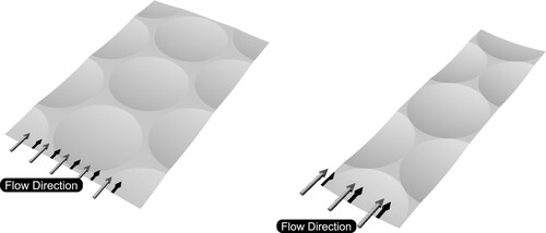
To trigger the small-scale fluctuations and to achieve a faster convergence in the computations, a synthetic turbulence field was specified inside the computational domain by using the turbulence intensity and length scale as the initial condition. In addition to the streamwise periodicity, the spanwise periodicity, which allows for avoiding the effects of the secondary flow near the channel corners and reduces the computational requirements, was also implemented at the side boundaries. No-slip boundary conditions were used at the flat top and dimpled bottom walls. The computational domain consisted of a cut-out of the channel according to the dimple diameter and alignment as sketched in Figure 4.

Figure 4. Flow-aligned configuration of dimples (left), the staggered configuration of dimples (right).

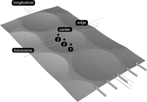
The collection of the node, surface and volume data was performed with different sampling rates due to the enormous memory and disk space requirements of the simulations. Eight straight lines were defined in streamwise and spanwise directions at four different heights. Each line allowed the collection of time-varying data for each cell along the lines. Two vertical line probes were located at the dimple centre and the dimple edge in the spanwise direction. The instantaneous wall shear stress values were collected at four different nodes, in the spanwise direction. The node data were recorded with a frequency of 1666 Hz. Likewise, the surface averaged drag and wall shear stress signals were gathered at the same frequency for the bottom wall. Four planes at different heights of $y^{+}=2,17,86\text{and}180$ were also defined parallel to the bottom wall to collect data with a sampling rate of 166 Hz including the bottom wall. Both node and surface data were recorded for 20 s. The data of the whole flow volume, on the other hand, were saved at a low sampling rate of 1/50 for 3 s. The locations where the data were collected can be seen in Figure 5. Considering the different geometry of the diamond-shaped case, an effective length, $D^{\ast }$, is used to define the longitudinal dimension of the dimples which is equal to D for the circular dimples and equal to 2D for the diamond-shaped dimpled case.

Figure 5. Data collection locations: Longitudinal (x) and transverse (z) beams represent the location of the data collection positions at different heights of ${\text{y}}^{+}=2,17,86$ and $180$. 1, 2 and 3 represent the data collection points in the longitudinal direction at $\text{x}/{\text{D}}^{\ast }=0.25,0.5$ and $0.75$, respectively.

4. Verification and validation

4.1. Flat plate cases

For verification and validation purposes, a series of fully turbulent channel flow simulations with different grid resolutions were performed. As the reference work, the DNS dataset of Moser et al. [24] was selected. The domain size and mesh resolution of the fully turbulent channel used in the mentioned DNS work are presented in Table 2.

Table 2. Domain size and mesh resolution of DNS dataset [24].

$R{e}_{\tau }$	$R{e}_H$	$L_x$	$L_z$	$N_x$	$N_y$	$N_z$	${\Delta }_x^{+}$	${\Delta }_z^{+}$	${\Delta }_{yc}^{+}$
180	5600	$4\pi \delta$	$4\pi \delta /3$	128	129	128	17.7	5.9	4.4

In the table, $N$ and ${\Delta }^{+}$ represents the number of cells and non-dimensional cell dimensions in the $x$, $y$ and $z$ directions, respectively. ${\mathrm{\Delta }}_{yc}^{+}$ is the cell height at the centreline of the channel in wall units. In line with the work of Moser et al. [24], the grid convergence study was carried out at $R{e}_{\tau }\approx 180$.

The grid dependency analysis was completed in two stages. In the first stage, the effect of the number of cells in the streamwise and spanwise directions on the results was investigated while keeping the total number of cells in the wall-normal direction constant. After the determination of the adequate resolution in the $x$ and $z$ directions, in the second stage, the mesh resolution was solely varied in the $y$ direction. The time step used in the grid dependency analysis was ${\mathrm{\Delta }}_t^{+}\approx 0.15$ which is non-dimensionalised by the $u_{\tau }$ and kinematic viscosity, $\nu$. 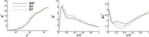The grid configurations used in the first stage of the verification study are listed in Table 3 along with the surface-averaged mean streamwise wall shear stress values, ${\overline{\tau }}_w$, obtained for each computational case. The comparison of the velocity, turbulent kinetic energy and shear stress profiles with those of the DNS work of Moser et al. [24] are also presented in Figure 6 for the three selected cases. It can be seen that for the resolution levels that are coarser than ${\mathrm{\Delta }}_x^{+}={\mathrm{\Delta }}_z^{+}=11$ the value of ${\tau }_w$ is highly variable. Consequently, by also taking the required simulation times and available computational resources into consideration, the resolution of the mesh configuration $FP5$ was found to be suitable and was selected for the rest of the simulations. It is concluded that the grid resolution of ${\mathrm{\Delta }}_x^{+}={\mathrm{\Delta }}_z^{+}=11$ is sufficient to obtain grid-independent Reynolds stresses based on the discussions of Piomelli et al. [39].

Table 3. Resolutions used in the first stage of the verification study.

Case	${\mathrm{\Delta }}_x^{+}$	${\mathrm{\Delta }}_z^{+}$	${\mathrm{\Delta }}_{yc}^{+}$	$\mathrm{\Delta }{y}_w^{+}$	$N_x$	$N_z$	$N_y$	Cell count	${\overline{\tau }}_w$[Pa]
$FP1$	50	50	79	0.2	58	17	128	$0.13\times {10}^6$	0.156
$FP2$	30	30	79	0.2	97	28	128	$0.35\times {10}^6$	0.191
$FP3$	18	18	79	0.2	162	47	128	$0.97\times {10}^6$	0.230
$FP4$	14	14	79	0.2	208	60	128	$1.61\times {10}^6$	0.241
$FP5$	11	11	79	0.2	265	77	128	$2.60\times {10}^6$	0.248
$FP6$	9	9	79	0.2	324	94	128	$3.89\times {10}^6$	0.251
$FP7$	7	7	79	0.2	417	120	128	$6.42\times {10}^6$	0.253

Figure 6. Comparison of the results of the different grid resolutions for the non-dimensional velocity (left), turbulent kinetic energy (mid) and shear stress (right) profiles.

As mentioned previously, in the second stage of the verification study, the subsequent simulations proceeded by varying the grid spacing in the $y$ direction. The resolution in the other directions remained unchanged. The configurations applied for the second stage of the grid dependency analysis for each case are shown in Table 4. As is seen, the value of ${\overline{\tau }}_w$ did not display any variation with the application of the incremental grid resolution. However, further examinations showed that $FP5\mathrm{f}$ provides better accuracy in terms of velocity, $u^{+}$, turbulent kinetic energy, $k^{+}$, and shear stress, ${\overline{uv}}^{+}$, profiles displaying closer results to the finest grid structure $FP7$ as can be seen in the comparative plots presented in Figure 6. The plots particularly indicate that $FP5\mathrm{f}$ is capable of better capturing the peak level of $k^{+}$ and ${\overline{uv}}^{+}$. Accordingly, it was decided to proceed with $FP5\mathrm{f}$ for the subsequent analyses. The grid includes 9 points below $y^{+}=5$ and 18 points below $y^{+}=10$, satisfying the requirement of having at least 10 grid points within the first 9 wall units for accurate resolution of near-wall flow physics [40].

Table 4. Configurations for the Y grid spacing.

Case	${\mathrm{\Delta }}_x^{+}$	${\mathrm{\Delta }}_z^{+}$	${\mathrm{\Delta }}_{yc}^{+}$	$\mathrm{\Delta }{y}_w^{+}$	$N_x$	$N_z$	$N_y$	Cell count	${\overline{\tau }}_w$ [Pa]
$FP5$	11	11	79	0.2	265	77	128	$2.60\times {10}^6$	0.248
$FP5\mathrm{f}$	11	11	56	0.2	265	77	172	$3.50\times {10}^6$	0.248
$FP5\mathrm{c}$	11	11	112	0.2	265	77	94	$1.91\times {10}^6$	0.247

Furthermore, to capture the effect of the time step on the results additional simulations with smaller time steps were also conducted. The application of the non-dimensional time steps of 0.07 and 0.28 showed no appreciable variations in the results, however, substantially increased the computational time. Consequently, the rest of the simulations proceeded with ${\mathrm{\Delta }}_t^{+}\approx 0.15$.

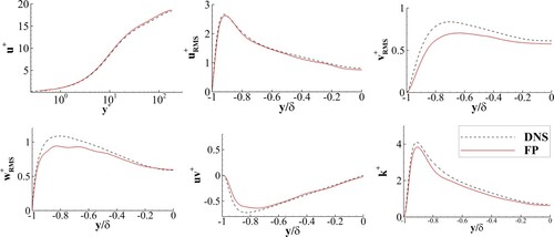
In Figure 7, the profiles of the streamwise mean velocity, fluctuating RMS velocity components, shear stress and turbulent kinetic energy, TKE, obtained from the present LES study are comparatively presented along with those of the DNS work of Moser et al. [24]. All values are non dimensionalised by using $u_{\tau }$. A good agreement was generally found in all profiles. Particularly, the streamwise mean and RMS velocity profiles closely follow the DNS data. The transverse and vertical components of the RMS velocities slightly underestimate the DNS values; however, the trend of the profiles indicates a good correlation, and the results were found satisfactory. Likewise, the agreement of the shear stress and turbulent kinetic energy profiles is good. Considering the compatibility with DNS data, it was decided that the grid resolution selected would be appropriate to be used in the present study.

Figure 7. Comparison of the $FP$ case with the DNS results.

4.2. Dimpled cases

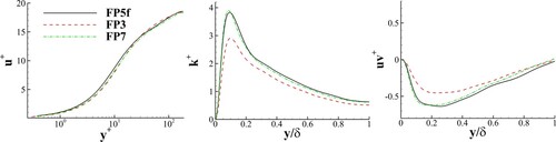
The same systematic approach was followed for the verification of the grid structures generated for the dimpled cases. The exact grid resolutions were applied to the dimpled case $D{45}_{4sg}$, which was selected for this grid convergence study. The configurations used in the first stage of the verification study are presented in Table 5 along with the ${\overline{\tau }}_w$ value obtained for each computational case. A good convergence can be detected following $D5$ which has a resolution of ${\mathrm{\Delta }}_x^{+}={\mathrm{\Delta }}_z^{+}=11$. Consequently, for the second stage of the grid convergence study, $D5$ was selected. The configurations applied for the second stage of the grid dependency analysis for each case can be observed in Table 6. The comparative profiles of velocity, turbulent kinetic energy and shear stress are also presented in Figure 8. The results showed that the application of $D5\mathrm{f}$ significantly increases the accuracy of the profiles and was selected to be used for the rest of the dimpled simulations.

Table 5. Resolutions used in the first stage of the verification study for the dimpled cases

Case	${\mathrm{\Delta }}_x^{+}$	${\mathrm{\Delta }}_z^{+}$	${\mathrm{\Delta }}_{yc}^{+}$	$\mathrm{\Delta }{y}_w^{+}$	$N_x$	$N_z$	$N_y$	Cell count	${\overline{\tau }}_w$ [Pa]
$D1$	45	45	79	0.2	65	19	128	$0.16\times {10}^6$	0.193
$D2$	30	30	79	0.2	97	28	128	$0.35\times {10}^6$	0.227
$D3$	18	18	79	0.2	162	47	128	$0.97\times {10}^6$	0.258
$D4$	14	14	79	0.2	208	60	128	$1.61\times {10}^6$	0.269
$D5$	11	11	79	0.2	265	77	128	$2.60\times {10}^6$	0.278
$D6$	9	9	79	0.2	324	94	128	$3.89\times {10}^6$	0.279
$D7$	7	7	79	0.2	417	120	128	$6.42\times {10}^6$	0.280

Table 6. Configurations for the Y grid spacing for the dimpled cases.

Case	${\mathrm{\Delta }}_x^{+}$	${\mathrm{\Delta }}_z^{+}$	${\mathrm{\Delta }}_{yc}^{+}$	$\mathrm{\Delta }{y}_w^{+}$	$N_x$	$N_z$	$N_y$	Cell count	${\overline{\tau }}_w$ [Pa]
$D5$	11	11	79	0.2	265	77	128	$2.60\times {10}^6$	0.278
$D5\mathrm{f}$	11	11	56	0.2	265	77	172	$3.50\times {10}^6$	0.276
$D5\mathrm{c}$	11	11	112	0.25	265	77	94	$1.91\times {10}^6$	0.275

Figure 8. Comparison of the results of the different grid resolutions for the non-dimensional velocity (left), turbulent kinetic energy (mid) and shear stress (right) profiles.

5. Results and discussion

5.1. Drag characteristics

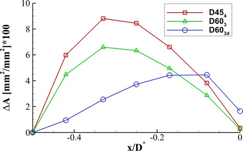
The left plot in Figure 9 shows the reduction obtained in the frictional component of the total drag force acting on the dimpled surfaces, which is related to the streamwise component of the wall shear stress. At this point, it should be recalled that the potential positive effect of the dimples is related to the skin friction component of the total drag force. However, they naturally generate a form drag component, which represents the streamwise component of the viscous pressure force that can be calculated by the difference between the total drag and skin friction force. When the amount of the gain in the skin friction component exceeds the amount of the loss in the form drag component as form drag increases, the total drag force can be reduced. It is seen that most of the dimpled surfaces positively affected the skin friction and effectively reduced it with respect to that of $FP$. The larger dimpled cases with a diameter of 60 mm generally displayed better performance in terms of friction, probably due to the higher Reynolds number seen by the flow inside the dimples with the exception of $D{60}_8$. This case along with $D{45}_{4sg}$, which was organised with a staggered arrangement, increased the surface friction. The plot points out that, taking solely the frictional performance into account, the optimal dimpled depth is around 3-4%, which resulted in the maximum friction reduction of 2% and 4% for both dimple diameters (of 45 and 60 mm) considered, respectively. The tests with larger or smaller dimpled depths gave lower reduction rates. The diamond-shaped $D{60}_{3d}$, on the other hand, exhibited a successful skin friction performance with a significant reduction rate of 4.9%.

Figure 9. Friction and total drag reduction percentages for each computational case (The percentages were calculated with respect to the reference value of $0.248$ Pa obtained for $FP$. The negative values indicate an increase in the drag component).

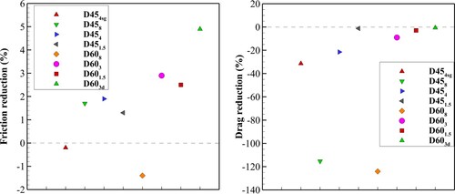
The right plot in Figure 9 displays the total drag force reduction rates obtained from the dimpled cases. As is seen, no case achieved a reduction in drag force due to the additional form drag component that is generated by the dimples. Most of the dimpled cases substantially increased the total drag acting on the bottom surface. However, the two most shallower cases ($D{45}_{1.5}$ and $D{60}_{1.5}$) along with $D{60}_{3d}$ produced an encouraging outcome displaying almost no increase in drag, indicating that further studies with a slight optimisation in the dimple geometry will likely result in a considerable drag reduction.

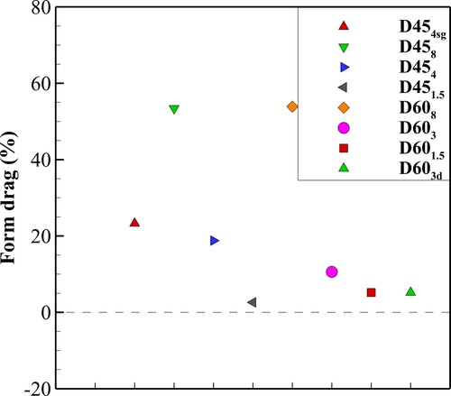
The ratio of the contribution of the form drag component to the total drag force is given in Figure 10 for different cases. It is clear that the application of deeper dimples should be avoided due to their enormous profile drag. The plot shows that the depth of the dimples should be at most 3%, while, in fact, this configuration also displays a considerable form drag rate of 10%. The implementation of larger depths substantially increases the additional contribution of the form drag. The staggered arrangement also resulted in a very high rate of above 20%. On the other hand, although a depth of 3% was applied to the diamond shaped dimples, the form drag rate of this arrangement was not found to be higher than that of the shallower dimpled case $D{60}_{1.5}$. The study reveals, then, the great potential of this configuration which exhibited a significant skin friction reduction and a relatively low form drag rate.

Figure 10. Percentages of the contribution of the form drag to the total drag for each computational case.

5.2. Time-averaged and fluctuating flow fields

In the following sections, the comparative flow fields of the selected cases are presented for brevity. The cases with a $d/D$ rate of 0.08 are avoided since they presented an entirely different flow structure with significant flow separation. The staggered arrangement was also not decided as the general focus of the study is on flow-aligned arrangements. To provide a clearer representation of the differences with respect to the skin friction reduction performance the two best performing computational cases, $D{60}_3$ and $D{60}_{3d}$, and the case with the lowest reduction rate amongst the rest, $D{45}_4$ alongside $FP$ were selected for further investigation.

The mean (time-averaged) flow fields were obtained from the temporally averaged velocity and stress distributions for all cases. The mean streamwise wall shear stress, ${\overline{\tau }}_w$, distributions non-dimensionalised by the surface-averaged ${\overline{\tau }}_w$ of the $FP$, ${\overline{\tau }}_w^{FP}$, on the bottom wall along with the limiting streamline traces can be examined in Figure 11. As expected, $FP$ displays a nearly homogenous stress distribution throughout the surface while the stress values were found to be around 1.02. The circular dimpled cases present rounded contour shapes around the entrance of the dimples with a large gradient along with them. Due to its highest streamline curvatures, the largest gradient in the wall shear stress was observed in $D{45}_4$ where very low-stress values of below 0.041 were computed around the leading edge of the dimples. Flow separation and reattachment within the dimple can be observed for $D{45}_4$. A closer observation in $z=0$ cross-sectional plane, which is not presented here for brevity, indicated that the separation is limited to a zone in the immediate vicinity of the wall. The recirculation further helps decrease the streamwise wall shear stress around this zone. One can see from the plots that the introduction of the dimples generates substantial transverse flow motion. Due to the existence of the separation zone, the flow largely moves towards the outer edges of the dimple and the streamline traces becomes sparse following the separation for $D{45}_4$. The zig-zag nature of the flow can also be seen in $D{60}_{3d}$ where a smoother distribution of the stream traces covers the dimpled wall. One can see that the structure of the streamlines is rather different from that of the circular dimpled cases. The sudden deflection of the streamline following the boundaries of the dimples is striking. Near the leading edge, the strong convergence of the streamlines can be also observed while they diverge towards the trailing edges. The stress values progressively raised along with the dimples up to the trailing edges where the largest stress values of over 2.03 were obtained. An identical stress structure was predicted for $D{60}_3$ where the maximum and minimum values were computed as 0.16 and 2.85, respectively. The flat zones remaining between the dimples exhibited stress values generally larger than those of $FP$. The case that displayed the best skin friction performance, $D{60}_{3d}$, on the other hand, presented a more uniform stress distribution through the surface, where the values on a large portion were found to be below those of $FP$. The largest values of around 1.63, which are higher than those of $FP$ but are rather lower than those of the other two cases presented, occurred in a confined space near the trailing edges of the dimples.

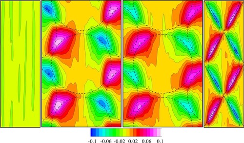
Figure 11. ${\overline{\tau }}_{\text{w}}/{\overline{\tau }}_{\text{w}}^{\text{FP}}$ distributions and limiting streamlines on the bottom wall ($\text{FP}$, $\text{D}{45}_4$, $\text{D}{60}_3$, $\text{D}{60}_{3\text{d}}$, from left to right, respectively. The flow is from bottom to top.).

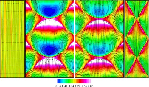
Figure 12. Velocity vectors and ${\overline{\tau }}_w/{\overline{\tau }}_w^{FP}$ on the centre plane along the longitudinal centre plane of the dimples (from top to bottom $FP$, $D{45}_4$, $D{60}_3$, $D{60}_{3d}$, respectively).

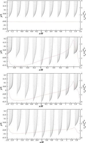
Figure 13. Pressure Coefficient distributions on mid dimple centred area on surface ($FP$, $D{45}_4$, $D{60}_3$, $D{60}_{3d}$, from left to right, respectively. The flow is from bottom to top.).

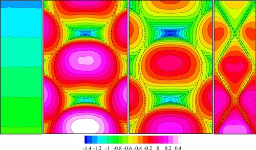
Figure 14. Sectional area variations for dimpled cases.

The velocity vectors and the non-dimensional profiles of ${\overline{\tau }}_w$ along the longitudinal centre plane of the bottom surface are shown in Figure 12 for the computational cases considered. As can be seen and expected, in the near wall region, inside a dimple, the gradients of the tangential velocities in the vertical direction and the streamwise component of wall shear stresses are related to each other. The incompressible flow in the channel exhibits a diffusion and contraction-like behaviour in the vertical direction as it passes through a dimple. The large wall shear stress gradient exhibited by the two circular dimpled cases particularly around the last quarter of the dimples is immediately striking in the figure. As can be observed, when a portion of the flow near the bottom wall moves towards the dimple, the boundary layer becomes somewhat stretched while the displacement thickness remains almost constant. In this way, the expansion area provided by the dimple causes the fluid flow to slow down and the velocity gradients to decrease, leading to a reduction in the streamwise wall shear stresses. This fluid flow also increases the local pressure due to the reduced velocity magnitude. Figure 13, which shows the pressure distribution on the bottom wall, can be examined along with Figure 12. For the circular dimpled cases, it can be seen that approximately after the first quarter of the dimple, the velocity gradients begin to rise while the fluid flow remains inward. The change in the direction of the flow severely increases the wall shear stress levels approaching to the trailing edge of the dimples due to the contraction trend of the surface geometry where the velocity levels increase and pressure levels drop. However, the pressure drop rate around the second half of the circular dimples appears to be shifted towards the trailing edge of the dimples and the pressure distribution displays an asymmetrical structure with respect to the spanwise axis of the dimple. This is due to the high velocity flow around the outer region of the boundary layer which is barely directed inward as the flow reaches the centre of the dimple, where the dimple geometry starts to get shallower. As the fluid continues to flow forward, the geometry of the surface forces the flow to change its direction and to move upward, leading to a stagnation pressure and an increase in the velocity level in the near wall region. This also explains the sudden increase in wall shear stresses at that zone. Additionally, the high-pressure region on the dimple wall shifts towards the trailing edge, contributing to the pressure-induced drag. As mentioned previously, an asymmetrical nature of the flow can be examined for the circular dimpled case in Figure 12 in terms of the vertical velocities. The accelerated upward flow near the trailing edge of the dimples enhances the tangential velocity on the surface and hence the friction force in that area. As seen in the figure the tangential velocities and the velocity gradient become relatively large towards the trailing edge of the dimple for the two circular dimpled cases. From this perspective, it could be argued that increasing the length of the dimple without changing the depth and width would decrease the harsh slope at the leading and trailing edges and potentially reduce the vorticity, pressure difference, and therefore the form and frictional drag. This may explain the reason for the lower drag components predicted for the diamond-shaped dimpled case which presents an almost symmetrical flow structure around the spanwise axis of the dimple and slowly rising walls shear stress levels. This is simply related to the geometric specifications of the dimpled walls. The circular dimples have a parabolic change in their sectional area with a rapid increase and rapid decrease at the leading and trailing edges, respectively. However, the diamond-shaped dimple exhibits a more linear variation. The sectional area variation rates normalised by the projection area of the dimples for the cases considered are shown in Figure 14. The variation of the sectional area at the edges is highest for the $D{45}_4$ case and lowest for the $D{60}_{3d}$ case, due to its wedge-like shape, which reflects the performance of the surfaces in the skin frictional reduction. A comparison of Figure 11 and Figure 14 reveals an inverse relationship between sectional area variation rates and wall shear stresses. Indeed, there should be an optimal dimple length depending on the bulk velocity, boundary layer thickness, etc. Obviously, an infinitely long dimple would not be effective on the drag reduction. However, an excessively shorter length would increase the frictional and form drag due to the arguments explained above.

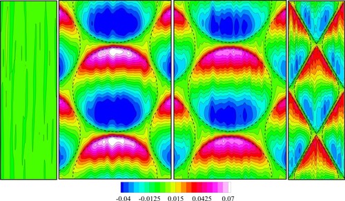
The vertical non-dimensional mean velocity fields are presented in Figure 15. As explained previously, due to the bottom surface geometry the flow is forced to display a diffusion and contraction-like behaviour, which indeed generates vertical velocity components. The vertical velocities tend to increase or decrease parallel to the ascending or descending surface profiles. However, they display an asymmetrical structure with respect to the spanwise axis of the dimples, which does not reflect the exact geometry of the dimple surfaces. An interesting resemblance of the vertical velocity distributions to those of the streamwise wall shear stress fields is remarkable. This particularly enhances the previously explained physical mechanism involving the relationship between the structure of the flow, skin friction, and wall pressure levels. $FP$ displays a nearly zero vertical velocity level through the flow field as expected whilst $D{45}_4$ presents the largest velocity gradient in the streamwise direction due to the stronger curvature of the dimple profiles as indicated previously. A much smoother contour structure can be observed in the diamond-shaped dimpled case. The figure highlights the relationship between the smoother surface profiles and the frictional resistance. A slight variation in the surface depth is enough to create the vertical motion and substantially modify the boundary layer and the velocity gradients. This encourages the optimisation studies to take the variation of the sectional area of the dimples into consideration to create substantial friction reduction without largely increasing the form drag component.

Figure 15. Vertical non-dimensional mean velocity ($V/U_b$) distributions at $y^{\ast }/H=0.05$ ($FP$, $D{45}_4$, $D{60}_3$, $D{60}_{3d}$, from left to right, respectively. The flow is from bottom to top.).

The streamwise non-dimensional mean velocity distributions at a height of $y^{\ast }/H=0.05$ are presented in Figure 16 for different computational cases. The velocity values were normalised by the associated bulk velocities. Here, $y^{\ast }$ represents the distance from the flat sections of the bottom surface where zero depth is defined. It should be noted that the $y^{+}$ values are not constant through that plane due to the changing distance from the bottom surface of the dimples and varying local wall shear stress values. At $y^{\ast }/H=0.05$, the $y^{+}$ values are around 17 on the zones corresponding to the areas between the dimple geometries and the sides of the dimple structure. The $y^{+}$ values are rising to 45 along the front half of the dimple geometry and fall to 1 along the aft half for $D{45}_4$. The maximum value tends to stay around 45 while the minimum value increases with the increasing wall shear stress up to 17 for the $D{60}_{3d}$.

Figure 16. Streamwise non-dimensional mean velocity ($U/U_b$) distributions at $y^{\ast }/H=0.05$ (FP, $D{45}_4$, $D{60}_3$, $D{60}_{3d}$, from left to right, respectively. The flow is from bottom to top.).

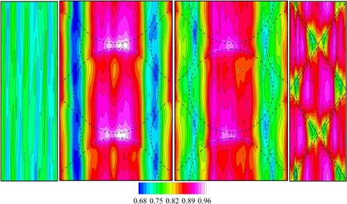
Concerning Figure 16, it is seen that $FP$ has a uniform distribution as expected. The dimpled cases present a nearly symmetrical structure about the dimple centreline. The two circular dimpled cases displayed high and low-velocity streaks on either side of the centreline. Due to the large velocity gradient found in the spanwise direction, it is expected to have counter-rotating pairs of streamwise vortices along the surface depending on the direction of the spanwise velocity component. The enhancing effect of the dimples on the vortex structures is also indicated by many research studies found in the related literature [5,14,15]. It can be seen that the relatively deeper dimpled case, $D{45}_4$, displays the largest peak velocity values and hence a larger velocity gradient highlighting the effect of $d/D$ on the flow field. For both circular dimpled cases, the highest streamwise velocity occurred between the consecutive dimple structures. Towards the side edges of the dimples, the lowest velocity levels were detected. The non-dimensional averaged velocity value for both cases was predicted as 0.83 and 0.85 respectively. For the diamond-shaped case, $D{60}_{3d}$, no continuous velocity streaks were observed about the centreline due to the tighter arrangement of the dimples. This dimpled case presented the highest velocity distribution among the cases investigated with a non-dimensional average velocity value of 0.87. Within a dimple structure, two high-velocity zones took place on either side of the centreline which were then followed by small low-velocity areas where the values were around those of $FP$. The occurrence of counter-rotating pairs of streamwise vortices seems to be likewise highly likely in that computational case, weaker vortices are nevertheless expected. The correlation between the streamwise velocity levels and the skin friction values of the different cases was found to be remarkable at this stage.

As far as the non-dimensional spanwise velocity distribution are concerned, in Figure 17, $FP$ presents almost no spanwise component which is quite expected. However, it can be clearly seen that the dimple structures induce significant spanwise components to the mean flow field as indicated, for instance, by Tay et al. [7], van Nesselrooij et al. [10] and Wang et al. [29]. The topology is largely dominated by the alternating spanwise flow. For the two circular dimpled cases, the peak values occurred in a relatively large zone between three adjacent dimple structures near the diagonal edges of the dimples due to the curvature of the streamline associated with the rounded shape of the dimples while the central zone of the dimples showed almost no spanwise component. The diamond-shaped dimples yet created strong spanwise components in a relatively more confined diagonal zone along the dimple edges. The peak values also occurred nearly on these edges. The information gained from the two velocity components investigated so far suggests an alternating arrangement of counter-rotating streamwise vortex pairs.

Figure 17. Transverse non-dimensional mean velocity (W$/U_b$) distributions at $y^{\ast }/H=0.05$ (FP, $D{45}_4$, $D{60}_3$, $D{60}_{3d}$, from left to right, respectively. The flow is from bottom to top.).

Investigating the flow topology given in Figures 16 and 17 in common, it can be deduced that another effect that may influence the high wall shear stress 1levels may be partly related to the spanwise motion of the flow. As seen in the figures, the spanwise component of the motion does not affect the whole surface area of the dimples. This flow structure is strongly related to the geometric arrangement of the dimples. In the flow-aligned arrangement, for the two circular dimpled cases, since a flow portion that leaves one dimple in the diagonal direction enters the adjacent one in the same direction, a zig-zag nature of the flow is generated around the edges of the dimples which are diagonally positioned. This flow portion cannot reach the middle of the dimples. Around the streamwise axis of the dimples, on the other hand, the flow displays higher velocity levels since the bottom wall surface is located at a deeper level. This flow gains a substantial acceleration passing through the area between two consecutive dimples in the streamwise direction. In this way, around this zone, high momentum levels are added to the inner part of the boundary layer and the shear stresses present a significant increase. This can be also observed in Figure 11 where the mean streamwise wall shear stress distributions are presented. The diamond shaped dimpled case, on the other hand, provides a somewhat stronger spanwise flow component which can affect the regions towards the middle of the dimple which relatively avoids the high-velocity streaks in the middle part of the dimple. This partly contributes to the lower wall shear stress values predicted around the trailing edges of the dimples.

The examination of the time-averaged flow fields so far basically reveals that the main effective influence on the surface friction originated from the mean flow. Based on the current research and existing literature, two physical mechanisms that are effective on the frictional drag reduction in the streamwise direction may be identified. The first one is the amount of gradient of the tangential velocities in the inner part of the boundary layer at the immediate vicinity of the bottom wall. This is directly related to the geometrical characteristics, particularly the sectional area variation rates of the bottom wall. Indeed, lower gradient values will decrease the overall amount of wall shear stresses. The second physical property, which is relatively effective on the frictional resistance, is the flow direction in high-speed regions close to the wall. If a high-momentum flow portion can be orientated to the spanwise direction, even if high shear stress levels exist on the fluid adjacent to the wall, a part of them will be transferred to the spanwise flow component, which is insignificant in terms of the skin friction resistance.

Shown in Figure 18 are the streamwise vorticity, ${\overline{\omega }}_x,$ distributions non-dimensionalised by $U_b$ and $H$ on the plane $y^{\ast }/H=0.05$. In the open literature, there is a quite solid belief that the dimple structures create strong streamwise vortices and there is a correlation between the relative depth of the dimples and the level of the vorticity or the size of the instantaneous vortices [7,15,41]. In addition, the related literature states that there exists a relationship between the size and/or level of these streamwise vortices and the skin friction reduction degree of the related dimple arrangement. Bearing these recommendations in mind, one can see in Figure 18 that $FP$ exhibits almost no streamwise vorticity with an occasional low level of positive component probably due to the need for a further long time-averaging period. However, with the introduction of the dimples, strong counter-rotating pairs of alternating streamwise vortex zones can be observed along the two corridors between the dimples for the two circular dimpled cases. The inner part of the dimples also displays a sparse zone of high-level vorticity. The level of the vorticity and the size of the affected area is the largest for $D{45}_4$ which has a relatively deeper dimple structure but the lowest skin friction reduction performance. $D{60}_{3d}$, presented a similar flow structure in terms of streamwise vorticity with quasi organised vortices along the edges of the dimples. The level of the vorticity and the size of the affected area were predicted to be lower than those of the two other dimpled cases whilst the best skin friction performance was found for this computational case. This suggests that the physical mechanism that lies behind the skin friction reduction performance of the dimples is not directly proportional to the introduction of the streamwise vortex structures at least without taking the generation of the spanwise vortices into account.

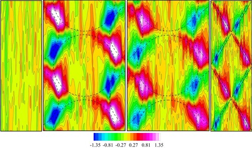
Figure 18. Streamwise non-dimensional mean vorticity (${\overline{\omega }}_x\times H/U_b$) distributions at $y^{\ast }/H=0.05$ ($FP$, $D{45}_4$, $D{60}_3$, $D{60}_{3d}$, from left to right, respectively. The flow is from bottom to top.).

The mean distribution of the non-dimensional spanwise vorticity (${\overline{\omega }}_z\times H/U_b$) at the vertical plane, $z/H=0$, passing through the longitudinal centre of the dimples can be seen in Figure 19. The figure indicates that $FP$ has a tendency for clockwise rotational motion around the spanwise axis due to the interaction between the streamwise and wall-normal fluctuations. The figure implies that the size of the high-level vorticity zones significantly increases with the introduction of circular dimples. It should be recalled that, at the zones where the spanwise vorticities are strong, the velocity gradients in the vertical and streamwise directions should present high levels. At these zones, hence, the instability of the flow should also be high. High levels of spanwise vorticity that are close to the wall would cause an increase in the frictional resistance about these zones. In the figure, it can be seen that for the two circular dimpled cases, the clockwise high-vorticity bands are slenderised in the zones between the dimples and near the trailing edges, but their intensity is increased. The figure shows that, around the leading edge of the dimple, the fluid with high-vorticity flows away from the bottom surface without affecting the wall shear stresses. The related zones correspond to those which display a substantial decrease in the skin friction pointed out previously. The diamond-shaped dimpled case, on the other hand, displays a much smoother flow structure. Around the leading edge, the relatively strong band remains closer to the wall without, however, presenting significantly high levels. The zones between the dimples and near the trailing edges, similarly, do not show extreme vorticity values. In this way, $D{60}_{3d}$ presented the most favourable skin friction performance. Table 7 shows the values of the spanwise non-dimensional mean vorticity computed at the immediate vicinity of the wall along the streamwise centre axis of the surface. As pointed out above, the considerable increments in the vorticity towards the trailing edge of the dimples for the two circular dimpled cases are remarkable in the table, whilst the variation of the values is seen as limited for $D{60}_{3d}$.

Figure 19. Spanwise non-dimensional mean vorticity distributions (${\overline{\omega }}_z\times H/U_b$) at $z/H=0$ ($FP$, $D{45}_4$, $D{60}_3$, $D{60}_{3d}$, from top to bottom, respectively. The flow is from left to right.).

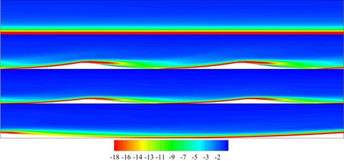
Table 7. Spanwise non-dimensional mean vorticity (${\overline{\omega }}_z\times H/U_b$) values at the vicinity of the bottom wall ($z/H=0$).

$X/D$	$FP$	$D{45}_4$	$D{60}_3$	$D{60}_{3d}$
$-0.50$	$\sim$22.5	40.9	34.7	25.1
$-0.25$	$\sim$22.5	1.6	5.1	14.9
$+0.00$	$\sim$22.5	17.3	19.9	19.6
$+0.25$	$\sim$22.5	37.4	29.2	23.2
$+0.50$	$\sim$22.5	74.3	56.0	29.5

To provide a better understanding of the underlying dynamics of the spanwise vorticity distributions, Figure 20 presents the instantaneous spanwise non-dimensional vorticity distributions (${\omega }_z\times H/U_b$) at an $xy$ plane passing through the dimple centrelines ($z/H=0$) at two different flow instants. The frames, which are captured with a rate of roughly 33 Hz, contain a single dimple structure for the dimpled cases with a display height of around $y^{\ast }/H=0.2$. The flow is from left to right. The structure of the vorticity and the effect of the dimples can be clearly investigated in the figures. In $FP$ Accumulation of the negative vorticity generates a shedding-like flow motion with an elongated vortex structure expanding slightly in the positive $y$ direction while losing its strength. The vortex shedding phenomenon is pronounced in the dimpled cases. The build-up of the high-level vorticity begins at the entrance of the dimple, due to the high curvature of the bottom surface and, hence, the limiting streamlines, mostly for the two circular dimpled cases. For the relatively deeper dimpled case, $D{45}_4$, the shedding is more visible. By closely examining the consecutive images, the breakdown of the high-strength vortex structure into smaller and weaker fluctuating vortices and the shedding into the flow field in the streamwise direction can be observed. A second vortex shedding phenomenon occurs around the centre of the dimple in a rapidly diminishing manner. The existence of the relatively deeper dimple structures clearly augments the spanwise vorticity traffic in the vicinity of the wall up to mostly $y^{\ast }/H=0.1$. A similar flow structure was computed for $D{60}_3$ which exhibited more elongated vortex zones with weaker strength. The fact that the strong vorticity band leaves the surface at the trailing edge and moves towards the bottom surface with a breakdown around the middle of the dimple while increasing its strength in a more confined zone may be explained by the directional change of the flow which leads to a stagnation pressure as pointed out previously.

Figure 20. Instantaneous spanwise non-dimensional vorticity (${\omega }_z\times H/U_b$) at centre plane ($z/H=0$) for different cases, $t_0=4.0s$ (top) and $\mathrm{\Delta }t=0.03s$. The flow is from left to right.

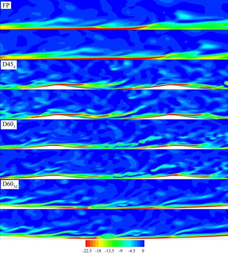
$D{60}_{3d}$, on the other hand, display relatively high vorticity levels and structures only in very slender zones closer to the wall compared to $FP$ and seemed to not increase the level of negative vorticity and diminish the turbulent exchange. Although the vorticity zones are distributed in a more frequent form, it can be observed that they are more diffused with generally lower values which agrees with its lower skin frictional performance.

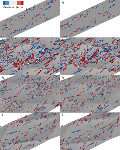
Shown in Figure 21 are the instantaneous $Q$ criterion [42] iso surfaces at different instants for the four computational cases examined. $Q$ values of $1000$ were selected to provide a readable graphical view. The top and bottom plots represent the iso surfaces coloured by streamwise and spanwise vorticity levels, respectively. It should be recalled that a vortex structure and vorticity have different physical meanings. For instance, a longitudinal structure does not necessarily contain solely streamwise vorticity or a spanwise structure can have both streamwise and spanwise vorticity components. The figures offer a clearer representation of the vortex structures near the bottom surface throughout the flow field. The figures indicate that $FP$ has discrete structures randomly spread in particularly streamwise directions. However, by close examination of the colours, one can foresee that the flow is mainly dominated by the spanwise vorticities. The left and right plots also demonstrate the motion of the structures over the period. The interaction of the structures with each other appears to be relatively low. The number of vortex structures significantly rises with the application of the dimples. In the two circular dimpled cases, the vortex structures spread in both streamwise and spanwise directions. However, they are once again under the influence of spanwise vorticities. The trailing edges of the dimples appear to be typically covered by spanwise structures. The discrete vortex formation mainly occurs inside the dimple close to the central location. The interaction between the discrete structures appears to be augmented particularly around the dimple centre. The diamond-shaped dimples show relatively similar behaviour to that of $FP$ producing much fewer vortex structures compared to the other two dimpled surfaces. A more uniform distribution over the surface can be observed throughout the surface. Whilst the number of the small-scale structures is higher than that of $FP$, they are generally in the streamwise direction. At this point, it should be noted that the critical aspect is the directional position of the small-scale structures rather than their quantity of rate of occurrence. Streamwise structures may not be significantly effective on the fictional resistance. However, spanwise structures located close to the wall surfaces have a much more negative influence on the skin friction performance, which are seen intensively around trailing edges of circular dimples.

5.3. Turbulent kinetic energy budget and spectral characteristics

In this section, we examine the turbulent kinetic energy budget and the spectral content of the velocity signals collected from different computational cases to reveal the effect of the dimples on the fluctuating energy levels of the time-dependent data and the turbulent kinetic energy (TKE) transport. The same computational cases, which were investigated in the previous sections, were considered.

Figure 21. Instantaneous $Q$ criterion iso surfaces ($Q=1000s^{-2}$) for $FP$, $D{45}_4$, $D{60}_3$, $D{60}_{3d}$, from top to bottom, respectively. Coloured by streamwise vorticity, $t_0=4.00s$ (left) and $t_1=4.03s$ (right).

In fluid dynamics, the term ‘turbulent kinetic energy budget’ refers to the balance of energy in a turbulent flow. In a turbulent flow, TKE is constantly being transferred from the large-scale motion of the fluid to the smaller-scale eddies and vortices that make up the turbulent flow. This transfer of energy is a critical factor in determining the overall behaviour of the turbulent flow. For the present channel flow, the turbulent kinetic energy transport equation can be written in Cartesian tensor notation as: (5) $-\overline{u_i{u}_j}\frac{\mathrm{\partial }\overline{u_i}}{\mathrm{\partial }{x}_j}-\nu \overline{\frac{\mathrm{\partial }{u}_i}{\mathrm{\partial }{x}_j}\frac{\mathrm{\partial }{u}_i}{\mathrm{\partial }{x}_j}}+\nu \frac{d^2}{d{y}^2}\left(\frac{1}{2}\overline{uu}\right)-\frac{d}{dy}\frac{1}{2}\overline{vuu}-\frac{1}{\rho }\frac{d}{dy}\overline{v{p}^{\mathrm{\prime }}}=0$(5) where the overbars indicate time averaging. This equation implies the balance of production ($P$), dissipation ($\epsilon$), viscous diffusion (VD), turbulent transport (TT), and pressure gradient (PG), respectively [43]. Figure 22 presents a comparison of the TKE budget terms for dimpled and flat channel flows obtained by the current LES study. The profiles at the dimple centre ($x/D=0$) are plotted against $y^{+}$ on the horizontal axis, which is the non-dimensionalised distance from the wall. The shear stress value used to estimate $y^{+}$ in these plots is the streamwise component of the mean wall shear stress of the bottom wall.

Figure 22. Comparative TKE budget profiles for the centre of the dimple.

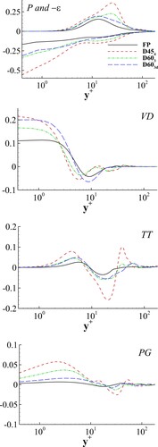
In Figure 22, it is clear that the introduction of the dimples significantly affects the turbulent kinetic energy transport phenomenon. An increase in the turbulence production can be observed for the dimpled cases within the range covering the viscous sublayer, buffer and logarithmic layer compared to that of $FP$. The peak of the production term is substantially amplified for the two circular dimpled cases, particularly for $D{45}_4$. Supporting the previous investigations presented here, the location of the peak indicating the zone where the turbulence is intensively created is observed to be shifted away from the wall due to the somewhat stretched structure of the boundary layer. The smoother sectional area variation rate of $D{60}_{3d}$ provides a similar production behaviour to that of $FP$. The stretching of the boundary layer also affects the dissipation profiles. The decrease of the vertical gradient of the tangential velocities within the viscous sublayer generally intensifies the amount of dissipation in this area. For the same reason, the viscous diffusion in the viscous sublayer is significantly increased for the dimpled cases. $D{60}_3$ and $D{60}_{3d}$ display a similar trend for the turbulent transport term slightly increasing the small-scale structures in the viscous sublayer and logarithmic layer. The anomalous trend shown by $D{45}_4$ most probably originated from the wake of the small fluid zone displaying flow separation and reattachment within the first quarter of the dimple. The pressure gradient term for $FP$ exhibits a nearly flat profile which is expected due to the constant pressure distribution along the vertical direction. The amplification in the pressure gradient within the immediate vicinity of the wall is most probably caused by the stagnation pressure created by the flow barely directed towards the wall surface between the middle and trailing edge of the dimple. Due to the smoother surface profile of the diamond-shaped dimples the pressure gradient form is found to be similar to that of $FP$.

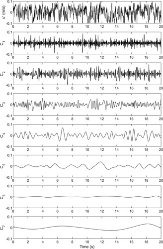
The spectra obtained with a direct Fourier transform of the signals can be highly noisy. It may be difficult to clearly distinguish the differences between the spectral plots of different cases without having very long-time data and applying several block averaging techniques etc. that occasionally over-smooth the data resulting in the loss of critical information. To obtain a smooth frequency spectrum, oscillations containing low energy levels can be extracted from the original signal. One way to perform this task is the use of the Empirical Mode Decomposition (EMD) technique of Huang et al. [25]. EMD results in intrinsic mode functions (IMF) that represent the intrinsic oscillatory modes embedded in the data. For the general properties of the IMFs and related decomposition techniques, the reader is referred to Huang et al. [25]. Thus, the original signal can be represented by the following sum of IMFs: (6) $\phi (t)=\sum _{n=1}^{N}IM{F}_n^{\phi }(t)$(6) where N is the number of IMFs. In Figure 23, the original streamwise velocity signal collected from the location $x/D^{\ast }=0.5,z/D=0.5$ for $D{45}_4$ along with the IMFs computed can be seen as an example. In this way, the turbulent velocity signal is expanded to different time scales with seven terms. The sum of the IMFs gives the original signal with high accuracy. To calculate the fluctuating energy levels, first, the Hilbert spectrum, $S_H,$ of each IMF can be computed. As is known, the Hilbert spectrum includes the variable amplitude and instantaneous frequency which highly improve the efficiency of the expansion. The resulting transform characterises the energy levels with respect to both time and frequency. The distribution of the energy according to the frequency and time can, then, be investigated. To compute the energy for a single IMF the following summation should be performed: (7) $E_n={\int }_t{\int }_f{S}_{Hn}^2(f,t)dfdt$(7)

Figure 23. Empirical mode decomposition components of the streamwise fluctuating velocity ($u^{\mathrm{\prime }}$) signal collected from the location $x/D^{\ast }=0.5,z/D=0.5$ for $D{45}_4$.

The levels can also be normalised with respect to the total energy obtained from $FP$ to facilitate the reading: (8) $E\text{\%}=\frac{E_n}{{\sum }_{n=1}^N{E}_n^{FP}}$(8) The calculation of the energy level of each IMF reveals the dominant time scales of the flow signal. The energy levels of different IMFs for different computational cases and each velocity component can be examined in Figure 24. As is seen, for the three velocity components the first four 4 IMF are dominant and contain most of the total amount of energy. Consequently, the sum of the first four IMF was selected for each computational case for the spectral analysis and the low-energy content of the remaining IMFs was neglected. In Figure 25, the first notable aspect is the significant rise in the amplitudes of the fluctuating vertical and spanwise velocities by the introduction of the dimples. Contrarily, the differences between the energy levels of the streamwise velocities may seem to be less pronounced. This is since the three-dimensional structure of the dimples mainly induces transverse and vertical flow components. By focusing on the energy levels of the different IMFs separately, it can be seen that $FP$ displays a significant rise in IMF 3. This may be due to the flow phenomenon similar to vortex shedding captured in the instantaneous shots presented in Figure 19. Since the introduction of the dimples breaks this flow structure, the amplitude of IMF 3 is damped for the dimpled cases. The information gained particularly from the investigation of the Q criterion contours suggests that the energy levels of the first 3 or 4 IMFs should present an increase representing the creation of the small-scale structures. However, it can be seen that $D{60}_{3d}$ shows equal or lower amplitudes than those of $FP$ in IMFs 1 to 3 for the streamwise fluctuations. This is partly in agreement with our previous finding that the small-scale structures that emerged in $D{60}_{3d}$ are mostly streamwise oriented which induce velocities mainly in $y$ and $z$ directions. Considering the spanwise and vertical components of the fluctuations in Figure 25, it may be seen that the order of the rise in the amplitudes associated with different computational cases is in line with the amount of the small-scale structures observed previously at different cases and the frictional performance of the surfaces. One remarkable feature of the graphic is that the energies of the high-frequency fluctuations of the vertical velocities are found to be significantly higher than those of the spanwise velocities. For instance, concerning IMF 1, the increment ratio in the amplitude of the vertical fluctuations is about 34 with respect to that of $FP$ for $D{45}_4$, while the energy of the spanwise fluctuations shows a $4.4$ times rise. This implies the relative strength of the vertical fluctuations. This is since both streamwise and spanwise structures include vertical flow components that significantly amplify the energy levels of the vertical fluctuations.

Figure 24. Energy levels of different IMFs for $u^{\mathrm{\prime }}$ (top left), $v^{\mathrm{\prime }}$ (top right) and $w^{\mathrm{\prime }}$ (bottom) ($y^{+}FP=17,D{45}_4=25,D{60}_3=28,D{60}_{3d}=28y^{+}FP=17,D{45}_4=25,D{60}_3=28,D{60}_{3d}=28$).

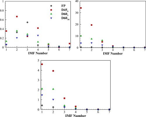
Figure 25. The original and reconstructed streamwise fluctuating velocity ($u^{\mathrm{\prime }}$) signals for different computational cases. A closer look at the reconstructed and original signals is given in the third column, black: original, red: reconstructed fluctuating velocity signal.

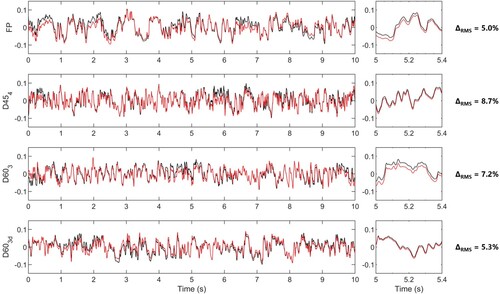
Hence a new velocity signal was generated by calculating the sum of the first four IMFs for all signals that were selected for spectral investigation. For instance, the regenerated streamwise velocity signals for different cases at $x/D^{\ast }=0.5,z/D=0.5$ are comparatively presented in Figure 25. This is also a rational approach as the spectral content of an IMF significantly reduces as the number of the IMF rises and the investigation of the very low-frequency part of the data by using a signal with a length of 20 s may result in an inaccurate representation of the spectrum. One can also define the marginal spectrum which contains the whole amount of energy of the signal and can be computed by an integration of the Hilbert spectrum over time as follows: (9) $S_h(f)={\int }_0^T{S}_H(f,t)dt$(9) The Hilbert-Huang marginal spectrum of the regenerated signals of each fluctuating velocity component, which were computed according to the procedure explained above, for the location $x/D=0$ can be seen in Figure 26. It should be noted here that the existence of energy at a frequency implies the likelihood for such a wave to have appeared locally. This is different from Fourier representation where the energy level at a frequency indicates the persistence of sine or cosine waves through a time span of the data.

Figure 26. The marginal spectrum of the fluctuating velocity components. (from top to bottom, $u^{\mathrm{\prime }},v^{\mathrm{\prime }},w^{\mathrm{\prime }}$, respectively) ($17\le y^{+}\le 28$).

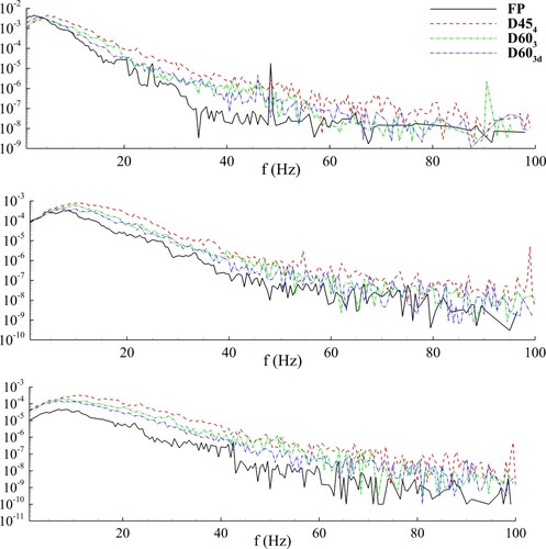
Concerning the streamwise velocity fluctuations, the existence of the dimples seems to energise nearly whole fluctuations in the range of $f>\sim 5Hz$. $FP$ displays clear peaks at around $\sim 35-55Hz$ on the centre of the dimple which appears to be shifted to higher frequencies due to the dimples. The spectra of the dimpled cases present an almost smooth structure up to $\sim 35Hz$. However, the amplitudes are still higher than that of $FP$. The plots also indicate that the energies at very low frequencies decrease to some degree. This indicates a transfer of energy from the large, coherent structures to the smaller ones. This conflicts with the finding of e.g. Tay et al. [7] who mentioned that the energy was retained at the larger scales and a greater streamwise coherence was obtained with the application of the dimples. Consequently, they observed a shift of the power spectra of the streamwise fluctuations to the lower frequencies. The current study demonstrates that although the dimples introduce streamwise vorticity and strong spanwise flow components they do not stabilise the flow, on the contrary, they create smaller flow scales that are more prone to viscous dissipation. According to the three velocity spectra obtained from the locations on the dimpled surface, the likelihood of higher frequency waves greatly increases particularly for the location corresponding to the centre of the dimple. From the mean wall shear stress distributions, we know that the friction significantly reduces around the entrance of the dimple and gradually rises towards the trailing edges. The streamwise velocity spectra presented do not display significant variations with respect to the signal location. This prevents comments on the effect of the instantaneous interaction of the boundary layer with the wall through the time span. However, we know that the minimum gain in skin friction was obtained in $D{45}_4$, which shows the highest spectral variations compared to $FP$ for the three locations considered. $D{60}_{3d}$, on the other hand, displays relatively smaller variations in the spectrum whilst presenting a larger gain in frictional drag. As mentioned previously, this suggests a negative effect of the smaller-scale structures and fluctuations on the frictional characteristics of the dimpled surfaces while the fundamental advantage comes from the vertical movement of the flow.

The spectra of the two other fluctuating velocity components ($v^{\mathrm{\prime }},w^{\mathrm{\prime }}$) demonstrate that the amplitude of almost the whole frequency range rises on the dimples’ surfaces. This implies that the application of the dimples amplifies both the large – and small-scale turbulent fluctuations in spanwise and vertical directions. This can also be seen in Figure 24 where the top right and bottom plots clearly show that the energy levels of the first four IMFs significantly rise due to the existence of the dimples with respect to $FP$. The maximum increment occurs in $D{45}_4$.

6. Concluding remarks

In this study, large-eddy simulations of the turbulent channel flow with various dimpled surfaces were presented. The drag characteristics along with the time-averaged and instantaneous flow fields were extensively examined and the effect of the dimples was investigated. The study also included a spectral analysis in terms of the Hilbert-Huang spectrum of the velocity fluctuations and revealed the effect of the dimples on the frequency domain. The critical findings of the investigations are briefly addressed as follows.

• All of the dimpled surfaces with the exception of the case with a staggered arrangement and the one involving the dimple geometry with a $d/D$ rate of $8\mathrm{\%}$ considerably reducing the frictional drag component. The cases involving larger dimples cases with a higher diameter-based Reynolds number displayed better performance in terms of skin friction. With the application of the dimples, a frictional drag reduction of up to approximately 5% was obtained.

• The Reynolds numbers based on the diameter, or the depth of the dimples are not the sole physical parameter affecting the skin friction. The combination of these Reynolds numbers along with the dimple geometry and arrangement is effective in friction reduction. Within the Reynolds number range investigated in this study, a higher $R{e}_D$ and a lower $R{e}_d$ were found to be desirable depending on the dimple configuration.

• $R{e}_d$ along with the dimple geometry is the primary parameter affecting the form drag component. A higher value of $R{e}_d$ substantially increased the form drag. The two shallower cases as well as the diamond-shaped dimpled case produced an encouraging outcome displaying almost no increase in overall drag, indicating that further studies with a slight optimisation in the dimple geometry will most possibly result in a considerable drag reduction.

• The main effective influence on the surface friction originated from the mean flow. The amount of gradient of the tangential velocities in the inner part of the boundary layer at the immediate vicinity of the bottom wall is particularly related to the sectional area variation rates of the bottom wall. Indeed, lower gradient values will decrease the overall amount of ${\overline{\tau }}_w$.

• The flow direction in high-speed regions close to the wall is also a relatively effective physical property on the frictional resistance. If a high-momentum flow portion can be orientated to the spanwise direction, even if high shear stress levels exist on the fluid adjacent to the wall, a part of them will be transferred to the spanwise flow component, which will help decrease the skin friction in the streamwise direction.

• For the Reynolds number examined in the study, the dimples did not reduce the high-frequency content of the flow and did not provide a more stable flow topology, contrary to what is pointed out in the open literature. The instantaneous flow topologies as well as the spectral investigations exposed a substantial increase in the high-frequency small-scale structure production, and a large rise in the fluctuation almost throughout the spectral span was recorded.

• Investigation of the time-averaged and instantaneous spanwise vorticities revealed an inverse relationship between the skin friction reduction performance and the level of the spanwise vorticity as well as the quantity of the smaller-scale structures in the vicinity of the wall. The flow was least disturbed by the diamond-shaped dimples, which resulted in the best skin friction reduction obtained.

• With the introduction of the dimples, strong counter-rotating pairs of alternating streamwise vortex zones were generated. However, contrary to the information given in the associated literature, the increase in the level of streamwise vorticities did not enhance skin friction reduction.

• The results suggest that future optimisation studies should consider the sectional area variation of the dimpled surface as the primary parameter by taking also the freestream velocity into account. An asymmetrical surface geometry in the $xz$ plane may also be desirable to avoid the excessive wall shear stress increment towards the trailing edge as far as possible, which was also investigated by Ng et al. [19]. The side edges should be optimised such that a sufficient spanwise flow component that affects the middle zone of the dimple is ensured.

The authors believe the present study offers essential information to understand the physics of the boundary layer flow phenomenon on the dimpled surfaces to assist the optimisation studies for reducing skin friction by means of dimples and provides a critical contribution to the literature with extensive computational simulations. Future works will involve experimental pressure measurement and flow visualisation studies in a fully turbulent flow channel facility of the University of Strathclyde with the exact physical conditions considered in this study. The experimental studies with large dimpled plates, on the other hand, will be conducted in the cavitation tunnel (ITUKAT) of Istanbul Technical University with high flow speeds to further examine the effect of the Reynolds number on drag reduction. In this way, the highly likely effect of the boundary layer thickness, which was constant in the present study due to the fixed height of the channel considered, on the flow field will also be investigated by varying the thicknesses with the use of sandpapers at the inflow.

Acknowledgments

The authors gratefully acknowledge the valuable comments, discussions and support by Prof. Mehmet Atlar of the University of Strathclyde during the preparation of this work.

The computational simulations presented in this paper were conducted at National Centre for High-Performance Computing (UHeM) of Istanbul Technical University (ITU) and Research Computing for the West of Scotland regional supercomputer centre (ARCHIE-WeSt) at the University of Strathclyde. The post-processing of the data was performed at the Computational Ship Hydrodynamics Laboratory (ID: BC03F509614) of ITU.

The computational work was carried out during the first author’s research study visit to the University of Strathclyde, which was sponsored by TÜBİTAK. The work was also supported by the Scientific Research Projects Coordination Unit of ITU (ID: MDK-2018-41461).

Disclosure statement

No potential conflict of interest was reported by the author(s).

Correction Statement

This article has been corrected with minor changes. These changes do not impact the academic content of the article.

Additional information

Funding

The work was also supported by the Scientific Research Projects Coordination Unit of ITU (ITU-BAP), (ID: MDK-2018-41461).

References

- Tacar Z, Sasaki N, Atlar M, et al. An investigation into effects of gate rudder® system on ship performance as a novel energy-saving and manoeuvring device. Ocean Eng. 2020;218:108250. doi:10.1016/J.OCEANENG.2020.108250.
- White CM, Mungal MG. Mechanics and prediction of turbulent drag reduction with polymer additives. Annu Rev Fluid Mech. 2008;40(1):235–256. doi:10.1146/annurev.fluid.40.111406.102156.
- Choi K-S, Debisschop J-R, Clayton BR. Turbulent boundary-layer control by means of Spanwise-Wall oscillation. AIAA J. 1998;36(7):1157–1163. doi:10.2514/2.526.
- Alekseev VV, Gachechiladze IA, Kiknadze GI, et al. Tornado-like energy transfer on three-dimensional concavities of reliefs-structure of self-organizing flow, their visualisation, and surface streamlining mechanisms. Trans 2nd Russ Nat Conf Heat Transfer, Heat Transfer Intensification Radiat Complex Heat Transfer. 1998;6:33–42.
- Kovalenko GV, Terekhov VI, Khalatov AA. Flow regimes in a single dimple on the channel surface. J Appl Mech Tech Phys. 2010;51(6):839–848. doi:10.1007/s10808-010-0105-z.
- Lienhart H, Breuer M, Köksoy C. Drag reduction by dimples? – A complementary experimental/numerical investigation. Int J Heat Fluid Flow. 2008;29(3):783–791. doi:10.1016/J.IJHEATFLUIDFLOW.2008.02.001.
- Tay CMJ, Khoo BC, Chew YT. Mechanics of drag reduction by shallow dimples in channel flow. Phys Fluids. 2015;27(3):035109. doi:10.1063/1.4915069.
- Burgess NK, Ligrani PM. Effects of dimple depth on channel Nusselt numbers and friction factors. J Heat Transfer. 2005;127(8):839. doi:10.1115/1.1994880.
- Chen Y, Chew YT, Khoo BC. Enhancement of heat transfer in turbulent channel flow over dimpled surface. Int J Heat Mass Transfer. 2012;55(25–26):8100–8121. doi:10.1016/J.IJHEATMASSTRANSFER.2012.08.043.
- van Nesselrooij M, Veldhuis LLM, van Oudheusden BW, et al. Drag reduction by means of dimpled surfaces in turbulent boundary layers. Exp Fluids. 2016;57(9):142. doi:10.1007/s00348-016-2230-9.
- Vida N. Three dimensional surface structure for reduced friction resistance and improved heat exchange (Patent No. US20070193726A1); 2004.
- Tay CMJ. Flow past dimpled surfaces. National University of Singapore; 2016; http://scholarbank.nus.sg/bitstream/10635/124186/1/TayCMJ.pdf.
- Wüst C. Dellen im Dach. Der Spiegel, 170–172. http://magazin.spiegel.de/EpubDelivery/spiegel/pdf/30346859; 2004.
- Tay CM, Chew YT, Khoo BC, et al. Development of flow structures over dimples. Exp Therm Fluid Sci. 2014;52:278–287. doi:10.1016/J.EXPTHERMFLUSCI.2013.10.001.
- Ligrani PM, Harrison JL, Mahmmod GI, et al. Flow structure due to dimple depressions on a channel surface. Phys Fluids. 2001;13(11):3442–3451. doi:10.1063/1.1404139.
- Turnow J, Kornev N, Zhdanov V, et al. Flow structures and heat transfer on dimples in a staggered arrangement. Int J Heat Fluid Flow. 2012;35:168–175. doi:10.1016/J.IJHEATFLUIDFLOW.2012.01.002.
- Tay CM. Determining the Effect of Dimples on Drag in a Turbulent Channel Flow. 49th AIAA Aerospace Sciences Meeting Including the New Horizons Forum and Aerospace Exposition; 2011, January 4. doi:10.2514/6.2011-682.
- Wu J, Yeo KS. Flow past Dimpled Surfaces; Part 2: Computational Study for Turbulent Flow in Dimpled Channels. Annual Report on the NUS-Airbus Collaboration under Project R-265-000-272, 597; 2011.
- Ng JH, Jaiman RK, Lim TT, et al. Geometric effects of shallow dimples in turbulent channel flows at Reτ≈ 180: a vorticity transport perspective. Flow, Turbul Combust. 2020: 1–40. doi:10.1007/s10494-020-00112-6.
- Andrade JR, Martins RS, Mompean G, et al. Analyzing the spectral energy cascade in turbulent channel flow. Phys Fluids. 2018;30(6). doi:10.1063/1.5022653
- Hussain AKMF, Reynolds WC. Measurements in fully developed turbulent channel flow. J Fluids Eng. 1975;97(4):568. doi:10.1115/1.3448125.
- Kim J, Moin P, Moser R. Turbulence statistics in fully developed channel flow at low Reynolds number. J Fluid Mech. 1987;177:133–166. doi:10.1017/S0022112087000892.
- Laufer J. Investigation of Turbulent Flow Two-Dimensional Channel. https://ntrs.nasa.gov/search.jsp?R=19930092098; 1951.
- Moser RD, Kim J, Mansour NN. Direct numerical simulation of turbulent channel flow up to Reτ=590. Phys Fluids. 1999;11(4):943–945. doi:10.1063/1.869966.
- Huang NE, Shen Z, Long SR, et al. The empirical mode decomposition and the Hilbert spectrum for nonlinear and non-stationary time series analysis. Proc R. Soc. A. 1996;454(1971):903–995.
- Ng JH, Jaiman RK, Lim TT. A numerical study for passive turbulent drag reduction via shallow dimples. 21st Australasian Fluid Mechanics Conference. https://www.nscc.sg; 2018.
- Veldhuis LLM, Vervoorty E. Drag effect of a dented surface in a turbulent flow. Collection of Technical Papers - AIAA Applied Aerodynamics Conference; 2009. doi:10.2514/6.2009-3950.
- Marino A, Ilter YK, Song S, et al.. Design specification, commission and calibration of the University of Strathclyde's Fully Turbulent Flow Channel (FTFC) facility. Rome, Italy 6th International Conference on Advanced Model Measurements Technologies for The Maritime Industry (AMT'19), 2019.
- Wang Z, Yeo KS, Khoo BC. DNS of low Reynolds number turbulent flows in dimpled channels. J Turbul. 2006;7:1–31. doi:10.1080/14685240600595735.
- Piomelli U, Liu J. Large-eddy simulation of rotating channel flows using a localized dynamic model. Phys Fluids. 1998;7(4):839. doi:10.1063/1.868607.
- Scotti A, Piomelli U. Numerical simulation of pulsating turbulent channel flow. Phys Fluids. 2001;13:1367), doi:10.1063/1.1359766.
- Nicoud F, Ducros F. Subgrid-Scale stress modelling based on the square of the velocity gradient tensor. Flow, Turbul Combust. 1999;62(3):183–200. doi:10.1023/A:1009995426001.
- Blazek J. Computational fluid dynamics: principles and applications. Third Edition. The Boulevard, Langford Lane, Kidlington, Oxford, UK: Elsevier; 2015; ISBN: 978-0-08-099995-1.
- Versteeg HK, Malalasekera W. An introduction to computational fluid dynamics: The finite volume method. Second edition,. Edinburgh Gate, Harlow, Essex, England: Pearson Education Limited; 2007; ISBN: 9780131274983.
- Issa RI, Gosman AD, Watkins AP. The computation of compressible and incompressible recirculating flows by a non-iterative implicit scheme. J Comput Phys. 1986;62(1):66–82. doi:10.1016/0021-9991(86)90100-2.
- Darwish MS, Moukalled FH. Normalized variable and space formulation methodology for high-resolution schemes. Numer Heat Transfer. 2007;26(1):79–96. doi:10.1080/10407799408914918.
- Leonard BP. The ULTIMATE conservative difference scheme applied to unsteady one-dimensional advection. Comput Methods Appl Mech Eng. 1991;88(1):17–74. doi:10.1016/0045-7825(91)90232-U.
- Ferziger JH, Perić M. Computational methods for fluid dynamics. In: Computational methods for fluid dynamics (3rd ed.). Berlin, Heidelberg: Springer; 2002. doi:10.1007/978-3-642-56026-2.
- Piomelli U, Rouhi A, Geurts BJ. A grid-independent length scale for large-eddy simulations. J Fluid Mech. 2019;766:499–527. doi:10.1017/jfm.2015.29.
- Karniadakis G, Sherwin S. Spectral/hp element methods for computational fluid dynamics. Spectral/Hp Elem Methods Comput Fluid Dyn. 2005. doi:10.1093/ACPROF:OSO/9780198528692.001.0001.
- Kiknadze GI, Gachechiladze IA, Barnaveli TT, Jr. The Mechanisms of The Phenomenon of Tornado-Like Jets Self-Organization In The Flow Along The Dimples on The Initially Flat Surface. 2009, 1–10; 2012.
- Jeong J, Hussain F. On the identification of a vortex. J Fluid Mech. 1995;285(February 2015):69–94. doi:10.1017/S0022112095000462.
- Pope SB. Turbulent flows. The Edinburgh Building, Cambridge, United Kingdom: Cambridge University Press; 2000. doi:10.1017/CBO9780511840531.