Toward the use of LES for industrial complex geometries. Part I: automatic mesh definition

Abstract

With the constant increase of computational power for the past years, Computational Fluid Dynamics (CFD) has become an essential part of the design in complex industrial processes. In this context, among the scale resolving numerical methods, Large-Eddy Simulation (LES) has become a valuable tool for the simulation of complex unsteady flows. To generalise the industrial use of LES, two main limitations are identified. First, the generation of a proper mesh can be a difficult task, which often relies on user-experience. Secondly, the ‘time-to-solution’ associated with the LES approach can be prohibitive in an industrial context. In this work, these two challenges are addressed in two parts. In this Part I, an automatic procedure for mesh definition is proposed, whereas the Part II is devoted to numerical technique to reduce the LES ‘time-to-solution’. The main goal of these works is then to develop an accurate LES strategy at an optimised computational cost. Concerning the mesh definition, because LES is based on separation between resolved and modelled subgrid-scales, the quality of the computed solution is then directly linked to the quality of the mesh. However, the definition of an adequate mesh is still an issue when LES is used to predict the flow in an industrial complex geometry without a priori knowledge of the flow dynamics. This first part presents a user-independent approach for both the generation of an initial mesh and the convergence of the mesh in the LES framework. An automatic mesh convergence strategy is proposed to ensure LES accuracy. This strategy is built to guarantee a mesh-independent mean field kinetic energy budget. The mean field kinetic energy is indeed expected to be mesh independent since only turbulent scales should be unresolved in LES. The approach is validated on canonical cases, a turbulent round jet and a turbulent pipe flow. Finally, the PRECCINSTA swirl burner is considered as a representative case of complex geometry. First, an algorithm for the generation of an unstructured mesh from a STL file is proposed to generate a coarse initial mesh, before applying the mesh convergence procedure. The overall strategy including automatic first mesh generation and its automatic adaptation paves the way to use LES approach as a decision support tool for various applications, provided that the ‘time-to-solution’ is compatible with the applications constraint. A second paper, referred as Part II, is devoted to the reduction of this time.

Keywords:

• Large-eddy simulation
• mesh adaptation
• automatic mesh generation

Acknowledgments

The authors gratefully acknowledge support from NETHUNS project under grant ANR-21-CHIN-0001-01. This work was granted access to the HPC resources of CINES/TGCC/IDRIS under the projects 2B06880 and 2A00611 made by GENCI. Part of this work has been initiated during the Extreme CFD Workshop & Hackathon (https://ecfd.coria-cfd.fr).

Disclosure statement

No potential conflict of interest was reported by the author(s).

Appendix 1. Turbulent round jet case starting from another initial mesh

To confirm that the procedure is little dependent of the flow computed on the initial mesh, the mesh convergence procedure has been applied to another initial mesh for the turbulent round jet case (Section 3.4.1). This second mesh is composed of 9, 807, 676 elements, with a mesh refinement surrounding the jet (see Figure 20-left). The automatic mesh convergence procedure is then started by using the same value to initialise $Q{C}_{1,T}$. The evolution of main quantities during the overall procedure is shown by Figure 21. The beginning of the State 1 leads first to a decrease of the number of elements due to the coarsening of the artificially refined regions. Then, the procedure is quasi similar to the procedure shown by Figure 3 with a growth of the number of elements until a final mesh composed of 8, 387, 262 elements is obtained. Note that this number of cell counts is close to the final mesh presented in Section 3.4.1. The similarities between the final meshes and the instantaneous velocity fields can be seen by comparing the Figures 20 and 2 (right part). As expected, the statistics obtained on these two final meshes are in agreement, as shown by Figure 22. This confirms that the proposed procedure is not very dependent of the initial mesh used. For a practical use, the strategy is to start the procedure with a mesh as coarse as possible, just refined to accurately represent the geometry details during the automatic mesh generation procedure (Section 4.1). It is then expected that the automatic mesh convergence will allow to design the needed mesh in the core of the computational domain.

Appendix 2. Turbulent round jet case using LIKE criterion

The proposed methodology is a mesh convergence procedure to guarantee an accurate mesh for LES. It is based on the premise that accurate LES should, at least, lead to mesh-independent mean fields, and then, a mesh-independent MKE balance. This methodology is user-independent and it does not require any a priori knowledge of the flow dynamics (as experimental data) conversely to previously proposed strategies [27–29]. In this paper, this methodology is coupled with the two criteria proposed by Benard et al. [27] to determine how the new mesh has to be generated. However, the proposed methodology is expected to work with other mesh definition criteria. The same mesh convergence procedure is then applied using the LIKE criterion [28] for the turbulent round jet case (Section 3.4.1) to confirm that.

Figure 20. Turbulent round jet configuration starting from another initial mesh. Top: Initial (left) and final (right) meshes of the centre plane of the jet flow. Bottom: Centre plane coloured by the non-dimensional instantaneous velocity norm, $|\overrightarrow{u}|/(U_1-U_2)$, computed on the initial (left) and the final (right) meshes.

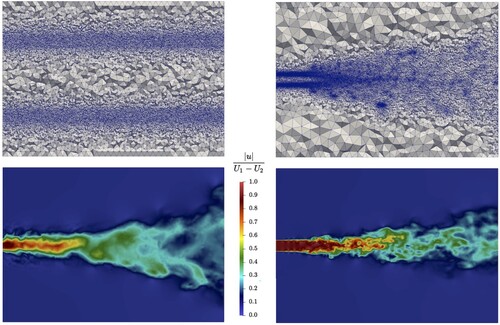
Figure 21. Evolution of the global molecular dissipation, $D_{\nu }^{\mathcal{V}}$ (top), the global transfer to TKE, $P_{\mathrm{TKE}}^{\mathcal{V}}$ (middle), and the number of elements, $N_{\mathrm{elem}}$ (bottom) during the different states of the automatic mesh convergence procedure in the turbulent round jet configuration starting from another initial mesh.

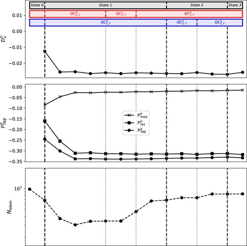
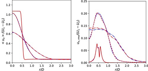
Figure 22. Comparison of round jet statistics: mean axial velocity profile (left) and rms axial velocity profile (right) at three sections: $x/D=1$ (solid line), 5 (dashed line) and 10 (dashed-dotted line). The final meshes obtained starting from the two different initial meshes are compared: case presented in Section 3.4.1 (blue) and case starting from the other initial mesh (red).

The LIKE criterion proposes to base the mesh-refinement on (9) $\mathrm{\Phi }(\overrightarrow{x})=⟨2(\nu +{\nu }_T){\overline{S}}_{ij}{\overline{S}}_{ij}⟩,$(9) which is the molecular and turbulent dissipation of the average of the overall resolved kinetic energy in LES, $K=1/2⟨{\overline{u}}_i^2⟩$. From this quantity, the adapted local mesh size, ${\mathrm{\Delta }}_a(\overrightarrow{x})$, is then defined from the initial local mesh size, ${\mathrm{\Delta }}_i(\overrightarrow{x})$, as (10) ${\mathrm{\Delta }}_a(\overrightarrow{x})=({(1-\frac{\mathrm{\Phi }(\overrightarrow{x})-{\mathrm{\Phi }}_{\min }}{{\mathrm{\Phi }}_{\max }-{\mathrm{\Phi }}_{\min }})}^{\alpha }(1-ϵ)+ϵ){\mathrm{\Delta }}_i(\overrightarrow{x}),$(10) where ${\mathrm{\Phi }}_{\min }$ and ${\mathrm{\Phi }}_{\max }$ correspond to the minimum and the maximum of Φ in the whole computational domain, and where α and ϵ are two user-parameters of the metric definition corresponding to a smoothing parameter and to the maximum refinement ratio allowed. This criterion applies this maximum refinement ratio where Φ is maximum, and keeps the initial metric where Φ is minimum. The recommended range of values to use for the criterion parameters are $0.3\le ϵ\le 0.7$ and $30\le \alpha \le 100$. In the present case, the LIKE criterion is applied with $ϵ=0.5$ and $\alpha =65$.

The proposed methodology adapted to the use of LIKE criterion is finally simpler than the methodology proposed for the two criteria (Section 3.3). Starting from the same coarse mesh composed 307, 806 elements, the mesh is adapted based on the metric definition of the LIKE criterion, Equation (10(10) ${\mathrm{\Delta }}_a(\overrightarrow{x})=({(1-\frac{\mathrm{\Phi }(\overrightarrow{x})-{\mathrm{\Phi }}_{\min }}{{\mathrm{\Phi }}_{\max }-{\mathrm{\Phi }}_{\min }})}^{\alpha }(1-ϵ)+ϵ){\mathrm{\Delta }}_i(\overrightarrow{x}),$(10) ), after each statistical time window, $T_w=170R/(U_2-U_1)$. This is repeated until the deviations of the global molecular dissipation, $\mathrm{\Delta }{D}_{\nu }^{\mathcal{V}}$, and the global turbulent production, $\mathrm{\Delta }{P}_{\mathrm{TKE}}^{\mathcal{V}}$, are both smaller than 0.05. Figure 23 shows the evolution of the global molecular dissipation and the global turbulent production as a function of the number of elements during the mesh convergence procedure. The procedure based on LIKE criterion is compared to the procedure based on $Q{C}_1$ and $Q{C}_2$ criteria presented in Section 3.4.1. At the end of the mesh convergence procedures, the global molecular dissipation and the global turbulent production are very similar, showing that the same global MKE balance is recovered. However, the procedure based on LIKE criterion leads to a final mesh composed by 102,354,009 elements, which is important in comparison with the final mesh composed by 8,125,037 elements obtained with the procedure based on $Q{C}_1$ and $Q{C}_2$ criteria. One reason is that the LIKE criterion is not able to coarsen the mesh during the adaptation steps. The mesh influence on the statistics prediction is shown in Figure 24. The mean and root mean square (rms) axial velocities obtained with the final meshes are compared with the reference case. The final meshes obtained with both procedures are in good agreement with the reference case. For the procedure based on LIKE criterion, results on the second to last mesh are also considered. This mesh is composed by 13,902,402 elements. For this mesh, first- and second-order statistics are in good agreement except for the rms axial velocity at the beginning of the jet which are significantly under-predicted. This under-prediction is corrected by the last adaptation step. This confirms that the proposed mesh convergence procedure built to guarantee a mesh-independent MKE balance is able to lead to accurate LES for various mesh adaptation criteria.

Figure 23. Evolution of the global molecular dissipation, $D_{\nu }^{\mathcal{V}}$ (top), and the global transfer to TKE, $P_{\mathrm{TKE}}^{\mathcal{V}}$ (bottom) as a function of the number of elements, $N_{\mathrm{elem}}$ during the automatic mesh convergence procedure based on LIKE criterion (red line) and based on $Q{C}_1$ and $Q{C}_2$ criteria (blue line).

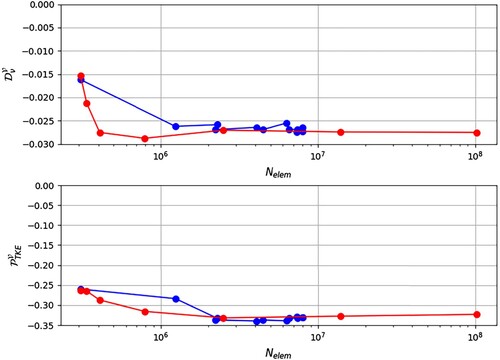
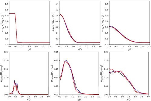
Figure 24. Comparison of turbulent round jet statistics: reference case (black), final mesh for the procedure based on $Q{C}_1$ and $Q{C}_2$ criteria (blue), final mesh for the procedure based on LIKE criterion (red, solid line) and the mesh obtained just before (red, dashed line). Mean axial velocity profile (top) and rms axial velocity profile (bottom) at three sections: $x/D=1$ (left), 5 (middle) and 10 (right).

Additional information

Funding

This work was supported by Agence Nationale de la Recherche [ANR-21-CHIN-0001-01].