The climate test: a tool to evaluate alignment of energy infrastructure decisions with climate goals

ABSTRACT

Although rapid transition away from fossil fuels will be required to limit warming to any agreed upon level, long-lived fossil energy infrastructure buildout continues largely unabated. Many nations around the world have laws requiring regulators to meaningfully assess potential climate impacts when reviewing proposals for new fossil fuel infrastructure projects such as oil and gas extraction leases, major transmission pipelines, and power plants. However, reviewing agencies often report lack of appropriate tools to objectively assess the climate impacts of individual fossil fuel infrastructure projects, and to determine the significance of these impacts. Here we present a novel methodology to fill this critical gap by providing a science-based decision support tool, a ‘climate test’, for use in determining an infrastructure project’s carbon emissions significance. The climate test defines emissions significance quantitatively according to a project’s consistency with region-specific constraints and characteristics of climate mitigation pathways, considering both emissions and energy systems characteristics over the project’s lifespan. We showcase the tool here, using an example of a natural gas pipeline to explore how often and under what conditions the project would ‘pass’ the climate test with an emissions significance result of ≤1, which indicates alignment with a 1.5°C goal. For this project, less than 1.2% of 10,000 scenarios yielded significance values ≤1, suggesting a high likelihood that the project has a significant climate impact, a determination that would be robust to uncertainty for such a project. This emission-based metric represents a first step toward a broader framework to align project-level infrastructure decisions – including and beyond new fossil energy projects – with climate, as well as economic and societal, policy goals.

Key policy insights

• This novel ‘climate test’ tool is suitable to support U.S. regulators in meeting their statutory requirements to assess the significance of climate impacts for fossil energy infrastructure projects on an individualized basis.

• While the tool was designed based on specific gaps identified in the U.S. system, it can readily be adapted for use in other non-U.S. regulatory contexts.

• Widespread implementation of such a climate test tool would help the US, and other nations that use it, to act consistently with their national and international climate commitments by aligning individual project-level decisions with pathways to limiting warming.

• By defining project significance in the context of both the emissions constraints and energy needs of a warming-limited world, this climate test tool provides decisionmakers with integrated and nuanced analytical information necessary to responsibly manage both energy and climate policy objectives.

KEYWORDS:

• Fossil fuels
• decision analysis
• energy policy
• climate policy frameworks
• environmental impacts
• policy instruments

1. Introduction

To avert the worst effects of climate change, future carbon dioxide (CO₂) emissions need to be kept within a tight and finite carbon budget, with annual emissions falling to net-zero by midcentury and net-negative after (IPCC, 2021b; 2018). Realistically, this can only be accomplished through large and rapid declines in the use, and accompanying development, of fossil energy infrastructure (Rogelj et al., 2018; IEA, 2021). However, national regulators around the world continue to approve new long-lived fossil fuel projects, ranging from wells to pipelines and power plants, at a level that is collectively inconsistent with national and international climate goals to limit warming (Achakulwisut et al., 2021).

Beginning with the National Environmental Policy Act (NEPA) in the U.S., the practice of formal environmental impact assessment (EIA) has spread to become common around the world, intended to guide regulatory decisions on projects with the potential to create significant environmental harm (Abaza et al., 2004). Climate change has naturally become a large component of this practice, with researchers (Doelle, 2018), professional societies (Byer et al., 2018), and governments (U.S. Council on Environmental Quality, 2016) publishing guidelines. However, in the U.S., despite laws and court rulings mandating that EIAs quantify individual project-level greenhouse gas emission (GHG) impacts and assess their climate significance, current project-level assessments regarding the climate significance question are generally inconclusive at best. New fossil fuel projects are virtually never rejected for reasons related to climate (Sierra Club v. FERC, 2017).

We determined, based on our review of project assessments and court decisions challenging them, that agencies lack a reliable metric for assessing the climate significance of GHG emissions. The GHG assessments either used U.S. agencies’ so-called ‘proxy methodology’, i.e. the comparison of project emissions to national or global emissions, whose inadequacy we explain below, and more recently the Social Cost of Carbon (SCC), whose insufficiency as a measure of significance we also explain (350 Montana v. Haaland, 2022; Montana Envt’l Info. Ctr. v. Haaland, 2022; Utah Physicians for a Healthy Environment v. BLM, 2021; Montana Envt’l Info. Ctr. v. Office of Surface Mining, 2017; Wildearth Guardians v. Zinke, 2019; High Country Conservation Advocates v. Forest Service, 2014). Some courts and agencies have referenced the lack of a significance assessment methodology, usually focusing unnecessarily narrowly on the specific problem of how to tie project emissions to specific climate impacts on natural systems (Sierra Club v. FERC, 2017; Wilderness Workshop v. BLM, 2018; Western Org. of Res. Councils v. BLM, 2018; San Juan Citizens Alliance v. BLM, 2018). The U.S. Federal Energy Regulatory Commission (FERC) expressly recognized the lack of a viable climate significance methodology in its recently updated draft GHG policy statement. They note, ‘To date, no federal agency, including the Commission, has established a threshold for determining what level of project-induced GHG emissions is significant’ (FERC, 2022).

The present work describes a science-based decision support tool – the ‘climate test’ – we developed to address the disconnect between the statutory mandate to assess individual projects’ climate significance and the currently inadequate processes by which that mandate has been implemented. The resulting tool is suitable and ready for use in the U.S. context, where the authors are based. However, the climate test framework can be readily adapted to any nation where data are available to assist informed decision-making.

2. Background

We reviewed current GHG impact assessment processes for new fossil fuel infrastructure projects with a focus on the U.S. and identified three fundamental flaws common to these processes. These include: (1) incomplete assessment, (2) inappropriate context for analysis, and (3) lack of decision criteria.

First, EIA reviews across agencies are inconsistent and have often contained incomplete GHG emissions accounting. Project-level analyses, particularly of midstream projects like pipelines, will often fail to consider full life-cycle emissions of the project, assessing only direct emissions (i.e. Scope 1 emissions in the GHG Protocol (WRI and WBCSD, 2004)), or sometimes including downstream but not upstream indirect emissions (i.e. GHG Protocol Scope 3) (Burger & Wentz, 2017). However, all fossil fuel projects are part of an interconnected energy supply chain spanning from fuel production and processing to transport, distribution, and ultimately in the vast majority of cases, combustion for energy or heat (EIA, 2019). The pipeline’s direct emissions may be small, but those it enables upstream and downstream in the supply chain are not. Failure to consider and quantitively assess this systemic interconnection underestimates the functional role of the project and skews conclusions about the significance of its climate impacts.

Second, agency reviews use contexts for analyzing project emissions that are inappropriate in multiple ways. For one thing, the proxy methodology in these reviews compare global or national emissions at a single snapshot in time, which is inappropriate because the projects are long-lived investments that will function and pollute for decades to come. As such, each new project will become part of a complex and constantly evolving energy system that is already filled with operating fossil infrastructure, which will continue to consume the remaining climate budget over time. Additionally, simply taking a snapshot of project versus global emissions and assuming that comparison is representative for the future time period it will operate ignores a fundamental feature of climate change: it is a cumulative process. That means holding total emission levels steady over time is not neutral to climate impact, it is an impact in itself. Continued emissions at status quo levels would passively but certainly result in a constant rate of warming, not a constant temperature. Only a world where emissions decline to net-zero, and remain net-negative for some period after, can ever produce a stable climate system, where warming is halted. Anything else neglects the very basics of climate science and downplays the need – and the stated intent of domestic and international policy commitments – to reduce future emissions.

Third, decision-makers lack objective criteria for determining whether the emissions of a project will have a significant climate impact. Their often-used proxy methodology comparing project emissions to sectoral, national, or global emissions, or even to the remaining carbon budget, yields a result that is both misleading and fundamentally uninterpretable in terms of climate significance. This type of comparison trivializes the project’s climate impact, since even the largest project’s emissions would be dwarfed by comparison to total national or worldwide emissions. More importantly, as acknowledged by the FERC’s draft GHG policy statement, this type of evaluation metric alone provides no objective basis to determine at what level those new emissions become significant.

Some U.S. agencies have recently attempted to address one or more of these analytical deficiencies, but the scope of their analysis is limited. In June 2022, following a court loss, the Bureau of Land Management (BLM) published a draft supplemental assessment of the Willow Master Development Project, a large oil drilling project in Alaska’s North Slope (BLM, 2022). Along with including total direct and indirect GHG emissions over the project’s lifetime, BLM included comparisons of project emissions to climate goals such as the 2030 target of 50–52% net-GHG reduction beyond the standard, current annual regional emissions (BLM, 2022). However, this additional reporting and analysis still falls short of what is needed, because BLM failed to offer any rational means for understanding the significance of these comparisons. As a result, BLM drew no conclusion or determining whether the project’s emissions are significant with respect to climate, stating only that ‘all projects may cumulatively have a significant impact on global climate change’ (BLM, 2022).

Additionally, the U.S. office overseeing cross-agency NEPA implementation, the Council on Environmental Quality (CEQ), released an interim draft guidance policy in January 2023 that raises many of the recommendations underlying our climate test – including the need to consider both direct and indirect emissions over time, and to ‘place emissions in relevant context, including how they relate to climate action commitments and goals’ (CEQ, 2023). However, these guidelines provide no methodology by which to implement those recommendations.

Finally, the SCC is increasingly being deployed in U.S. agency impact assessments (FERC, 2022), including in the Willow analysis (BLM, 2022), and is recommended by the recent CEQ draft guidance (CEQ, 2023). Agencies use SCC to convert GHG emissions to a dollar figure representative of climate-related damages expected to be caused around the world from their marginal warming effect (Smith & Braathen, 2015). While monetization is useful to enable agencies and the public to consider effects of a project’s GHG emissions in familiar economic terms, it does not provide an actionable criterion for determining whether any given level of monetized damage is significant or not on its own. Similarly, using SCC as part of a traditional cost–benefit framework (Hein et al., 2019) also lacks tethering to the fundamental question of whether the subject emissions are significant to driving climate impacts.

Outside of the U.S., other nations appear to be grappling with the same questions in their approaches for evaluating climate impact significance (Mayembe et al., 2023; van der Bank & Karsten, 2020; EarthLife Africa Johannesburg v Minister of Environmental Affairs and Others, 2017). In the U.K, their new Climate Compatibility Checkpoint, for example, was designed to look at alignment of oil and gas operations with net-zero by 2050 climate goals but focuses on comparing reductions in direct, operating emissions from the sector as a whole rather than informing individual project decisions (BEIS, 2022). Similarly, Canada is in the process of developing guidance for ‘best-in-class’ GHG emissions performance for oil and gas projects, but it does not prescribe an analysis method, nor does it appear to consider downstream Scope 3 combustion emissions (ECCC, 2022). In South Africa, following the Earthlife Africa case (van der Bank & Karsten, 2020; EarthLife Africa Johannesburg v Minister of Environmental Affairs and Others, 2017), where the High Court ultimately revoked the Thabametsi coal plant’s emission authorization due to insufficient climate impact assessment at the ministries, the national Ministry of Forestry, Fisheries, and Environment has recently issued draft guidance in 2021 (DFFE, 2021) laying out principles to address many of the aforementioned issues of emissions scope (including direct and indirect) and contextualizing with climate goals (i.e. Paris NDC emission trajectories), but appears not to have finalized.

3. Methodology: climate test tool development

3.1. Conceptual framework and design of the climate test

Our goal in designing the climate test is to provide government agencies – as well as project proponents, stakeholders, and the public – with a consistent, scalable, and evidence-based method for assessing the climate significance of GHG emissions that avoids the three deficiencies in current agency methods we have described. This method needs to be applicable to any type of fossil fuel energy infrastructure, and to be equipped with objective, easily interpretable decision criteria for use within current legal structures. No such method currently exists in the literature, and hence our tool makes a novel contribution to fill that gap.

Non-governmental organizations have discussed the need for a climate test during the past decade, but the term has mainly described a concept and set of principles (“ClimateTest.Org” 2016; Noble & Brady, (2017). None have put forward an analytical framework of the scope or nature we propose here. Among the select white papers published in the grey literature concerning climate testing, the focus was on mainly identifying the types of parameters that should be included and whether it should be based on emissions or economic factors (Noble & Brady, 2017; Hasselman & Erickson, 2022; Erickson & Lazarus, 2018). In the academic literature, Jaccard et al. proposed a methodology they referred to as a ‘climate test model’, but it focused on economics rather than emissions (Jaccard et al., 2018). While these references provided us useful background and ideas, they either lacked quantitative detail or offered too limited connection to current regulatory processes to be useful as a decision support tool.

We designed the climate test metric to address the three flaws we identified in current GHG assessment methods by: (1) fully assessing the project’s impact drivers (i.e. lifetime, lifecycle emissions); (2) analyzing the project’s impacts in the most appropriate context for the phenomenon, i.e. cumulatively over time, as well as in the context of the existing energy system and relative to climate goals; and (3) evaluating the project’s GHG impact significance on an objective and integrated basis – i.e. its function, which is the energy it provides to the system.

To address the problem of incomplete and inconsistent emissions accounting, our climate test tool specifies that project emissions be quantified using lifecycle assessment scoped to include both indirect (Scope 3) and direct (Scope 1), GHG emissions thus capturing the full supply chain. To address agencies’ failure to assess emissions in proper context, we specified that the project’s emissions and energy contribution be quantified over its operational timeframe, in relation to other existing sources of emissions, in the context of dynamic conditions for reaching a specified climate goal, such as limiting warming to 1.5℃. Finally, to address the lack of an objective basis for determining climate significance of a project’s emissions, we structured the final decision metric to be based on a comparison between the emissions impact (i.e. carbon budget to be consumed by a project) and its relative function (i.e. energy contributed to a warming-limited system). This comparison yields a simple numeric result that communicates a projects’ emissions significance in terms of its degree of alignment with characteristics of a warming-limited world.

Like any good policy decision tool, the climate test stipulates use of reliable, transparent, and credible data for assessing individual projects. Data specific to the fossil fuel project under review should be provided by proponents where available (e.g. via project documentation). Where unavailable, we provide default value from literature. As an additional strength, the test’s parameterized nature allows for robust decision-making under uncertainty (Marchau et al., 2019). The values of any of the input variables, including the specified climate goal or project characteristics, can be varied, enabling supplemental exploration and statistical analyses to test alternative assumptions, evaluate influence of specific inputs, strengthen the conclusion regarding significance, and guard against biased estimates. Finally, the climate test’s defining feature is that it is quantitative and mathematically structured to yield an objective and simple ratio result from which emissions significance can be interpreted: ≤1 for projects that are consistent with the climate goal and >1 for projects that are not.

3.2. The climate test emissions significance metric

The climate test, illustrated in Figure 1, assesses a project’s emissions impact over its lifetime to determine whether, and to what degree, that project’s emissions intensity is consistent with the constraints and characteristics of a world where the specified climate goal can be met.

Figure 1. Conceptual framework, data source types, and component inputs metrics for the climate test decision metric to evaluate emissions significance of individual fossil fuel projects.

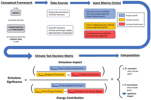
Computationally, the climate test boils down to a compound metric, called emissions significance, that weighs a project’s emissions impact in the climate goal scenario against its energy contribution in that same scenario, as shown in equation (1). (1) $\mathrm{Emissions}\mathrm{Signficance}={\displaystyle \frac{\mathrm{Emissions}\mathrm{Impac}{t}_{\mathrm{region},\mathrm{goal}}^{\mathrm{gas}}}{\mathrm{Energy}\mathrm{Contributio}{n}_{\mathrm{region},\mathrm{goal}}}}$(1) The emissions impact numerator is a proxy indicator for warming. It is calculated as the percentage of climate goal-specified regional carbon budget¹ that would be cumulatively consumed by the project’s lifecycle emissions over the course of its lifespan, from the start of construction through the end of operation. Additionally, it accounts for committed emissions from other extant fossil fuel infrastructure projected to be operating during that period (equation (2)) to show the real cost of adding anything new into a dwindling carbon budget. (2) $={\displaystyle \frac{{\sum }_{t=t_0}^{t_0+\mathrm{\Delta }{t}_c+L}\mathrm{Lifecycle}\mathrm{Emission}{s}_{\mathrm{project}}^{C{O}_2}\left(t\right)}{\left\{\mathrm{MAX}:0,{\sum }_{t=t_0}^{t_0+\mathrm{\Delta }{t}_c+L}\left(\mathrm{Budgeted}\mathrm{Emission}{s}_{\mathrm{US},1.5C}^{\mathrm{Energy}C{O}_2}\left(t\right)-\mathrm{Committed}\mathrm{Emission}{s}_{\mathrm{US}}^{\mathrm{Energy}C{O}_2}\left(t\right)\right)\right\}}}$(2) where: t = model annual time period

• t₀=  model start year = project construction start year

• Δt_c= project construction duration (years)

• L =  project operating lifespan (years)

The energy contribution denominator provides the test’s objective basis for determining significance by grounding evaluation of a project’s emissions impact in its function of providing energy. It is calculated analogously to emissions impact, as the project’s percent contribution to future fossil energy demand in a 1.5°C world, not already met by existing fossil energy infrastructure over that same period (equation (3)). $\mathrm{Energy}\mathrm{Contribution}={\displaystyle \frac{\mathrm{Total}\mathrm{Energy}\mathrm{Supplied}\mathrm{by}\mathrm{Project}}{\mathrm{Total}\mathrm{Unmet}\mathrm{Fossil}\mathrm{Energy}\mathrm{Demand}\mathrm{under}\mathrm{Climate}\mathrm{Goal}}}$ (3) $={\displaystyle \frac{{\sum }_{t=\mathrm{start}}^{t_0+\mathrm{\Delta }{t}_c+L}\mathrm{Energy}\mathrm{Supplie}{d}_{\mathrm{project}}\left(t\right)}{\left\{\mathrm{MAX}:0,{\sum }_{t=t_0}^{t_0+\mathrm{\Delta }{t}_c+L}\left(\mathrm{Fossil}\mathrm{Energy}\mathrm{Demande}{d}_{U.S.,1.5C}\left(t\right)-\mathrm{Existing}\mathrm{Fossil}\mathrm{Energy}\mathrm{Supplie}{d}_{U.S}\left(t\right)\right)\right\}}}$(3) Because both numerator and denominator are scoped to the same geographic, temporal, and climate scenario context and share a computational structure, the climate test would produce a result of 1 if the project’s emissions intensity perfectly matches the necessary energy system transition in a warming-limited scenario. Since a result of >1 indicates the project is not aligned with the constraints and characteristics of meeting the specified climate goal, it can be interpreted to indicate significant individual impact with respect to climate change. The more inconsistent a project is with the specified climate future, the higher the emissions significance number will be enabling intuitive comparison between alternatives. Conversely, an emissions significance result ≤1 suggests the project’s emissions intensity (per unit of energy) is aligned with the climate goal scenario, and not likely to yield relatively significant climate impact.

The fossil fuel demand factored into the denominator is based upon scenarios of demand in a world on track to meet the climate goal of limiting global warming to 1.5°C with low- or no-overshoot, as modelled for the Intergovernmental Panel on Climate Change (IPCC)’s Special Report on 1.5°C of warming (IPCC, 2018, p. 5; Huppmann et al., 2018). Results of a second analysis using a related climate goal, net-zero CO₂ emissions by 2050, as modelled for Princeton University’s U.S.-specific Net Zero America (NZA) study, are also presented in Appendix B for corroboration (see Supplementary Material). The scope of the denominator is limited to fossil energy need, as a key purpose of the test is to provide insight on the question of whether a particular project is consistent with the sharp decline specifically in fossil fuel use projected to occur on a path to net zero emissions. This approach makes the test particularly useful in responding to the frequent statement by project proponents that fossil fuels cannot be discontinued immediately and need to be part of our energy system in coming decades. The climate test provides a quantitative assessment of that loosely framed construct, which as explained below, demonstrates that most (if not all) individual fossil fuel projects are inconsistent with climate goals. A more detailed description of the metric’s analytical components can be found in Appendix A-1 (Supplementary Material). The Supplementary Data file SD1 also includes an active beta version of the climate test tool in spreadsheet form, with live formulas for transparency and validation.

3.3. Case study data and analysis

We selected a real-world project, the Pacific Connector natural gas transmission pipeline (FERC, 2019) to serve as an example case study and primary data source for applying the climate test. Gas pipelines are good illustrative examples because gas, as the least carbon-intensive fossil fuel, represents an edge case that should have the highest likelihood among its resource class of yielding results close to the test’s structural decision point of 1. Additionally, midstream projects like pipelines illustrate the importance of including full lifecycle emissions, so as to evaluate the climate impacts of a project in the context of its function and the integrated supply chain.

To simplify the analysis for U.S. scope, we chose to assert that all gas transmitted by the pipeline project (up to capacity of 1.2 billion cubic feet, or 0.034 billion cubic metres, per day) would feed domestic combined cycle natural gas power plants rather than a liquified natural gas export facility (FERC, 2019). We additionally assumed pipeline construction began in 2020 and continued for 5 years (FERC, 2019).

We conducted four analyses to explore the performance of the climate test tool. First, we calculated a single baseline result using the best single point estimates of each project-related and existing infrastructure-related variable. Then, because uncertainty is an unavoidable challenge of any prospective analysis, we conducted two 10,000-simulation Monte Carlo analyses to explore the statistical likelihood of getting a ‘passing’ emissions significance result of ≤1 in conditions other than the baseline. For the first Monte Carlo analysis, we tested the full range and likelihood of climate test results under the widest possible exploratory range of potential conditions, including likely unrealistic conditions such as extremely short project lifespans or the immediate shutdown of large portions of committed emissions. The second Monte Carlo analysis looked at a narrower, more ‘reasonable’ range of input values that were judged to be more reflective of realistic conditions and draw more realistic conclusions. These analyses also enabled us to assess what combinations of randomly generated variables, if any, would yield a climate-goal consistent conclusion to further guide decisionmakers. Finally, we conducted single factor sensitivity analyses to examine the effects of each of the different variables on the results of the emissions significance metric and of its component parts (i.e. the numerator and denominator in equation (1)), holding all other variables equal at their respective baseline values.

Baseline, or best initial estimate, values for each of the input variables for the climate test metric came from a variety of sources (Table 1).

Table 1. Summary of data inputs (baseline and Monte Carlo analysis ranges) used for the climate test case study of a natural gas pipeline.

Cat.	ID	Fig 2 ID	Climate significance metric parameters:	Type	Input influencing value	Distribution Type	Simulation value ranges
			Key inputs, intermediate result values				Units	Baseline	Exploratory range (n = 10,000)			Reasonable range (n = 10,000)
									Min	Median	Max	Min	Median	Max
Climate Scenario Characteristics (CS)	CS-1	(vi)	Climate scenario ID	Input	Source: IPCC 1.5°C Report Database (IAMC/IIASA) (Huppmann et al., 2018)	Discrete – uniform	–	N/A – Median across scenarios	Compatible model scenarios Labelled: 1–18			Compatible model scenarios labelled: 1–18
	CS-1A	(5)	Budgeted carbon emissions*	Intermed. result	CS-1, P-1Aiia-d	Indirect	GtCO2	66.90	20.61	62.14	103.71	30.63	64.36	98.20
	CS-1B	(8)	Fossil energy demand				EJ	1393.92	354.31	1347.42	3464.43	734.44	1363.61	2853.11
Project Characteristics (P)	P-1	(A)	Project lifecycle emissions	Intermed. result	P-1A, EES-1	Indirect	GtCO2	0.668	0.000156	0.423	1.297	0.107	0.502	1.076
	P-1A	=(2) + (3)	Project direct emissions	Intermed. result	Source: Project documentation (FERC, 2019); P-1Aiia-d, P-1Aiii	Indirect	GtCO2	0.00797	0.000087	0.0051	0.0152	0.0013	0.0060	0.0126
	P-1Aiia	(i)	Project construction start year	Input	Source: Project documentation (FERC, 2019) or default	None	–	2020	2020			2020
	P-1Aiib	(ii)	Project construction duration	Input		None	Years	5	5			5
	P-1Aiid	(iii)	Project operating lifespan	Input		Triangle	Years	26	0.3	25.5	49.7	10.2	25.5	39.9
	P-1Aiii	(iv)	Project capacity utilization factor	Input		Triangle	%	95.8%	1%	69%	100%	26%	77%	100%
	P-1B	(1)	Project indirect emissions: upstream	Intermed. result	P-1Ai, P-1Aiia-d, EES-1A	Indirect	GtCO2	0.085	0	0.053	0.223	0.010	0.063	0.181
	P-1C	(4)	Project indirect emissions: downstream	Intermed. result	P-1Ai, P-1Aiia-d, EES-1B	Indirect	GtCO2	0.576	0	0.365	1.117	0.09243	0.432	0.927
	P-2	(C)	Project lifetime energy supplied	Intermed. result	P-1Ai, P-1Aiia-d	Indirect	EJ	11.90	0.1295	7.561	22.67	2.003	8.962	18.90
Existing Energy System Characteristics (EES)	EES-1	(v)	Indirect emissions factor ID	Input	Source: NETL LCA (Littlefield et al., 2019)	Discrete – non-uniform	–	2 (mean)	1 (2.5%ile)	2 (mean)	3 (97.5%ile)	1 (2.5%ile)	2 (mean)	3 (97.5%ile)
	EES-2	(6)	Committed emissions	Intermed. result	Source: Tong et al. (2019), P-1Aii, EES-2A,EES-2B,EES-2C	Indirect	GtCO2	50.35	10.93	41.94	55.87	36.06	49.67	56.21
	EES-2A	(x)	Additive factor for upstream activities	Input	Source: NETL LCA (Littlefield et al., 2019)	Triangle	%	10%	5.54%	13%	20.40%	5.63%	13%	20.4%
	EES-2B	(vii)	Share of committed emissions realized by target date	Input	N/A	Triangle	%	100%	0.40%	70.70%	100%	80.1%	94.1%	100%
	EES-2C	(viii)	Years to target date for linear decline to share of committed emissions realized	Input	N/A	Triangle	years	0	0.04	17.68	25.00	10.07	20.61	25.00
	EES-3	(9)	Committed energy: via emission intensity	Intermed. result	EES-2, EES-3A	Indirect	EJ	725.15	151.93	589.58	788.85	507.61	698.42	752.58
	EES-3A	(ix)	Linear percentage change in committed emissions intensity to 2050	Input	N/A	Triangle	%	0%	−20%	0%	20%	−5%	0%	5%

For climate scenario inputs (green rows with CS prefix in Table 1), such as budgeted CO₂ emissions and fossil energy demand for the 1.5°C goal over the timeframe analyzed in our case study, baseline values came from the IAMC 1.5C Scenario Explorer database (Huppmann et al., 2018). We screened this larger dataset for regionally appropriate data and identified 18 climate model scenarios; and calculated the median of their time series data on CO₂ emissions from energy use and energy consumption from coal, oil, and gas. A more detailed description of the complete screening process and resulting selections can be found in Appendix A-1, and Supplementary Data file SD1.

For project-specific inputs (blue rows with P prefix in Table 1), such as pipeline capacity, average utilization factor, and direct emissions from construction and operation, baseline values came from the project’s documentation provided for the review process (FERC, 2019) Although pipelines can have operational lifespans well beyond 50 years (INGAA, 2019), we opted to model baseline project operations only through to the end of 2050, which corresponds to timing for reaching net-zero emissions articulated in many climate goal scenarios. Absent project details to the contrary, we assumed constant throughput in all years. Baseline values for indirect GHG emissions upstream extraction and processing life cycle stages as well as from downstream distribution were calculated using national average emission factors from the National Energy Technology Laboratory (NETL) lifecycle analysis database (Littlefield et al., 2019). Baseline values of downstream combustion emissions were more simply calculated using the stationary combustion emission factor for gas from EPA (EPA, 2016). As a default, we treat all emissions as additive, but other realities can be explored with sufficient justification.

For existing energy system inputs (yellow rows with EES prefix in Table 1), baseline values for committed emissions were based upon Tong and colleagues’ data published in the literature (Tong et al., 2019). However, because this source mentions having excluded upstream and midstream emissions, we include an additional variable correction factor, set at 10% in baseline,² to augment their partial estimate and expand the scope to better match the full lifecycle perspective of the other metric elements. In absence of better data, we approximated baseline existing energy supply projections from committed emissions data by estimating a baseline emissions intensity for existing energy system using coal, oil, and gas energy production data from the U.S. Energy Information Administration (EIA, 2019). In the baseline, we assumed emissions intensity of the existing fossil energy supply remains constant at 2018 levels over the analysis period. However, because it is possible that the emissions intensity of the extant fleet will change as the system evolves, we embedded variables that enable modification to the committed emissions and existing energy supply trajectories. More detail on the committed emissions and existing energy supply calculations is set forth in Appendix A-1 (Supplementary Material).

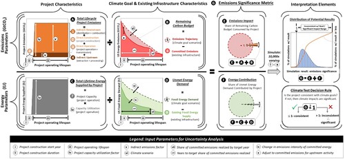
For each of the two Monte Carlo analyses, we developed ranges and distributions for variable inputs about the project, the climate goal, and the existing energy system, as summarized in Table 1 alongside baseline values for comparison. Figure 2 illustrates how each variable combines and relates to one another to produce a distribution of climate test metric results in this analysis.

Figure 2. Graphical schematic of climate test components, labelled (A)–(G), and relationship to input parameters, labelled (i)–(x), that were varied during Monte Carlo and single factor sensitivity analyses. The graphs in the top row are all emissions-related, with units of GtCO₂, and combine to create the emissions impact component (E), or the numerator of the emissions significance metric (G). Similarly, the graphs in the second row are all energy-related, with units of EJ, and combine to create the energy contribution component (F), or the denominator of the emissions significance metric (G). Across rows, from left to right, the graphs in the leftmost column are all characteristics of the project being evaluated, which are then used to compare the project to the characteristics of the climate goal, given existing energy system characteristics, found in the middle column. Together, simulated variations in the input parameter values drive variation in the emissions impact and energy contribution component results, and produce a distribution of emissions significance metric results, as shown in the far right graph. Each simulation result is judged against the same decision criteria of ≤1 for projects consistent with the climate goal and >1 for projects with a significant climate impact.

4. Results and discussion

4.1. Baseline results

Initial, baseline climate test evaluation showed that the example gas pipeline project is not consistent with meeting the 1.5℃ climate goal we specified.

Over the lifetime of the project, or the period when the project was expected to emit, from 2020 to 2025 for construction and 2025 to 2050 for operation, the pipeline is expected to emit a total of 0.667 billion tonnes of CO₂ (GtCO₂) from direct and indirect Scope 1–3 activities. This amount is equivalent to 1% of the total budgeted U.S. energy sector CO₂ emissions over those years (66.9 GtCO₂), according to the median estimate from the 18 selected IPCC 1.5℃ scenario pathways we used. However, already existing fossil energy infrastructure also projected to operate over that same period would emit a total of 50.4 GtCO₂ in Scope 1–3 emissions, leaving just 16.5 GtCO₂ in remaining carbon budget for new project emissions. Therefore, the emissions of the pipeline project would be more accurately understood to consume just over 4% of the remaining carbon budget consistent with meeting the 1.5℃ climate goal (equation (4)). (4) $\mathrm{Emissions}\mathrm{Impact}={\displaystyle \frac{0.667\mathrm{GtC}{O}_2\mathrm{Total}\mathrm{Lifecycle}\mathrm{Project}\mathrm{Emissions}}{\left(66.9\mathrm{GtC}{O}_2\mathrm{Climate}\mathrm{Goal}\mathrm{Budgeted}\mathrm{Emissions}\right)-(50.4\mathrm{GtC}{O}_2\mathrm{Committed}\mathrm{Emissions}})=4.04\text{\%}}$(4)

Most of the project’s lifecycle emissions (∼86%) come from combustion of the gas it delivers to the power sector. Over the 25-year operational lifespan that we tested, the pipeline is assumed to provide a total of 11.9 Exajoules (EJ) of primary energy to meet demand. During that same period for the 1.5℃ climate scenario, a total demand of 1393 EJ of primary fossil energy is expected in the U.S. However, fossil energy produced by the existing fossil energy system will meet only 725 EJ of that demand, leaving only 669 EJ in unmet demand. Therefore, the pipeline project would supply new gas energy totalling 1.78% of the estimated remaining need (equation (5)). (5) $\mathrm{Energy}\mathrm{Contribution}={\displaystyle \frac{11.9\mathrm{EJ}\mathrm{Total}\mathrm{Energy}\mathrm{Supplied}\mathrm{by}\mathrm{Project}}{\left(1393\mathrm{EJ}\mathrm{Total}\mathrm{Fossil}\mathrm{Energy}\mathrm{Demanded}\right)-\left(725\mathrm{EJ}\mathrm{Existing}\mathrm{Fossil}\mathrm{Energy}\mathrm{Supplied}\right)}=1.78\text{\%}}$(5)

Combining the results of these component metrics, the climate test emissions significance metric shows that the impact of the pipeline project’s emissions outweighs its energy contribution by a factor greater than 2 (equation (6)). This indicates that the project is not consistent with the specified climate goal, a result that could be interpreted to mean the project will have a significant climate impact. (6) $\mathrm{Emissions}\mathrm{Signficance}={\displaystyle \frac{\mathrm{Emissions}\mathrm{Impact}:\mathrm{Project}\mathrm{consumes}4.04\text{\%}\mathrm{of}\mathrm{the}\mathrm{remaining}\mathrm{carbon}\mathrm{budget}}{\mathrm{Energy}\mathrm{Contribution}:\mathrm{Project}\mathrm{supplies}1.78\text{\%}\mathrm{of}\mathrm{unmet}\mathrm{fossil}\mathrm{energy}\mathrm{demand}}=2.27}$(6)

4.2. Sensitivity analysis: Monte Carlo & single factor

Results of Monte Carlo analysis of the pipeline project using the wide exploratory range of input variables confirmed that, even when assessing results under unrealistically higher and low values (i.e. corresponding to more or less favourable conditions for the project), there were vanishingly few circumstances under which the project would ‘pass’ the standard for alignment (i.e. ≤1) with the selected climate goal (Figure 3, left panel). All but 114 (nearly 99%) of the 10,000 simulations produced an emissions significance result >1, with a median result of 1.81, suggesting that even risk of agencies selecting more favorable assumptions about the project’s emissions, the room left in the carbon budget, or the need for this fossil energy in target-consistent future would not be likely to yield a false passing score. Among the simulations that yielded a climate test result ≤1, only one variable, project operating lifespan, exhibited consistent influence. For these wide-ranging simulations, the pipeline was always limited to operating for less than 12 years, with more than half of these simulations limited to less than 4 years of operations. All raw results are included in Supplementary Data file SD2.

Figure 3. Frequency histogram for climate test emissions significance results from the Monte Carlo simulation using the wide exploratory range (left) and the narrower ‘reasonable’ range of the input variables (right).

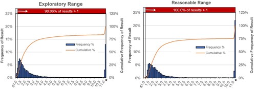
The Monte Carlo analysis with the narrower but more ‘reasonable’ range of input variables more strongly confirmed that the pipeline project was not consistent with the 1.5°C climate goal (Figure 3, right panel). The median emissions significance result was 2.12, and not a single combination of input variables within the 10,000 simulations yielded a result ≤1. This result reflected the heavy influence of operating lifespan, where lower lifespan is more conducive to smaller project impact and higher chance of getting a ‘passing’ score. In this subset analysis, lifespan distribution was limited to a range with minimum value of 10 years rather than 1 year in the exploratory range. Further, despite our generous characterization of a 10-year operating lifespan as ‘reasonable’, it seems highly unlikely that a new build project would be considered so from an economic perspective, given that estimates of economic life used in ratemakings for depreciation typically exceed 20–30 years (Kalen, 2019; Molnar, 2022).

In both Monte Carlo analyses, over 10% of simulation conditions yielded a non-quantitative result of infinity (see Figure 3). These instances reflect a minority of the selected climate scenarios (4 of 18), where committed emissions were estimated to consume the entire climate goal-based carbon budget during the tested operational lifespan of the project.

Finally, we looked to the results of the single factor sensitivity analyses with two major questions in mind: (1) which individual factors, if any, are sensitive enough to tip the scale with respect to the significance conclusion of the climate test for this example project, and (2) are any of them among the most uncertain (e.g. defining the path of committed emissions over time). Ultimately, we found that not all parameters had an effect at all (i.e. capacity factor), and the only one capable of tipping the project from inconsistent to consistent is the project’s operating lifespan due to its powerful effect on how all elements of the climate test components are calculated. Notably none of the uncertain committed emission factors alone, was influential enough to tip the baseline result into a contrary finding of less than significant (≤1). Full results and discussion for the sensitivity analyses can be found in Appendix A-3 and Supplemental Data file SD3.

4.3. Limitations and future work

We plan to pursue several lines of development in following up to this methodological debut. Major themes include scope expansions to continue improving the completeness and accuracy of the climate impact characterization, and the ability of decision support results best inform regulatory choices on fossil fuel infrastructure projects. In the near term, we anticipate creating a version that would allow varying inclusion in the denominator of either narrow sector-specific (oil, gas, or coal) emissions or, alternatively, energy sector-wide emissions, in addition to the current formulation of including all fossil fuel emissions.

One notable limitation of the current tool version is with respect to impacts from GHGs other than CO₂. Currently, the tool assesses only CO₂ emissions in the context of carbon budgets, although those budgets are derived from multi-gas models of limiting warming. Fossil fuel projects also emit other, more potent GHGs, principal among them methane, which have much higher global warming potentials (GWP) than CO₂. Because methane has a shorter residence life in the atmosphere than CO₂, incorporating this gas into the project lifecycle emissions, budgeted emissions, and committed emissions components of the climate test metric will require further development beyond the scope of this initial demonstration. While imperfect, promising paths include use of new so-called micro-climate models, such as ‘GWP*’, which is better suited to use cumulative GHG emissions as a proxy for temperature increases and climate impact (IPCC, 2021a; Smith et al., 2021) or individual gas-based metrics.

Additionally, the current form of the climate test metric presented here was defined for one specific type of application: evaluating U.S.-based, new, fossil energy projects (e.g. oil and gas pipelines, drilling projects, or gas and coal power plants). The default data in the beta workbook tool in SD applies for gas pipelines only, but we also plan to release data for oil projects. We are in the process of an update to expand the tool to international projects, such as infrastructure for LNG exports, which requires selecting the appropriate regional input data for each climate goal and energy system component. In addition to looking at new projects, the metric may also have a use, with some modification, to evaluate existing energy projects; for example, it could be used to inform decisionmakers about the climate impact and implications of early retirement decisions for existing infrastructure or for mitigation policies more broadly targeting the operation of existing fossil energy infrastructure. Further, we could extend the climate test tool to evaluate non-fossil energy projects (such as biomass or renewables) or non-energy projects with climate consequences (such as transportation infrastructure) by redefining the function-normalizing denominator i.e. the fossil energy contribution – to match the scope of the other applications.

While the climate test is sufficiently flexible to address these effects, we do not currently explore any kind of ‘net’ emissions effects, either from substitution of existing sources or possible downstream mitigation (e.g. carbon capture) in these results. The tool’s default use appropriately puts the onus on the proponents, rather than the reviewing agency, to demonstrate that substitution will in fact occur, and if so to what degree, by assuming additivity.

Multiple data sources can be improved upon with additional work. A new and much larger database of 1.5℃ and 2℃ scenario data is available from the IAMC database, and can be integrated into the tool in a new version (Byers et al., 2022). Additionally, committed emission data were based on 2018 assessment of demand-side infrastructure use. Other more recent estimates that use supply-side perspectives instead suggest that committed emissions may already exceed 1.5℃, approaching 2℃ (Trout et al., 2022). Although 1.5℃ with low or no overshoot is clearly the more protective temperature guide, presenting results relative to multiple climate goals may allow for more scenarios where results are useful to decisionmakers.

As a guidepost for ongoing development of the climate test, GHG emissions are not the only climate-related characteristic by which fossil fuel projects can or should be evaluated in decision-making processes to determine approval or continued operation. The economic viability of fossil fuel projects in a decarbonizing world is also a relevant question for regulators and public policy decisionmakers, as well as for investors. We are currently developing a companion analytical tool to evaluate the economic viability of individual fossil fuel projects in the context of their consistency with meeting climate goals. It will also be critical to identify the means to ensure that the climate test is deployed in a manner that does not override environmental justice considerations; environmental justice and local community impacts will need to be considered in a manner integral to, and on par with, the emissions significance metric described in this paper.

On the policy front, climate test results demonstrate the tension between continuing residual demand for fossil fuels and their infrastructure, as shown in modelled pathways for how to meet our climate goals, and the fact that individual fossil fuel projects are almost entirely inconsistent with those goals writ large. To the extent that continuing need or demand for fossil fuel may not be able to be entirely diminished (as indicated by widespread reliance on carbon dioxide removal for harder-to-abate sectors, for example), policies and approval parameters could in principle consider such factors as potential mitigation along the supply chain, and the relative consistency with climate goals of various options and alternatives to meet the need. However as this tension is addressed, the climate test provides important information needed to navigate decisions in the context of individual project approvals.

5. Conclusions

These initial results demonstrate that the climate test analytical method presented here is a viable and robust tool for assessing, interpreting, and comparing the climate impact and significance of individual fossil fuel projects relative to long-term, global decarbonization goals and pathways. Our analysis suggests the test will be immediately suitable to apply to future assessments of proposed new fossil fuel projects in the U.S. legal context. It also indicates the test will provide distinct advantages over current, project specific GHG emissions evaluation methods: superior quantification of all emissions, more informative contextualization of those emissions, and an objective basis for decision-making about their climate significance. Other countries with similar EIA laws and good energy data availability, like Canada, could also readily adopt this methodology by simply swapping out the regional data to reflect their own carbon budgets, fossil demand, emission factors, and committed emissions as input to our model. With further development, the tool can also be adapted for other applications as described in our discussion on future work.

Beyond this, both the process used to develop relevant metrics and the gas pipeline example analysis yielded some key insights worth summarizing here. First, full lifecycle emissions assessment should be a necessary part of climate impact assessment. For fossil fuel projects, where the majority of lifecycle emissions occur during end use combustion that is dependent upon activity during earlier production, processing, and transport stages, it is irresponsible to neglect the potential for these indirect emissions, even if there is potential for substitution to cleaner technologies and processes. Evaluating only direct project emissions in isolation, as has frequently occurred in regulatory agency reviews, is both misleading and inaccurate.

Second, the climate impact of a new fossil energy project can only be meaningfully evaluated in the context of the existing fossil energy system. As our results show, because large fractions of the carbon budget are already committed to (along with the relevant share of future unmet energy demand), the relative impact of a new project is higher than what would be portrayed by simpler comparisons to annual emissions or even a total carbon budget.

Third, comparing the project’s impact in the context of the evolving energy system under climate goal-consistent conditions is far more informative to decisionmakers than static, status quo comparisons. The prior comparisons are fundamentally uninterpretable, and underestimate climate impact by neglecting cumulative effects of existing energy system emissions.

Fourth, the operational timeframe of a project has a large influence on its climate impact. Timeframe defines the analytical scope for all elements of the significance metric, determining the period-relevant emissions constraint (i.e. carbon budget) and the existing energy system variables, all of which will be changing rapidly for decarbonization over the next decades. Our results emphasize the increasingly constrained system that any new fossil energy projects would seek to enter. These results show that only short, and likely uneconomic, project lifespans are potentially consistent with climate goals.

Finally, without an objective decision criterion, there can be no trustworthy basis on which to determine the significance of any given level of climate emissions. Significance as we frame it is a threshold defined by a project’s consistency with published emissions and energy pathways for limiting warming. Our tool is distinct in providing, in addition to emissions impact quantification, a second conceptually integrated and equally dynamic analysis of the project’s contribution to climate-target consistent energy demand. The functionally defined, data-driven decision threshold that results enables the climate test to help reframe project-specific climate analysis in relevant, objective, and rigorous scientific terms, which in turn can help guide nations towards their climate goals.

Acknowledgements

M.B., A.A., and C.S. contributed equally to conceptual development and writing. M.B. designed the metric calculations and led data analysis and interpretation. C.S. and M.B. made graphics. In addition to the anonymous reviewers, the authors would like to Synapse Energy Economics for support in data collection, analysis, and preliminary review of the gas pipeline example – specifically, Dr. Erin Camp, Jon Tabernero, Jackie Litynski, and Dr. Asa Hopkins; early peer reviewers, including Dr. Joelle Labastide, and Dr. Elizabeth Moore, for feedback on previous drafts of this work; Dr. Dawn Woodard and many colleagues from across programmes and functions at NRDC who played a role in laying the foundation, developing, and refining the climate test concept and methodology used in the present analysis, for expert analytical and legal guidance, feedback, and encouragement.

Disclosure statement

No potential conflict of interest was reported by the author(s).

Data availability statement

All data used to support this analysis, as well as a beta version of the climate test tool itself, are available on FigShare at: 10.6084/m9.figshare.19606225.

Notes

1 In this framework, we use carbon budget as shorthand for cumulative emissions under a given warming trajectory. This is distinct from the strict definition.

2 The ‘Production’ and ‘Gathering and Boosting’ stages of gas supply chain lifecycle account for 9.7% of CO₂ emissions from the natural gas supply chain according to NETL’s mean LCA emission factor data, when combustion emission factor from EPA is included as well. Based on this, we chose to use 10% as the baseline value and then vary it as a key parameter in the Monte Carlo and single factor analyses. More on this in Appendix A-1.

References

- 350 Montana v. Haaland, 29 F.4th 1158 (9th Circuit 2022).
- Abaza, H., Bisset, R., & Sadler, B. (2004). Environmental impact assessment and strategic environmental assessment: Towards an integrated approach. UNEP/Earthprint. https://www.iaia.org/pdf/EIA/EIA/CaseStudies/int_ONU_br.pdf
- Achakulwisut, P., Arond, E., Burton, L., Erickson, P., Hocquet, R., Jones, N., Lazarus, M., Cabré, M. M., van Asselt, H., & Vega Araújo, J. A. (2021). The Production Gap Report 2021. https://productiongap.org/2021report/
- BEIS. (2022). Climate compatibility checkpoint design. U.K. Department for Business, Energy & Industrial Strategy. https://www.gov.uk/government/publications/climate-compatibility-checkpoint-design.
- BLM. (2022). Draft supplemental environmental impact statement – Willow master development plan (DOI-BLM-AK-0000-2018-0004-EIS). U.S. Bureau of Land Management. https://eplanning.blm.gov/eplanning-ui/project/109410/510
- Burger, M., & Wentz, J. (2017). Downstream and upstream greenhouse Gas emissions: The proper scope of NEPA review. Harvard Environmental Law Review, 41, 109. https://doi.org/10.2139/ssrn.2748702.
- Byer, P., Cestti, R., Croal, P., Fisher, W., Hazell, S., Kolhoff, A., & Kørnøv, L. (2018). Climate change in impact assessment: International best practice principles. Special publication series No. 8. International Association for Impact Assessment. https://www.iaia.org/uploads/pdf/SP8.pdf.
- Byers, E., Krey, V., Kriegler, E., Riahi, K., Schaeffer, R., Kikstra, J., Lamboll, R., Nicholls, Z., Sandstad, M., Smith, C., van der Wijst, K., Al-Khourdajie, A., Lecocq, F., Portugal-Pereira, J., Saheb, Y., Stromman, A., Winkler, H., Auer, C., Brutschin, E., … van Vuuren, D. (2022). Ar6 scenarios database. Intergovernmental Panel on Climate Change. https://doi.org/10.5281/zenodo.7197970.
- CEQ. (2016). Final guidance for Federal Departments and Agencies on consideration of greenhouse gas emissions and the effects of climate change in National Environmental Policy Act reviews. U.S. Council on Environmental Quality. https://ceq.doe.gov/docs/ceq-regulations-and-guidance/nepa_final_ghg_guidance.pdf.
- CEQ. (2023). National Environmental Policy Act guidance on consideration of greenhouse gas emissions and climate change. Notice CEQ-2022-0005. U.S. Council on Environmental Quality. https://www.federalregister.gov/documents/2023/01/09/2023-00158/national-environmental-policy-act-guidance-on-consideration-of-greenhouse-gas-emissions-and-climate.
- ClimateTest.Org. (2016, February). http://web.archive.org/web/20161201090030/http://www.climatetest.org/.
- DFFE. (2021, June 25). Consultation on intention to publish the national guideline for consideration of climate change implications in applications for environmental authorisations, atmospheric emission licences and waste management licences. South Africa Department of Forestry, Fisheries and Environment in Government Gazette. https://cer.org.za/wp-content/uploads/2021/06/NEMA-Consultation-on-intention-to-publish-the-National-Guideline-for-consideration-of-climate-change-implications-in-applications-for-enviro-authorisations-AELs-and-waste-managemen-1.pdf.
- Doelle, M. (2018). Integrating climate change into environmental impact assessments: Key design elements. SSRN Electronic Journal, January. https://doi.org/10.2139/ssrn.3273499
- EarthLife Africa Johannesburg v Minister of Environmental Affairs and Others. (2017). The High Court of South Africa Gauteng Division, Pretoria. http://climatecasechart.com/wp-content/uploads/sites/16/non-us-case-documents/2017/20170306_Caseno.-6566216_judgment-1.pdf.
- ECCC. (2022, October 4). Draft guidance for best-in-class GHG emissions performance by Oil and Gas projects. Environment and Climate Change Canada. https://www.canada.ca/en/services/environment/weather/climatechange/climate-plan/oil-gas-emissions-cap/best-class-draft-guidance.html.
- EIA. (2019). Monthly energy review April 2019. U.S. Energy Information Administration. https://www.eia.gov/totalenergy/data/monthly/archive/00351904.pdf.
- EPA. (2016). Greenhouse Gas inventory guidance: Direct emissions from stationary combustion sources. United States Environmental Protection Agency Center for Corporate Climate Leadership. https://www.epa.gov/sites/default/files/2016-03/documents/stationaryemissions_3_2016.pdf.
- Erickson, P., & Lazarus, M. (2018). Towards a climate test for industry: Assessing a Gas-based methanol plant. Discussion Brief. Stockholm Environmental Institute. https://www.sei.org/publications/assessing-gas-methanol-plant/.
- FERC. (2019). Final environmental impact statement for the Jordan cove energy project. Environmental Impact Statement FERC/FEIS-0292F. U.S. Federal Energy Regulatory Commission. https://www.ferc.gov/sites/default/files/2020-05/11-15-19-FEIS_Part_1.pdf.
- FERC. (2022). Consideration of greenhouse gas emissions in natural gas infrastructure project reviews. Docket No. PL21-3-000. U.S. Federal Energy Regulatory Commission. https://www.ferc.gov/media/pl21-3-000.
- Hasselman, J., & Erickson, P. (2022, May). NEPA review of fossil fuels projects—Principles for applying a ‘Climate Test’ for new production and infrastructure. https://earthjustice.org/wp-content/uploads/climate_test_-_hasselman_erickson.pdf.
- Hein, J., Schwartz, J., & Zevin, A. (2019). Pipeline approvals and GHG emissions. NYU Institute for Policy Integrity. https://policyintegrity.org/publications/detail/pipeline-approvals-and-greenhouse-gas-emissions.
- High Country Conservation Advocates v. Forest Service, 52 F.Supp.3d *1174 (D.Colo. 2014).
- Huppmann, D., Kriegler, E., Krey, V., Riahi, K., Rogelj, J., Rose, S. K., Weyant, J., Bauer, N., Bertram, C., Bosetti, V., Calvin, K., Doelman, J., Drouet, L., Emmerling, J., Frank, S., Fujimori, S., Gernaat, D., Grubler, A., Guivarch, C., … Zhang, R. (2018). IAMC 1.5°C scenario explorer and data hosted by IIASA. Integrated Assessment Modeling Consortium & International Institute for Applied Systems Analysis, https://doi.org/10.22022/SR15/08-2018.15429
- IEA. (2021). Net Zero by 2050. Paris: International Energy Agency. https://www.iea.org/reports/net-zero-by-2050.
- INGAA. (2019). The interstate natural gas transmission system: Scale, physical complexity and business model. Interstate Natural Gas Association of America. http://www.ingaa.org/file.aspx?id=10751.
- IPCC. (2018). Global warming of 1.5°C. An IPCC special report on the impacts of global warming of 1.5°C above pre-industrial levels and related global greenhouse gas emission pathways, in the context of strengthening the global response to the threat of climate change, sustainable development, and efforts to eradicate poverty. https://www.ipcc.ch/sr15/.
- IPCC. (2021a). Climate change 2021: The physical science basis. Contribution of working group I to the sixth assessment report of the intergovernmental panel on climate change. Cambridge University Press. https://www.ipcc.ch/report/sixth-assessment-report-working-group-i/.
- IPCC. (2021b). Summary for policymakers. In Climate change 2021: The physical science basis. Contribution of working group I to the sixth assessment report of the intergovernmental panel on climate change. Cambridge University Press. https://www.ipcc.ch/report/sixth-assessment-report-working-group-i/.
- Jaccard, M., Hoffele, J., & Jaccard, T. (2018). Global carbon budgets and the viability of new fossil fuel projects. Climatic Change, 150(1), 15–28. https://doi.org/10.1007/s10584-018-2206-2
- Kalen, S. (2019). A bridge to nowhere? Our energy transition and the natural Gas pipeline wars. Michigan Journal of Environmental & Administrative Law, 9, 319. https://doi.org/10.36640/mjeal.9.2.bridge.
- Littlefield, J., Roman-White, S., Augustine, D., Pegallapati, A., Zaimes, G. G., Rai, S., Cooney, G., & Skone, T. J. (2019). Life cycle analysis of natural gas extraction and power generation. DOE/NETL-2019/2039. National Energy Technology Laboratory. https://netl.doe.gov/energy-analysis/details?id=7c7809c2-49ac-4ce0-ac72-3c8f8a4d87ad.
- Marchau, V. A., Walker, W. E., Bloemen, P. J., & Popper, S. W. (2019). Decision making under deep uncertainty: From theory to practice. Springer. https://doi.org/10.1007/978-3-030-05252-2.
- Mayembe, R., Simpson, N. P., Rumble, O., & Norton, M. (2023). Integrating climate change in environmental impact assessment: A review of requirements across 19 EIA regimes. Science of The Total Environment, 869(April), 161850. https://doi.org/10.1016/j.scitotenv.2023.161850
- Molnar, G. (2022). Economics of gas transportation by pipeline and LNG. In M. Hafner & G. Luciani (Eds.), The Palgrave handbook of international energy economics (pp. 23–57). Springer International Publishing. https://doi.org/10.1007/978-3-030-86884-0_2.
- Montana Envt'l Info. Ctr. V. Haaland, 2022 WL 2466794 (D.Mont. 2022). https://casetext.com/case/montenvtl-info-ctr-v-haaland-2.
- Montana Envt'l Info. Ctr. V. Office of Surface Mining, 274 F.Supp.3d 1074 (D.Mont. 2017).
- Noble, D., & Brady, K. (2017). NEB Modernization: Aligning energy project assessment with climate policy. Environment Defence Canada. https://environmentaldefence.ca/report/climate-testaligning- energy-project-assessment-climate-policy/.
- Rogelj, J., Shindell, D., Jiang, K., Fifita, S., Forster, P., Ginzburg, V., Handa, C., Kheshgi, H., Kobayashi, S., Kriegler, E., Mundaca, L., Séférian, R., Vilarino, M. V., Calvin, K., de Oliveira de Portugal Pereira, J. C., Edelenbosch, O., Emmerling, J., Fuss, S., Gasser, T., … Zickfeld, K. (2018). Mitigation pathways compatible with 1.5°C in the context of sustainable development. In Special report on the impacts of global warming of 1.5°C. Intergovernmental Panel on Climate Change. http://www.ipcc.ch/report/sr15/.
- San Juan Citizens Alliance v. BLM, 326 F.Supp.3d 1227 (D.N.M. 2018).
- Sierra Club v. FERC, 867 F.3d 1357 (D.C. Cir. 2017). https://casetext.com/case/sierra-club-v-fed-energyregulatory-commn-1
- Smith, M. A., Cain, M., & Allen, M. R. (2021). Further improvement of warming-equivalent emissions calculation. NPJ Climate and Atmospheric Science, 4(1), 19. https://doi.org/10.1038/s41612-021-00169-8
- Smith, S., & Braathen, N. A. (2015). Monetary carbon values in policy appraisal, no. 92. https://doi.org/10.1787/5jrs8st3ngvh-en.
- Tong, D., Zhang, Q., Zheng, Y., Caldeira, K., Shearer, C., Hong, C., Qin, Y., & Davis, S. J. (2019). Committed emissions from existing energy infrastructure Jeopardize 1.5°C climate target. Nature, 572(7769), 373–377. https://doi.org/10.1038/s41586-019-1008-7
- Trout, K., Muttitt, G., Lafleur, D., Van de Graaf, T., Mendelevitch, R., Mei, L., & Meinshausen, M. (2022). Existing fossil fuel extraction would warm the world beyond 1.5°C. Environmental Research Letters, 17(6), 064010. https://doi.org/10.1088/1748-9326/ac6228
- Utah Physicians for a Healthy Environment v. BLM, 528 F.Supp.3d 1222 (D. Utah 2021). https://www.govinfo.gov/content/pkg/USCOURTS-utd-2_19-cv-00256/pdf/USCOURTS-utd-2_19-cv-00256-0.pdf
- van der Bank, M., & Karsten, J. (2020). Climate change and South Africa: A critical analysis of the Earthlife Africa Johannesburg and Another v Minister of Energy and Others 65662/16 (2017) case and the drive for concrete climate practices. Air, Soil and Water Research, 13. https://doi.org/10.1177/1178622119885372.
- Wildearth Guardians v. Zinke, 368 F. Supp. 3d 41 (D.D.C. 2019).
- Wilderness Workshop v. BLM, 342 F. Supp. 3d 1145 (D. Colo. 2018).
- WORC v. BLM, 2018 WL 1475470 (D. Mont. 2018).
- WRI and WBCSD. (2004). The greenhouse gas protocol: A corporate accounting and reporting standard (Revised Ed.). World Resources Institute and World Business Council for Sustainable Development.