Short-time near-the-money skew in rough fractional volatility models

Abstract

We consider rough stochastic volatility models where the driving noise of volatility has fractional scaling, in the ‘rough’ regime of Hurst parameter $H<1/2$. This regime recently attracted a lot of attention both from the statistical and option pricing point of view. With focus on the latter, we sharpen the large deviation results of Forde-Zhang [Asymptotics for rough stochastic volatility models. SIAM J. Financ. Math., 2017, 8(1), 114–145] in a way that allows us to zoom-in around the money while maintaining full analytical tractability. More precisely, this amounts to proving higher order moderate deviation estimates, only recently introduced in the option pricing context. This in turn allows us to push the applicability range of known at-the-money skew approximation formulae from CLT type log-moneyness deviations of order $t^{1/2}$ (works of Alòs, León & Vives and Fukasawa) to the wider moderate deviations regime.

Keywords:

• Rough stochastic volatility model
• European option pricing
• Small-time asymptotics
• Moderate deviations

2010 Mathematics Subject Classification:

• 91G20
• 60H30
• 60F10
• 60H07
• 60G22
• 60G18

1. Introduction

Since the groundbreaking work of Gatheral et al. (2014), the past two years have brought about a gradual shift in volatility modeling, leading away from classical diffusive stochastic volatility models towards so-called rough volatility models. The term was coined in Gatheral et al. (2014) and Bayer et al. (2016), and it essentially describes a family of (continuous-path) stochastic volatility models where the driving noise of the volatility process has Hölder regularity lower than Brownian motion, typically achieved by modeling the fundamental noise innovations of the volatility process as a fractional Brownian motion with Hurst exponent (and hence Hölder regularity) $H<1/2$. Here, we would also like to mention pioneering work on asymptotics for rough volatility models in Alòs et al. (2007) and Fukasawa (2011). A major appeal of such rough volatility models lies in the fact that they effectively capture several stylized facts of financial markets both from a statistical (Gatheral et al. 2014; Bennedsen et al. 2016) and an option-pricing point of view (Bayer et al. 2016). In particular, with regards to the latter point of view, a widely observed empirical phenomenon in equity markets is the ‘steepness of the smile on the short end’ describing the fact that as time to maturity becomes small the empirical implied volatility skew follows a power law with negative exponent, and thus becomes arbitrarily large near zero. While standard stochastic volatility models with continuous paths struggle to capture this phenomenon, predicting instead a constant at-the-money implied volatility behavior on the short end (Gatheral 2011), models in the fractional stochastic volatility family (and more specifically so-called rough volatility models) constitute a class, well-tailored to fit empirical implied volatilities for short dated options.

Typically, the popularity of asset pricing models hinges on the availability of efficient numerical pricing methods. In the case of diffusions, these include Monte Carlo estimators, PDE discretization schemes, asymptotic expansions and transform methods. With fractional Brownian motion being the prime example of a process beyond the semimartingale framework, most currently prevalent option pricing methods – particularly the ones assuming semimartingality or Markovianity – may not easily carry over to the rough setting. In fact, the memory property (aka non-Markovianity) of fractional Brownian motion rules out PDE methods, heat kernel methods and all related methods involving a Feynman-Kac-type Ansatz. Previous work has thus focused on finding efficient Monte Carlo simulation schemes (Bayer et al. 2016; Bennedsen et al. 2017; Bayer et al. 2017) or – in the special case of the Rough Heston model – on an explicit formula for the characteristic function of the log-price (see El Euch and Rosenbaum 2016), thus in this particular model making pricing amenable to Fourier based methods. In our work, we rely on small-maturity approximations of option prices. This is a well-studied topic for which we mention (with no claim to completeness) a number of works, either based on large deviations or central limit type scaling regime, that inspired this work: Alòs et al. (2007), Fukasawa (2011), Deuschel et al. (2014a), Deuschel et al. (2014b) and Fukasawa (2017), also Medvedev and Scaillet (2003, 2007), Osajima (2007, 2015), Guennoun et al. (2014), Mijatović and Tankov (2016) and especially Forde and Zhang (2017). Rather recently, Friz et al. (2018) introduced another regime called moderately-out-of-the-money (MOTM), which, in a sense, effectively navigates between the two regimes mentioned above, by rescaling the strike with respect to the time to maturity. This approach has various advantages. On the one hand, it reflects the market reality that as time to maturity approaches zero, strikes with acceptable bid-ask spreads tend to move closer to the money (see Friz et al. 2018 for more details). On the other hand, it allows us to zoom in on the term structure of implied volatility around the money at a high resolution scale. To be more specific, our paper adds to the existing literature in two ways. First, we obtain a generalization of the Osajima energy expansion (Osajima 2015) to a non-Markovian case, and using the new expansion, we extend the analysis of Friz et al. (2018) to the case, where the volatility is driven by a rough $(H<1/2)$ fractional Brownian motion. Indeed, Laplace approximation methods on Wiener space in the spirit of Azencott (1982, 1985), Ben Arous (1988) and Bismut (1984) can be adapted to the present context, so that our analysis builds upon this framework in a fractional setting. Unlike many other works in this field, we do not rely on density expansions. Finally, using a version of the ‘rough Bergomi model’ (Bayer et al. 2016), we demonstrate numerically that our implied volatility asymptotics capture very well the geometry of the term structure of implied volatility over a wide array of maturities, extending up to a year.

The paper is organized as follows: In Section 2 we set the scene, describing the class of models included in our framework ((1(1) $\frac{\mathrm{d}{S}_t}{S_t}=\sigma \left({\hat{B}}_t\right)\mathrm{d}\left(\overline{\rho }{W}_t+\rho B_t\right).$(1) ) and (2(2) ${\hat{B}}_t={\int }_0^{t}K\left(t,s\right)\mathrm{d}{B}_s,t\ge 0,$(2) )) and recalling some known results ((4(4) $\begin{array}{ll}\frac{1}{2}{∥h∥}_{H_0^1}^2+\frac{1}{2}{∥f∥}_{H_0^1}^2,& f,h\in H_0^1\mathrm{and}\hat{f}=K\dot{f},\\ +\mathrm{\infty },& \mathrm{otherwise},\end{array}$(4) ) and (7(7) $\begin{array}{rl}I\left(x\right)& =\underset{h,f\in H_0^1}{inf}\left\{\frac{1}{2}{\int }_0^1{\dot{h}}^2\mathrm{d}t+\frac{1}{2}{\int }_0^1{\dot{f}}^2\mathrm{d}t:{\varphi }_1\left(h,f\right)=x\right\}\\ & =\underset{f\in H_0^1}{inf}\left\{\frac{1}{2}\frac{{\left(x-\rho ⟨\sigma \left(\hat{f}\right),\dot{f}⟩\right)}^2}{{\overline{\rho }}^2⟨{\sigma }^2\left(\hat{f}\right),1⟩}+\frac{1}{2}{\int }_0^1{\dot{f}}^2\mathrm{d}t\right\},\end{array}$(7) )), which are the starting point of our analysis. Most importantly, we argue that for small-time considerations it would suffice to restrict our attention to a class of stochastic volatility models of the form (3(3) $\mathrm{d}{X}_t=-\frac{1}{2}{\sigma }^2\left({\hat{B}}_t\right)\mathrm{d}t+\sigma \left({\hat{B}}_t\right)\mathrm{d}\left(\overline{\rho }W+\rho B\right),X_0=0.$(3) ) with a volatility process driven by a Gaussian Volterra process such as in (2(2) ${\hat{B}}_t={\int }_0^{t}K\left(t,s\right)\mathrm{d}{B}_s,t\ge 0,$(2) ). We formulate general assumptions on the Volterra kernel (Assumptions 2.1 and 2.5) and on the function σ in (3(3) $\mathrm{d}{X}_t=-\frac{1}{2}{\sigma }^2\left({\hat{B}}_t\right)\mathrm{d}t+\sigma \left({\hat{B}}_t\right)\mathrm{d}\left(\overline{\rho }W+\rho B\right),X_0=0.$(3) ) (Assumption 2.4) under which our results are valid. In Section 3 we gather our main results, concerning a higher order expansion of the energy (Theorem 3.1), and a general expansion formula for the corresponding call prices. We derive the classical Black-Scholes expansion for the call price, using the latter result mentioned above. In addition, in Section 3 we formulate moderate deviation expansions, which allow us to derive the corresponding asymptotic formulae for implied volatilities and implied volatility skews. Finally, Section 4 displays our simulation results. Sections 5–7 are devoted to proofs of the energy expansion, the price expansion and the moderate deviations expansion, respectively. In the appendix, we have collected some auxiliary lemmas, which are used in different sections.

2. Exposition and assumptions

We consider a rough stochastic volatility model, normalized to r=0 and $S_0=1$, of the form suggested by Forde and Zhang (2017) (1) $\frac{\mathrm{d}{S}_t}{S_t}=\sigma \left({\hat{B}}_t\right)\mathrm{d}\left(\overline{\rho }{W}_t+\rho B_t\right).$(1) Here $(W,B)$ are two independent standard Brownian motions, $\rho \in (-1,1)$ a correlation parameter, and ${\overline{\rho }}^2=1-{\rho }^2$. Then $\overline{\rho }W+\rho B$ is another standard Brownian motion which has constant correlation ρ with the factor B, which drives the stochastic volatility ${\sigma }_{\mathrm{stoch}}\left(t,\omega \right):=\sigma \left({\hat{B}}_t\left(\omega \right)\right)\equiv \sigma \left(\hat{B}\right).$ Here $\sigma (.)$ is some real-valued function, typically smooth but not bounded, and we will denote by ${\sigma }_0:=\sigma \left(0\right)$ the spot volatility, with $\hat{B}$ a Gaussian (Volterra) process of the form (2) ${\hat{B}}_t={\int }_0^{t}K\left(t,s\right)\mathrm{d}{B}_s,t\ge 0,$(2) for some kernel K, which shall be further specified in Assumptions 2.1 and 2.5 below. The log-price $X_t=\log \left(S_t\right)$ satisfies (3) $\mathrm{d}{X}_t=-\frac{1}{2}{\sigma }^2\left({\hat{B}}_t\right)\mathrm{d}t+\sigma \left({\hat{B}}_t\right)\mathrm{d}\left(\overline{\rho }W+\rho B\right),X_0=0.$(3) Recall that by Brownian scaling, for fixed t>0, $(B_{ts},W_{ts}{)}_{s\ge 0}\stackrel{law}{=}\epsilon (B_s,W_s{)}_{s\ge 0},\mathrm{where}\epsilon \equiv \epsilon \left(t\right)\equiv t^{1/2}.$ As a direct consequence, classical short-time SDE problems can be analyzed as small-noise problems on a unit time horizon. For our analysis, it will also be crucial to impose such a scaling property on the Gaussian process $\hat{B}$ (more precisely, on the kernel K in (2(2) ${\hat{B}}_t={\int }_0^{t}K\left(t,s\right)\mathrm{d}{B}_s,t\ge 0,$(2) )) driving the volatility process in our model:

Assumption 2.1

Small time self-similarity

There exists a number $t_0$ with $0<t_0\le 1$ and a function $t\mapsto \hat{\epsilon }=\hat{\epsilon }\left(t\right),$ $0\le t\le t_0,$ such that $({\hat{B}}_{ts}:0\le s\le t_0)\stackrel{law}{=}(\hat{\epsilon }{\hat{B}}_s:0\le s\le t_0).$

In fact, we will always have $\hat{\epsilon }\equiv \hat{\epsilon }\left(t\right)\equiv t^H={\epsilon }^{2H},$ which covers the examples of interest, in particular standard fractional Brownian motion $\hat{B}=B^H$ or Riemann-Liouville fBM with explicit kernel $K(t,s)=\sqrt{2H}{∣t-s∣}^{H-1/2}$. (This is very natural, even from a general perspective of self-similar processes, see Lamperti 1962.)

We insist that no (global) self-similarity of $\hat{B}$ is required, as only $\hat{B}{|}_{[0,t]}$ for arbitrarily small t matters.

Remark 2.2

It should be possible to replace the fractional Brownian motion by a certain fractional Ornstein-Uhlenbeck process in the results obtained in this paper. Intuitively, this replacement creates a negligible perturbation (for $t\ll 1$) of the fBm environment. A similar situation was in fact encountered in Cass and Friz (2010), where fractional scaling at times near zero was important. To quantify the perturbation, the authors of Cass and Friz (2010) introduced an easy to verify coupling condition (see Corollary 2 in Cass and Friz 2010). It should be possible to employ a version of this condition in the present paper to justify the replacement mentioned above. We will however not pursue this point further here.

Remark 2.3

Throughout this article, one can consider a classical (Markovian, diffusion) stochastic volatility setting by taking $K\equiv 1$, or equivalently $H\equiv 1/2$, by simply ignoring all hats ( $\hat{\cdot }$ ) in the sequel. In particular then, $\hat{\epsilon }/\epsilon \equiv 1$ in all subsequent formulae.

General facts on large deviations of Gaussian measures on Banach spaces (Deuschel and Stroock 1989) such as the path space $C\left(\right[0,1],{\mathbb{R}}^3)$ imply that a large deviation principle holds for the triple $\left\{\hat{\epsilon }\right(W,B,\hat{B}):\hat{\epsilon }>0\}$, with speed ${\hat{\epsilon }}^2$ and rate function (4) $\begin{array}{ll}\frac{1}{2}{∥h∥}_{H_0^1}^2+\frac{1}{2}{∥f∥}_{H_0^1}^2,& f,h\in H_0^1\mathrm{and}\hat{f}=K\dot{f},\\ +\mathrm{\infty },& \mathrm{otherwise},\end{array}$(4) where $K\dot{f}\left(t\right):={\int }_0^{t}K\left(t,s\right)\dot{f}\left(s\right)\mathrm{d}s$ for $f\in H_0^1$, the space of absolutely continuous paths with $L^2$ derivative (5) $\begin{array}{rl}& H_0^1:=\left\{f:[0,1]\to \mathbb{R}\mathrm{continuous}\left|{∥f∥}_{H_0^1}^2\right.\right.\\ & \left.:={\int }_0^1{∣\dot{f}\left(s\right)∣}^2\mathrm{d}s<\mathrm{\infty },f\left(0\right)=0\right\}.\end{array}$(5) This enables us to derive a large deviations principle for X in (3(3) $\mathrm{d}{X}_t=-\frac{1}{2}{\sigma }^2\left({\hat{B}}_t\right)\mathrm{d}t+\sigma \left({\hat{B}}_t\right)\mathrm{d}\left(\overline{\rho }W+\rho B\right),X_0=0.$(3) ): the (local) small-time self-similarity property of $\hat{B}$ (Assumption 2.1) implies that $X_t\stackrel{law}{=}{X}_1^{\epsilon }$ where $\mathrm{d}{X}_t^{\epsilon }=\sigma \left(\hat{\epsilon }{\hat{B}}_t\right)\epsilon \mathrm{d}\left(\overline{\rho }{W}_t+\rho B_t\right)-\frac{1}{2}{\epsilon }^2{\sigma }^2\left(\hat{\epsilon }{\hat{B}}_t\right)\mathrm{d}t,X_0^{\epsilon }=0.$ For what follows, it will be convenient to consider a rescaled version of (3(3) $\mathrm{d}{X}_t=-\frac{1}{2}{\sigma }^2\left({\hat{B}}_t\right)\mathrm{d}t+\sigma \left({\hat{B}}_t\right)\mathrm{d}\left(\overline{\rho }W+\rho B\right),X_0=0.$(3) ) $\begin{array}{rl}& \mathrm{d}{\hat{X}}_t^{\epsilon }\equiv \mathrm{d}\left(\frac{\hat{\epsilon }}{\epsilon }{X}_t^{\epsilon }\right)=\sigma \left(\hat{\epsilon }{\hat{B}}_t\right)\hat{\epsilon }\mathrm{d}\left(\overline{\rho }{W}_t+\rho B_t\right)\\ & -\frac{1}{2}\epsilon \hat{\epsilon }{\sigma }^2\left(\hat{\epsilon }{\hat{B}}_t\right)\mathrm{d}t,{\hat{X}}_0^{\epsilon }=0.\end{array}$ Under a linear growth condition on the function σ, Forde and Zhang (2017) use the extended contraction principle to establish a large deviations principle for (${\hat{X}}_1^{\epsilon }$) with speed ${\hat{\epsilon }}^2$. More precisely, with (6) ${\varphi }_1\left(h,f\right):={\mathrm{\Phi }}_1(h,f,\hat{f})={\int }_0^1\sigma \left(\hat{f}\right)\mathrm{d}\left(\overline{\rho }h+\rho f\right),$(6) the rate function is given by (7) $\begin{array}{rl}I\left(x\right)& =\underset{h,f\in H_0^1}{inf}\left\{\frac{1}{2}{\int }_0^1{\dot{h}}^2\mathrm{d}t+\frac{1}{2}{\int }_0^1{\dot{f}}^2\mathrm{d}t:{\varphi }_1\left(h,f\right)=x\right\}\\ & =\underset{f\in H_0^1}{inf}\left\{\frac{1}{2}\frac{{\left(x-\rho ⟨\sigma \left(\hat{f}\right),\dot{f}⟩\right)}^2}{{\overline{\rho }}^2⟨{\sigma }^2\left(\hat{f}\right),1⟩}+\frac{1}{2}{\int }_0^1{\dot{f}}^2\mathrm{d}t\right\},\end{array}$(7) where $⟨\cdot ,\cdot ⟩$ denotes the inner product on $L^2\left(\right[0,1],dt)$. Several other proofs (under varying assumptions on σ) have appeared since (Jacquier et al. 2017; Bayer et al. 2017; Gulisashvili 2017).

As a matter of fact, this paper relies on moderate – rather than large – deviations, as emphasized in (iiic) below. To this end, let us make

Assumption 2.4

1. $($Positive spot vol$)$ Assume $\sigma :\mathbb{R}\to \mathbb{R}$ is smooth with ${\sigma }_0:=\sigma \left(0\right)>0$.

2. $($Roughness$)$ The Hurst parameter H satisfies $H\in (0,1/2]$.

3. $($Martingality$)$ The price process $S=\exp X$ is a martingale.

4. $($Short-time moments$)$ $\mathrm{\forall }m<\mathrm{\infty }\mathrm{\exists }t>0:E\left(S_t^m\right)<\mathrm{\infty }$.

While condition (iiia) hardly needs justification, we emphasize that conditions (iiia-b) are only used to the extent that they imply condition (iiic) given below (which thus may replace (iiia-b) as an alternative, if more technical, assumption). The reason we point this out explicitly is that all the conditions (iiia-c) are implicit (growth) conditions on the function $\sigma (.)$. For instance, (iiia-b) was seen to hold under a linear growth assumption (Forde and Zhang 2017; Gulisashvili 2017), whereas the log-normal volatility case (think of $\sigma \left(x\right)={\mathrm{e}}^x$) is complicated. Martingality, for instance, requires $\rho \le 0$ and there is a critical moment $m^{\ast }=m^{\ast }\left(\rho \right)$, even when $\rho <0$. See Sin (1998), Jourdain (2004) and Lions and Musiela (2007) for the case $H=1/2$ and the forthcoming work (Friz and Gassiat 2018) for the general rough case $H\in (0,1]$. We view (iiic) simply as a more flexible condition that can hold in situations where (iiib) fails.

1. (Call price upper moderate deviation bound) For every $\beta \in (0,H)$, and every fixed x>0, and ${\hat{x}}_{\epsilon }:=x{\epsilon }^{1-2H+2\beta }$, $E\left[\right({\mathrm{e}}^{X_1^{\epsilon }}-{\mathrm{e}}^{{\hat{x}}_{\epsilon }}{)}^{+}]\le \exp \left(-\frac{x^2+o\left(1\right)}{2{\sigma }_0^2{\epsilon }^{4H-4\beta }}\right).$

This condition is reminiscent of the ‘upper part’ of the large deviation estimate obtained in Forde and Zhang (2017) (8) $E\left[\right({\mathrm{e}}^{X_1^{\epsilon }}-{\mathrm{e}}^{x{\epsilon }^{1-2H}}{)}^{+}]=\exp \left(-\frac{I\left(x\right)+o\left(1\right)}{{\epsilon }^{4H}}\right).$(8) If fact, if one formally applies this with x replaced by $x{\epsilon }^{2\beta }$, followed by Taylor expanding the rate function, $I\left(x{\epsilon }^{2\beta }\right)\sim \frac{1}{2}{I}^{″}\left(0\right)x^2{\epsilon }^{4\beta }=\frac{1}{2{\sigma }_0^2}{x}^2{\epsilon }^{4\beta },$ one readily arrives at the estimate (iiic). Unfortunately, $o\left(1\right)=o_x\left(1\right)$ in (8(8) $E\left[\right({\mathrm{e}}^{X_1^{\epsilon }}-{\mathrm{e}}^{x{\epsilon }^{1-2H}}{)}^{+}]=\exp \left(-\frac{I\left(x\right)+o\left(1\right)}{{\epsilon }^{4H}}\right).$(8) ), which is a serious obstacle in making this argument rigorous. Instead, we will give a direct argument (Lemma 7.1) to see how (iiia-b) implies (iiic).

In the sequel, we will use another mild assumption on the kernel.

Assumption 2.5

The kernel K has the following properties

1. ${\hat{B}}_t={\int }_0^{t}K(t,s)\mathrm{d}{B}_s$ has a continuous $($in $t)$ version on $[0,1]$.

2. $\mathrm{\forall }t\in [0,1]:{\int }_0^{t}K(t,s{)}^2\mathrm{d}s<\mathrm{\infty }$.

Note that the Riemann-Liouville kernel $K(t,s)=\sqrt{2H}(t-s{)}^{\gamma }$, $\gamma =H-1/2$ satisfies Assumption 2.5.

Remark 2.6

Assumption 2.5 implies that the Cameron-Martin space $\mathcal{H}$ of $\hat{B}$ is given by the image of $H_0^1$ under K, i.e. $\mathcal{H}=\{K\dot{f}\mid f\in H_0^1\}.$ See Lemma 5.3 and Remark 5.4 for more details. A reference and also a sufficient condition for Assumption 2.5 (i) can be found e.g. in Decreusefond (2005, Section 3).

3. Main results

The following result can be seen as a non-Markovian extension of work by Osajima (2015). The statement here is a combination of Theorem 5.10 and Proposition (5.14) below. Recall that ${\sigma }_0=\sigma \left(0\right)$ represents spot-volatility. We also set ${\sigma }_0^{\mathrm{\prime }}\equiv {\sigma }^{\mathrm{\prime }}\left(0\right)$.

Theorem 3.1

Energy expansion

The rate function $($or energy$)$ I in (7(7) $\begin{array}{rl}I\left(x\right)& =\underset{h,f\in H_0^1}{inf}\left\{\frac{1}{2}{\int }_0^1{\dot{h}}^2\mathrm{d}t+\frac{1}{2}{\int }_0^1{\dot{f}}^2\mathrm{d}t:{\varphi }_1\left(h,f\right)=x\right\}\\ & =\underset{f\in H_0^1}{inf}\left\{\frac{1}{2}\frac{{\left(x-\rho ⟨\sigma \left(\hat{f}\right),\dot{f}⟩\right)}^2}{{\overline{\rho }}^2⟨{\sigma }^2\left(\hat{f}\right),1⟩}+\frac{1}{2}{\int }_0^1{\dot{f}}^2\mathrm{d}t\right\},\end{array}$(7) ) is smooth in a neighborhood of x=0 $($at-the-money$)$ and it is of the form $I\left(x\right)=\frac{1}{{\sigma }_0^2}\frac{x^2}{2}-\left(6\rho \frac{{\sigma }_0^{\mathrm{\prime }}}{{\sigma }_0^4}{\int }_0^1{\int }_0^{t}K(t,s)\mathrm{d}s\mathrm{d}t\right)\frac{x^3}{3!}+\mathcal{O}\left(x^4\right).$

The next result is an exact representation of call prices, valid in a non-Markovian generality, and amenable to moderate- and large-deviation analysis (Theorem 3.4 below).

Theorem 3.2

Pricing formula

For a fixed log-strike $x\ge 0$ and time to maturity $t>0,$ set $\hat{x}:=\left(\epsilon /\hat{\epsilon }\right)x,$ where $\epsilon =t^{1/2}$ and $\hat{\epsilon }=t^H={\epsilon }^{2H},$ as before. Then we have (9) $\begin{array}{rl}c(\hat{x},t)& =E\left[{\left(\exp \left(X_t\right)-\exp \hat{x}\right)}^{+}\right]\\ & ={\mathrm{e}}^{-I\left(x\right)/{\hat{\epsilon }}^2}{\mathrm{e}}^{\epsilon /\hat{\epsilon }x}J\left(\epsilon ,x\right),\end{array}$(9) where $J\left(\epsilon ,x\right):=E\left[{\mathrm{e}}^{-\left(I^{\mathrm{\prime }}\left(x\right)/{\hat{\epsilon }}^2\right){\hat{U}}^{\epsilon }}\left(\exp \left(\frac{\epsilon }{\hat{\epsilon }}{\hat{U}}^{\epsilon }\right)-1\right){\mathrm{e}}^{I^{\mathrm{\prime }}\left(x\right)R_2^{\epsilon }}{\mathbf{1}}_{{\hat{U}}^{\epsilon }\ge 0}\right]$ and ${\hat{U}}^{\epsilon }$ is a random variable of the form (10) ${\hat{U}}^{\epsilon }=\hat{\epsilon }{g}_1+{\hat{\epsilon }}^2{R}_2^{\epsilon }$(10) with $g_1$ a centred Gaussian random variable, explicitly given in equation (38(38) $g_1={\int }_0^1\left\{\sigma \right({\hat{f}}_t)\mathrm{d}\left(\overline{\rho }{W}_t+\rho B_t\right)+{\sigma }^{\mathrm{\prime }}({\hat{f}}_t\left){\hat{B}}_t\mathrm{d}\left(\overline{\rho }{h}_t+\rho f_t\right)\right\},$(38) ) below, and $R_2^{\epsilon }$ is a $($random$)$ remainder term, in the sense of a stochastic Taylor expansion in $\hat{\epsilon },$ see Lemma 6.2 for more details.

Example 3.3

Black-Scholes model

We fix volatility $\sigma (\cdot )\equiv \sigma >0$, and $H=1/2$ so that $\hat{\epsilon }=\epsilon$ and all $\hat{\cdot }$ can be omitted. Energy is given by $I\left(x\right)=x^2/2{\sigma }^2$ and $U^{\epsilon }=\epsilon g_1+{\epsilon }^2{R}_2^{\epsilon }\equiv \epsilon \sigma W_1-{\epsilon }^2{\sigma }^2/2$ with $R_2^{\epsilon }=R_2\equiv -{\sigma }^2/2$ independent of ϵ. Moreover, (11) $\begin{array}{rl}J\left(\epsilon ,x\right)& =E\left[{\mathrm{e}}^{-\left(I^{\mathrm{\prime }}\left(x\right)/{\epsilon }^2\right)U^{\epsilon }}\left({\mathrm{e}}^{U^{\epsilon }}-1\right){\mathrm{e}}^{I^{\mathrm{\prime }}\left(x\right)R_2}{\mathbf{1}}_{U^{\epsilon }\ge 0}\right]\\ & =E\left[{\mathrm{e}}^{-\left(I^{\mathrm{\prime }}\left(x\right)/\epsilon \right)g_1}\left({\mathrm{e}}^{\epsilon g_1-{\epsilon }^2{\sigma }^2/2}-1\right){\mathbf{1}}_{\{g_1\ge \epsilon {\sigma }^2/2\}}\right]\\ & =E\left[{\mathrm{e}}^{-\alpha W_1}\left({\mathrm{e}}^{\epsilon \sigma W_1-(\epsilon \sigma {)}^2/2}-1\right){\mathbf{1}}_{\{W_1\ge \epsilon \sigma /2\}}\right]\\ & ={\mathrm{e}}^{-(\epsilon \sigma {)}^2/2}M\left(-\alpha +\epsilon \sigma \right)-M\left(-\alpha \right)\end{array}$(11) with $\alpha :=I^{\mathrm{\prime }}\left(x\right)\sigma /\epsilon =\left(1/\sigma \right)\left(x/\epsilon \right)$, and, in terms of the standard Gaussian cdf Φ, $M\left(\beta \right):=E\left[{\mathrm{e}}^{\beta W_1}{\mathbf{1}}_{\{W_1\ge \epsilon \sigma /2\}}\right]={\mathrm{e}}^{{\beta }^2/2}\mathrm{\Phi }\left(\beta -\frac{\epsilon \sigma }{2}\right).$ Using the expansion $\mathrm{\Phi }(-y)=\left(1/y\sqrt{2\pi }\right){\mathrm{e}}^{-y^2/2}(1-y^{-2}+\cdots )$, as $y\to \mathrm{\infty }$ one deduces, for fixed x>0, the asymptotic relation, as $\epsilon \to 0$, (12) $J\left(\epsilon ,x\right)\sim \frac{{\mathrm{e}}^{-x/2}}{\sqrt{2\pi }}\frac{{\epsilon }^3{\sigma }^3}{x^2}.$(12) We will be interested (cf. Theorem 3.4) in replacing x by $\tilde{x}=x{\epsilon }^{2\beta }\to 0$ for $\beta >0$. This gives $\tilde{\alpha }=\left(1/\sigma \right)\left(x/{\epsilon }^{1-2\beta }\right)$ and the above analysis, now based on $\tilde{\alpha }\to \mathrm{\infty }$, remains valid¹ for β in the ‘moderate’ regime $\beta \in [0,1/2)$ and we obtain (13) $\mathrm{\forall }x>0,\beta \in [0,1/2):J\left(\epsilon ,x{\epsilon }^{2\beta }\right)\sim \frac{1}{\sqrt{2\pi }}\frac{{\epsilon }^{3-4\beta }{\sigma }^3}{x^2}.$(13) Let us point out, for the sake of completeness, that a similar expansion is not valid for $\beta >1/2$. To see this, first note that (9(9) $\begin{array}{rl}c(\hat{x},t)& =E\left[{\left(\exp \left(X_t\right)-\exp \hat{x}\right)}^{+}\right]\\ & ={\mathrm{e}}^{-I\left(x\right)/{\hat{\epsilon }}^2}{\mathrm{e}}^{\epsilon /\hat{\epsilon }x}J\left(\epsilon ,x\right),\end{array}$(9) ) implies that $J(\epsilon ,x){|}_{x=0}$ is precisely the ATM call price with time $t={\epsilon }^2$ from expiration. Well-known ATM asymptotics then imply that $J(\epsilon ,x){|}_{x=0}\sim \left(1/\sqrt{2\pi }\right)\epsilon \sigma$ as $\epsilon \to 0$. These asymptotics are unchanged in case of $o\left(t^{1/2}\right)=o\left(\epsilon \right)$ out-of-moneyness (‘almost-at-the-money’ in the terminology of Friz et al. 2018), which readily implies $\mathrm{\forall }x>0,\beta >1/2:J\left(\epsilon ,x{\epsilon }^{2\beta }\right)\sim \frac{1}{\sqrt{2\pi }}\epsilon \sigma =\mathrm{const}\times \epsilon$ At last, we have the borderline case $\beta =1/2$, or $\tilde{x}=x\epsilon$. From e.g. Muhle-Karbe and Nutz (2011, Theorem 3.1), we see that $c(x\epsilon ,{\epsilon }^2)\sim a(x;\sigma )\epsilon$ with positive constant $a(x;\sigma )$. A look at (9(9) $\begin{array}{rl}c(\hat{x},t)& =E\left[{\left(\exp \left(X_t\right)-\exp \hat{x}\right)}^{+}\right]\\ & ={\mathrm{e}}^{-I\left(x\right)/{\hat{\epsilon }}^2}{\mathrm{e}}^{\epsilon /\hat{\epsilon }x}J\left(\epsilon ,x\right),\end{array}$(9) ) then reveals $\mathrm{\forall }x>0:J\left(\epsilon ,x\epsilon \right)\sim a(x;\sigma )\epsilon {\mathrm{e}}^{x^2/2{\sigma }^2}=\mathrm{const}\times \epsilon .$ For the call price expansion in the large / moderate deviations regime, $\beta \in [0,1/2)$, the polynomial in ϵ-behavior of (13(13) $\mathrm{\forall }x>0,\beta \in [0,1/2):J\left(\epsilon ,x{\epsilon }^{2\beta }\right)\sim \frac{1}{\sqrt{2\pi }}\frac{{\epsilon }^{3-4\beta }{\sigma }^3}{x^2}.$(13) ) implies that the J-term in the pricing formula will be negligible on the moderate / large deviation scale, in the sense for any $\theta >0$, we have ${\epsilon }^{\theta }\log J(\epsilon ,x{\epsilon }^{2\beta })\to 0$ as $\epsilon \to 0$. Consequently, with $k_t=k{t}^{\beta }$, for $t={\epsilon }^2$, k>0, $\beta \in [0,1/2)$, we get the ‘moderate’ Black-Scholes call price expansion, $-\log c_{BS}(k_t,t)=\frac{1}{t^{1-2\beta }}\frac{k^2}{2{\sigma }^2}\left(1+o\left(1\right)\right)\mathrm{as}t\downarrow 0.$

While the above can be confirmed by elementary analysis of the Black–Scholes formula, the following theorem exhibits it as an instance of a general principle. See Friz et al. (2018) for a general diffusion statement.

Theorem 3.4

Moderate Deviations

In the rough volatility regime $H\in (0,1/2],$ consider log-strikes of the form $k_t=k{t}^{1/2-H+\beta }\mathrm{for}\mathrm{a}\mathrm{constant}k\ge 0.$ (i) For $\beta \in (0,H),$ and every $\theta >0,$ we have $-\log c(k_t,t)=\frac{I^{\mathrm{\prime \prime }}\left(0\right)}{t^{2H-2\beta }}\frac{k^2}{2}+O\left(t^{3\beta -2H}\right)+O\left(t^{-\theta }\right)\mathrm{as}t\downarrow 0.$ (ii) For $\beta \in (0,\frac{2}{3}H),$ and every $\theta >0,$ we have $\begin{array}{rl}& -\log c(k_t,t)=\frac{I^{\mathrm{\prime \prime }}\left(0\right)}{t^{2H-2\beta }}\frac{k^2}{2}+\frac{I^{\mathrm{\prime \prime \prime }}\left(0\right)}{t^{2H-3\beta }}\frac{k^3}{6}+O\left(t^{4\beta -2H}\right)\\ & +O\left(t^{-\theta }\right)\mathrm{as}t\downarrow 0.\end{array}$ Moreover, $\begin{array}{rl}{I}^{\mathrm{\prime \prime }}\left(0\right)& =\frac{1}{{\sigma }_0^2},\\ I^{\mathrm{\prime \prime \prime }}\left(0\right)& =-6\rho \frac{{\sigma }_0^{\mathrm{\prime }}}{{\sigma }_0^4}{\int }_0^1{\int }_0^{t}K(t,s)\mathrm{d}s\mathrm{d}t=-6\rho \frac{{\sigma }_0^{\mathrm{\prime }}}{{\sigma }_0^4}⟨K1,1⟩,\end{array}$ where $⟨\cdot ,\cdot ⟩$ is the inner product in $L^2\left(\right[0,1\left]\right)$.

Remark 3.5

In principle, further terms (of order $t^{i\beta -2H}$, $i=4,5,\dots$) can be added to this expansion of log call prices, given that the energy has sufficient regularity, see Theorem 3.6. We also note that, for small enough β, the error term $O\left(t^{-\theta }\right)$ can be omitted. In any case, one can replace the additive error bounds by (cruder) ones, where the right-most term in the expansion is multiplied with $(1+o(1\left)\right)$, as was done in Friz et al. (2018).

Proof of Theorem 3.4

We apply Theorem 3.2 with $\hat{x}=k_t=k{t}^{1/2-H+\beta }$, i.e. with $x=k{t}^{\beta }=k{\epsilon }^{2\beta }$. In particular, we so get, with $\hat{\epsilon }=t^H$ and $\epsilon =t^{1/2}$, $c(k_t,t)={\mathrm{e}}^{-I\left(x\right)/{\hat{\epsilon }}^2}{\mathrm{e}}^{\epsilon /\hat{\epsilon }x}J\left(\epsilon ,k{\epsilon }^{2\beta }\right).$ The technical Proposition 7.3 asserts that, for fixed k>0, the factor J is negligible in the sense that, for every $\theta >0$, ${\epsilon }^{\theta }\log J(\epsilon ,k{\epsilon }^{2\beta })\to 0\mathrm{as}\epsilon \to 0.$ The theorem now follows immediately from the Taylor expansion of $I\left(x\right)$ around x=0 (see Theorem 3.1), plugging in $x=k{t}^{\beta }$. Indeed, replacing $I\left(x\right)$ by the Taylor-jet seen in (i),(ii), leads exactly to an error term $O\left(t^{3\beta -2H}\right)$, resp. $O\left(t^{4\beta -2H}\right)$ .

Fix real numbers k>0, $0<H<\frac{1}{2}$, $0<\beta <H$, and an integer $n\ge 2$. For every $t>0$, set $k_t=k{t}^{1/2-H+\beta },$ and denote ${\phi }_{n,H,\beta ,\theta }\left(t\right)=max\left\{t^{2H-2\beta -\theta },t^{(n-1)\beta }\right\}.$ Here, $\theta >0$ can be arbitrarily small. It is clear that for all small t and θ small enough, $\begin{array}{rl}& {\phi }_{n,H,\beta ,\theta }\left(t\right)=t^{2H-2\beta -\theta }\iff 2H-2\beta \le (n-1)\beta \\ & \iff \frac{2H}{n+1}\le \beta ,\end{array}$ while ${\phi }_{n,H,\beta ,\theta }\left(t\right)=t^{(n-1)\beta }\iff 2H-2\beta >(n-1)\beta \iff \beta <\frac{2H}{n+1}.$ The following statement provides an asymptotic formula for the implied variance.

Theorem 3.6

Suppose $0<\beta <2H/n$ and $\theta >0$ small enough. Then as $t\to 0$ $($and for $k>0),$ (14) $\begin{array}{rl}{\sigma }_{\mathrm{impl}}(k_t,t{)}^2& =\sum _{j=0}^{n-2}\frac{(-1{)}^j{2}^j}{I^{\mathrm{\prime \prime }}(0{)}^{j+1}}{\left(\sum _{i=3}^n\frac{I^{\left(i\right)}\left(0\right)}{i!}{k}^{i-2}{t}^{(i-2)\beta }\right)}^j\\ & +\mathcal{O}\left({\phi }_{n,H,\beta ,\theta }\left(t\right)\right).\end{array}$(14) The $\mathcal{O}$-estimate in (14(14) $\begin{array}{rl}{\sigma }_{\mathrm{impl}}(k_t,t{)}^2& =\sum _{j=0}^{n-2}\frac{(-1{)}^j{2}^j}{I^{\mathrm{\prime \prime }}(0{)}^{j+1}}{\left(\sum _{i=3}^n\frac{I^{\left(i\right)}\left(0\right)}{i!}{k}^{i-2}{t}^{(i-2)\beta }\right)}^j\\ & +\mathcal{O}\left({\phi }_{n,H,\beta ,\theta }\left(t\right)\right).\end{array}$(14) ) depends on n, H, β, θ, and k. It is uniform on compact subsets of $[0,\mathrm{\infty })$ with respect to the variable k.

Remark 3.7

Using the multinomial formula, we can represent the expression on the left-hand side of (14(14) $\begin{array}{rl}{\sigma }_{\mathrm{impl}}(k_t,t{)}^2& =\sum _{j=0}^{n-2}\frac{(-1{)}^j{2}^j}{I^{\mathrm{\prime \prime }}(0{)}^{j+1}}{\left(\sum _{i=3}^n\frac{I^{\left(i\right)}\left(0\right)}{i!}{k}^{i-2}{t}^{(i-2)\beta }\right)}^j\\ & +\mathcal{O}\left({\phi }_{n,H,\beta ,\theta }\left(t\right)\right).\end{array}$(14) ) in terms of certain powers of t. However, the coefficients become rather complicated.

Remark 3.8

Let an integer $n\ge 2$ be fixed, and suppose we would like to use only the derivatives $I^{\left(i\right)}\left(0\right)$ for $2\le i\le n$ in formula (14(14) $\begin{array}{rl}{\sigma }_{\mathrm{impl}}(k_t,t{)}^2& =\sum _{j=0}^{n-2}\frac{(-1{)}^j{2}^j}{I^{\mathrm{\prime \prime }}(0{)}^{j+1}}{\left(\sum _{i=3}^n\frac{I^{\left(i\right)}\left(0\right)}{i!}{k}^{i-2}{t}^{(i-2)\beta }\right)}^j\\ & +\mathcal{O}\left({\phi }_{n,H,\beta ,\theta }\left(t\right)\right).\end{array}$(14) ) to approximate ${\sigma }_{\mathrm{impl}}(k_t,t{)}^2$. Then, the optimal range for β is the following: $2H/(n+1)\le \beta <2H/n$. On the other hand, if β is outside of the interval $[2H/(n+1),2H/n)$, more derivatives of the energy function at zero may be needed to get a good approximation of the implied variance in formula (14(14) $\begin{array}{rl}{\sigma }_{\mathrm{impl}}(k_t,t{)}^2& =\sum _{j=0}^{n-2}\frac{(-1{)}^j{2}^j}{I^{\mathrm{\prime \prime }}(0{)}^{j+1}}{\left(\sum _{i=3}^n\frac{I^{\left(i\right)}\left(0\right)}{i!}{k}^{i-2}{t}^{(i-2)\beta }\right)}^j\\ & +\mathcal{O}\left({\phi }_{n,H,\beta ,\theta }\left(t\right)\right).\end{array}$(14) ).

We will next derive from Theorem 3.6 several asymptotic formulas for the implied volatility. In the next corollary, we take n=2.

Corollary 3.9

As $t\to 0,$ (15) ${\sigma }_{\mathrm{impl}}(k_t,t)={\sigma }_0+\mathcal{O}\left({\phi }_{2,H,\beta ,\theta }\right(t\left)\right).$(15)

Corollary 3.9 follows from Theorem 3.6 with n=2, the equality (16) $I^{\mathrm{\prime \prime }}\left(0\right)={\sigma }_0^{-2}$(16) given in Theorem 3.4, and the Taylor expansion $\sqrt{1+h}=1+\mathcal{O}\left(h\right)$ as $h\to 0$.

In the next corollary, we consider the case where n=3.

Corollary 3.10

Suppose $\beta <2H/3$. Then, as $t\to 0,$ (17) ${\sigma }_{\mathrm{impl}}(k_t,t)={\sigma }_0+\rho \frac{{\sigma }_0^{\mathrm{\prime }}}{{\sigma }_0}⟨K1,1⟩k{t}^{\beta }+\mathcal{O}\left({\phi }_{3,H,\beta ,\theta }\right(t\left)\right).$(17)

Corollary 3.10 follows from Theorem 3.6 with n=3, formula (16(16) $I^{\mathrm{\prime \prime }}\left(0\right)={\sigma }_0^{-2}$(16) ), the equality (18) $I^{\mathrm{\prime \prime \prime }}\left(0\right)=-6\rho \frac{{\sigma }_0^{\mathrm{\prime }}}{{\sigma }_0^4}⟨K1,1⟩$(18) (see Theorem 3.4), and the expansion $\sqrt{1+h}=1+\frac{1}{2}h+\mathcal{O}\left(h^2\right)$ as $h\to 0$.

Using Corollary 3.10, we establish the following implied volatility skew formula in the moderate deviation regime.

Corollary 3.11

Let $0<H<\frac{1}{2},$ $0<\beta <\frac{2}{3}H,$ and fix y,z>0 with $y\ne z$. Then as $t\to 0,$ (19) $\frac{{\sigma }_{\mathrm{impl}}(y{t}^{1/2-H+\beta },t)-{\sigma }_{\mathrm{impl}}(z{t}^{1/2-H+\beta },t)}{(y-z)t^{1/2-H+\beta }}\sim \rho \frac{{\sigma }_0^{\mathrm{\prime }}}{{\sigma }_0}⟨K1,1⟩t^{H-1/2}.$(19)

Remark 3.12

Corollary 3.11 complements earlier works of Alòs et al. (2007) and Fukasawa (2011, 2017). For instance, the following formula can be found in Fukasawa (2017, p. 6), see also Fukasawa (2011, p. 14): (20) $\frac{{\sigma }_{\mathrm{impl}}(y{t}^{1/2},t)-{\sigma }_{\mathrm{impl}}(z{t}^{1/2},t)}{(y-z)t^{1/2}}\sim \rho C\left(H\right)\frac{{\sigma }_0^{\mathrm{\prime }}}{{\sigma }_0}{t}^{H-1/2}.$(20) In formula (20(20) $\frac{{\sigma }_{\mathrm{impl}}(y{t}^{1/2},t)-{\sigma }_{\mathrm{impl}}(z{t}^{1/2},t)}{(y-z)t^{1/2}}\sim \rho C\left(H\right)\frac{{\sigma }_0^{\mathrm{\prime }}}{{\sigma }_0}{t}^{H-1/2}.$(20) ), we employ the notation used in the present paper. Our analysis shows that the applicability range of skew approximation formulas is by no means restricted to the Central Limit Theorem type log-moneyness deviations of order $t^{1/2}$. It also includes the moderate deviations regime of order $t^{1/2-H+\beta }$. The previous rate is clearly $\gg t^{1/2}$ as $t\to 0$.

Remark 3.13

Symmetry

Write ${\mathrm{\Phi }}_1(W,B,\hat{B};\rho ;\sigma )$ for the ‘Itô-type map’ ${\mathrm{\Phi }}_1(W,B,\hat{B}):={\int }_0^1\sigma \left(\hat{B}\right)\mathrm{d}\left(\overline{\rho }W+\rho B\right).$ It equals, in law, ${\mathrm{\Phi }}_1(W,-B,-\hat{B};-\rho ;\sigma (-\cdot \left)\right)$, and indeed all our formulae are invariant under this transformation. In particular, the skew remains unchanged when the pair $(\rho ,{\sigma }_0^{\prime })$ is replaced by $(-\rho ,-{\sigma }_0^{\prime })$.

4. Simulation results

We verify our theoretical results numerically with a variant of the rough Bergomi model (Bayer et al. 2016) which fits nicely into the general rough volatility framework considered in this paper. As before, the model has been normalized such that $S_0=1$ and r=0. We let $(W,B)$ be two independent Brownian motions and $\rho \in (-1,1)$ with ${\overline{\rho }}^2=1-{\rho }^2$ such that $Z=\overline{\rho }W+\rho B$ is another Brownian motion having constant correlation ρ with B. For some spot volatility ${\sigma }_0$ and volatility of volatility parameter η, we then assume the following dynamics for some asset S: (21) $\frac{d{S}_t}{S_t}=\sigma \left({\hat{B}}_t\right)d{Z}_t$(21) (22) $\sigma \left(x\right)={\sigma }_0\exp \left(\frac{1}{2}\eta x\right)$(22) where $\hat{B}$ is a Riemann-Liouville fBM given by ${\hat{B}}_t=\sqrt{2H}{\int }_0^t|t-s{|}^{H-1/2}\mathrm{d}{B}_s.$ The approach taken for the Monte Carlo simulations of the quantities we are interested in is the one initially explored in the original rough Bergomi pricing paper (Bayer et al. 2016). That is, exploiting their joint Gaussianity, where we use the well-known Cholesky method to simulate the joint paths of $(Z,\hat{B})$ on some discretization grid $\mathcal{D}$. With (22(22) $\sigma \left(x\right)={\sigma }_0\exp \left(\frac{1}{2}\eta x\right)$(22) ) being an explicit function in terms of the rough driver, an Euler discretisation of the Ito SDE (21(21) $\frac{d{S}_t}{S_t}=\sigma \left({\hat{B}}_t\right)d{Z}_t$(21) ) on $\mathcal{D}$ then yields estimates for the price paths.

The Cholesky algorithm critically hinges on the availability and explicit computability of the joint covariance matrix of $(Z,\hat{B})$ whose terms we readily compute below.²

Lemma 4.1

For convenience, define constants $\gamma =\frac{1}{2}-H\in [0,\frac{1}{2})$ and $D_H=\sqrt{2H}/(H+\frac{1}{2})$ and define an auxiliary function $G:[1,\mathrm{\infty })\to \mathbb{R}$ by (23) $\begin{array}{rl}& G\left(x\right)=2H\left(\frac{1}{1-\gamma }{x}^{-\gamma }+\frac{\gamma }{1-\gamma }{x}^{-(1+\gamma )}\right.\\ & \times \left.\frac{1}{2-\gamma }{}_2{F}_1(1,1+\gamma ,3-\gamma ,x^{-1})\right)\end{array}$(23) where ${}_2{F}_1$ denotes the Gaussian hypergeometric function (Olver et al. 2010). Then the joint process $(Z,\hat{B})$ has zero mean and covariance structure governed by $\begin{array}{r}\begin{array}{ll}\mathrm{Var}\left[{\hat{B}}_t^2\right]=t^{2H},& fort\ge 0,\\ \mathrm{Cov}\left[{\hat{B}}_s{\hat{B}}_t\right]=t^{2H}G\left(s/t\right),& fors>t\ge 0,\\ \mathrm{Cov}\left[{\hat{B}}_s{Z}_t\right]=\rho D_H(s^{H+1/2}\\ -(s-min(t,s\left){)}^{H+1/2}\right),& fort,s\ge 0,\\ \mathrm{Cov}\left[Z_t{Z}_s\right]=min(t,s),& fort,s\ge 0.\end{array}\end{array}$

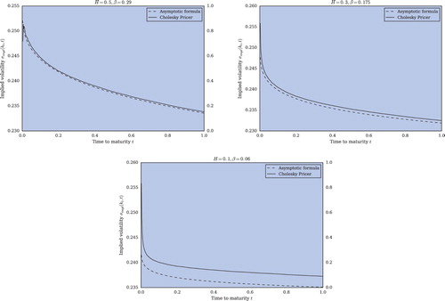
Numerical simulations³ confirm the theoretical results obtained in the last section. In particular – as can be seen in figure 1 – the asymptotic formula for the implied volatility (17(17) ${\sigma }_{\mathrm{impl}}(k_t,t)={\sigma }_0+\rho \frac{{\sigma }_0^{\mathrm{\prime }}}{{\sigma }_0}⟨K1,1⟩k{t}^{\beta }+\mathcal{O}\left({\phi }_{3,H,\beta ,\theta }\right(t\left)\right).$(17) ) captures very well the geometry of the term structure of implied volatility, with particularly good results for higher H and worsening results as $H\downarrow 0$. Quite surprisingly, despite being an asymptotic formula, it seems to be fairly accurate over a wide array of maturities extending up to a single year.

Figure 1. Illustration of the term structure of implied volatility of the Modified Rough Bergomi model in the Moderate deviations regime with time-varying log-strike $k_t=0.4t^{\beta }$. Depicted are the asymptotic formula (equation (17(17) ${\sigma }_{\mathrm{impl}}(k_t,t)={\sigma }_0+\rho \frac{{\sigma }_0^{\mathrm{\prime }}}{{\sigma }_0}⟨K1,1⟩k{t}^{\beta }+\mathcal{O}\left({\phi }_{3,H,\beta ,\theta }\right(t\left)\right).$(17) ), dashed line) and an estimate based on $N={10}^8$ samples of a MC Cholesky Option Pricer (solid line) with 500 time steps. Model parameters are given by spot vol ${\sigma }_0\approx 0.2557$, vvol $\eta =0.2928$ and correlation parameter $\rho =-0.7571$.

5. Proof of the energy expansion

Consider $\begin{array}{rl}\mathrm{d}X& =-\frac{1}{2}{\sigma }^2\left(Y\right)\mathrm{d}t+\sigma \left(Y\right)\mathrm{d}\left(\overline{\rho }\mathrm{d}W+\rho \mathrm{d}B\right),X_0=0\\ \mathrm{d}Y& =\mathrm{d}\hat{B},Y_0=0\end{array}$ where ${\hat{B}}_t={\int }_0^{t}K(t,s)\mathrm{d}{B}_s$ for a fixed Volterra kernel (recall (3(3) $\mathrm{d}{X}_t=-\frac{1}{2}{\sigma }^2\left({\hat{B}}_t\right)\mathrm{d}t+\sigma \left({\hat{B}}_t\right)\mathrm{d}\left(\overline{\rho }W+\rho B\right),X_0=0.$(3) ) in the previous section). We study the small noise problem $(X^{\epsilon },Y^{\epsilon })$ where $(W,B,\hat{B})$ is replaced by $(\epsilon W,\epsilon B,\hat{\epsilon }\hat{B})$. The following proposition roughly says that $\mathbb{P}\left(X_1^{\epsilon }\approx \frac{\epsilon }{\hat{\epsilon }}x\right)\approx \exp \left(-\frac{I\left(x\right)}{{\hat{\epsilon }}^2}\right).$

Proposition 5.1

Forde and Zhang 2017

Under suitable assumptions $($cf. Section 2), the rescaled process $\left(\right(\hat{\epsilon }/\epsilon )X_1^{\epsilon }:\epsilon \ge 0)$ satisfies an LDP $($with speed ${\hat{\epsilon }}^2)$ and rate function (24) $\begin{array}{rl}& I\left(x\right)=\underset{f\in H_0^1}{inf}\left[\frac{{\left(x-\rho G\left(f\right)\right)}^2}{2{\overline{\rho }}^{2}F\left(\hat{f}\right)}+\frac{1}{2}E\left(f\right)\right]\\ & \equiv \underset{f\in H_0^1}{inf}{\mathcal{I}}_x\left(f\right)\equiv {\mathcal{I}}_x\left(f^x\right),\end{array}$(24) where $\begin{array}{rl}G\left(f\right)& ={\int }_0^1\sigma \left(\left(K\dot{f}\right)\left(s\right)\right){\dot{f}}_s\mathrm{d}s\equiv ⟨\sigma \left(K\dot{f}\right),\dot{f}⟩\equiv ⟨\sigma \left(\hat{f}\right),\dot{f}⟩\\ F\left(f\right)& ={\int }_0^1\sigma {\left(\left(K\dot{f}\right)\left(s\right)\right)}^2\mathrm{d}s\equiv ⟨{\sigma }^2\left(K\dot{f}\right),1⟩\equiv ⟨{\sigma }^2\left(\hat{f}\right),1⟩\\ E\left(f\right)& ={\int }_0^1{\left|\dot{f}\left(s\right)\right|}^2\mathrm{d}s\equiv ⟨\dot{f},\dot{f}⟩\end{array}$

The rest of this section is devoted to analysis of the function I as defined in (24(24) $\begin{array}{rl}& I\left(x\right)=\underset{f\in H_0^1}{inf}\left[\frac{{\left(x-\rho G\left(f\right)\right)}^2}{2{\overline{\rho }}^{2}F\left(\hat{f}\right)}+\frac{1}{2}E\left(f\right)\right]\\ & \equiv \underset{f\in H_0^1}{inf}{\mathcal{I}}_x\left(f\right)\equiv {\mathcal{I}}_x\left(f^x\right),\end{array}$(24) ). First, we derive the first order optimality condition for the above minimization problem.

Proposition 5.2

First order optimality condition

For any $x\in \mathbb{R}$ we have at any local minimizer $f=f^x$ of the functional ${\mathcal{I}}_x$ in (24(24) $\begin{array}{rl}& I\left(x\right)=\underset{f\in H_0^1}{inf}\left[\frac{{\left(x-\rho G\left(f\right)\right)}^2}{2{\overline{\rho }}^{2}F\left(\hat{f}\right)}+\frac{1}{2}E\left(f\right)\right]\\ & \equiv \underset{f\in H_0^1}{inf}{\mathcal{I}}_x\left(f\right)\equiv {\mathcal{I}}_x\left(f^x\right),\end{array}$(24) ) that (25) $\begin{array}{rl}{f}_t^x& =\frac{\rho \left(x-\rho G\left(f^x\right)\right)\left\{⟨\sigma \left(K{\dot{f}}^x\right),1_{\left[0,t\right]}⟩+⟨{\sigma }^{\mathrm{\prime }}\left(K{\dot{f}}^x\right){\dot{f}}^x,K{1}_{\left[0,t\right]}⟩\right\}}{{\overline{\rho }}^{2}F\left(f^x\right)}\\ & +\frac{{\left(x-\rho G\left(f^x\right)\right)}^2}{{\overline{\rho }}^2{F}^2\left(f^x\right)}⟨\left(\sigma {\sigma }^{\mathrm{\prime }}\right)\left(K{\dot{f}}^x\right),K{1}_{\left[0,t\right]}⟩,\end{array}$(25) for all $t\in [0,1]$.

Proof.

We denote $a\approx b$ whenever $a=b+o\left(\delta \right)$ for a small parameter δ. We expand $\begin{array}{rl}E\left(f+\delta g\right)& \approx E\left(f\right)+2\delta ⟨\dot{f},\dot{g}⟩\\ F\left(f+\delta g\right)& \approx F\left(f\right)+\delta ⟨{\left({\sigma }^2\right)}^{\mathrm{\prime }}\left(K\dot{f}\right),K\dot{g}⟩\\ G\left(f+\delta g\right)& \approx G\left(f\right)+\delta \left\{⟨\sigma \left(K\dot{f}\right),\dot{g}⟩+⟨{\sigma }^{\mathrm{\prime }}\left(K\dot{f}\right)\dot{f},K\dot{g}⟩\right\}\end{array}$ If $f=f^x$ is a minimizer then $\delta \mapsto {\mathcal{I}}_x(f+\delta g)$ has a minimum at $\delta =0$ for all g. We expand $\begin{array}{rl}& {\mathcal{I}}_x\left(f+\delta g\right)=\frac{{\left(x-\rho G\left(f+\delta g\right)\right)}^2}{2{\overline{\rho }}^{2}F\left(f+\delta g\right)}+\frac{1}{2}E(f+\delta g)\\ & \approx \frac{{\left(x-\rho G\left(f\right)-\delta \rho \left\{⟨\sigma \left(K\dot{f}\right),\dot{g}⟩+⟨{\sigma }^{\mathrm{\prime }}\left(K\dot{f}\right)\dot{f},K\dot{g}⟩\right\}\right)}^2}{2{\overline{\rho }}^2\left[F\left(f\right)+\delta ⟨{\left({\sigma }^2\right)}^{\mathrm{\prime }}\left(K\dot{f}\right),K\dot{g}⟩\right]}\\ & +\frac{1}{2}E\left(f\right)+\delta ⟨\dot{f},\dot{g}⟩\\ & \approx \frac{\begin{array}{c}{\left(x-\rho G\left(f\right)\right)}^2-\delta 2\rho \left(x-\rho G\left(f\right)\right)\\ \left\{⟨\sigma \left(K\dot{f}\right),\dot{g}⟩+⟨{\sigma }^{\mathrm{\prime }}\left(K\dot{f}\right)\dot{f},K\dot{g}⟩\right\}\end{array}}{2{\overline{\rho }}^{2}F\left(f\right)\left[1+\frac{\delta }{F\left(f\right)}⟨{\left({\sigma }^2\right)}^{\mathrm{\prime }}\left(K\dot{f}\right),K\dot{g}⟩\right]}\\ & +\frac{1}{2}E\left(f\right)+\delta ⟨\dot{f},\dot{g}⟩\\ & \approx \frac{\begin{array}{c}{\left(x-\rho G\left(f\right)\right)}^2-\delta 2\rho \left(x-\rho G\left(f\right)\right)\\ \left\{⟨\sigma \left(K\dot{f}\right),\dot{g}⟩+⟨{\sigma }^{\mathrm{\prime }}\left(K\dot{f}\right)\dot{f},K\dot{g}⟩\right\}\end{array}}{2{\overline{\rho }}^{2}F\left(f\right)}\\ & -\frac{{\left(x-\rho G\left(f\right)\right)}^2}{2{\overline{\rho }}^{2}F\left(f\right)}\frac{\delta }{F\left(f\right)}⟨{\left({\sigma }^2\right)}^{\mathrm{\prime }}\left(K\dot{f}\right),K\dot{g}⟩+\frac{1}{2}E\left(f\right)\\ & +\delta ⟨\dot{f},\dot{g}⟩.\end{array}$ As a consequence, we must have, for $f=f^x$ and every $\dot{g}\in L^2[0,1]$ $\begin{array}{rl}0& =\frac{\mathrm{d}}{\mathrm{d}\delta }{\left\{{\mathcal{I}}_x\left(f+\delta g\right)\right\}}_{\delta =0}\\ & =-\frac{\rho \left(x-\rho G\left(f\right)\right)\left\{⟨\sigma \left(K\dot{f}\right),\dot{g}⟩+⟨{\sigma }^{\mathrm{\prime }}\left(K\dot{f}\right)\dot{f},K\dot{g}⟩\right\}}{{\overline{\rho }}^{2}F\left(f\right)}\\ & -\frac{{\left(x-\rho G\left(f\right)\right)}^2}{{\overline{\rho }}^2{F}^2\left(f\right)}⟨\left(\sigma {\sigma }^{\mathrm{\prime }}\right)\left(K\dot{f}\right),K\dot{g}⟩+⟨\dot{f},\dot{g}⟩.\end{array}$ Recall $f_0^x=0$, any x. We now test with $\dot{g}=1_{[0,t]}$ for a fixed $t\in [0,1]$ and obtain $\begin{array}{rl}{f}_t^x& =\frac{\rho \left(x-\rho G\left(f^x\right)\right)\left\{⟨\sigma \left(K{\dot{f}}^x\right),1_{\left[0,t\right]}⟩+⟨{\sigma }^{\mathrm{\prime }}\left(K{\dot{f}}^x\right){\dot{f}}^x,K{\mathbf{1}}_{\left[0,t\right]}⟩\right\}}{{\overline{\rho }}^{2}F\left(f^x\right)}\\ & +\frac{{\left(x-\rho G\left(f^x\right)\right)}^2}{{\overline{\rho }}^2{F}^2\left(f^x\right)}⟨\left(\sigma {\sigma }^{\mathrm{\prime }}\right)\left(K{\dot{f}}^x\right),K{\mathbf{1}}_{\left[0,t\right]}⟩.\end{array}$

5.1. Smoothness of the energy

Having formally identified the first order condition for minimality in (24(24) $\begin{array}{rl}& I\left(x\right)=\underset{f\in H_0^1}{inf}\left[\frac{{\left(x-\rho G\left(f\right)\right)}^2}{2{\overline{\rho }}^{2}F\left(\hat{f}\right)}+\frac{1}{2}E\left(f\right)\right]\\ & \equiv \underset{f\in H_0^1}{inf}{\mathcal{I}}_x\left(f\right)\equiv {\mathcal{I}}_x\left(f^x\right),\end{array}$(24) ), we will now show that the energy $x\mapsto I\left(x\right)$ is a smooth function. More precisely, we will use the implicit function theorem to show that the minimizing configuration $f^x$ is a smooth function in x (locally at x=0). As ${\mathcal{I}}_x$ is a smooth function, too, this will imply smoothness of $x\mapsto {\mathcal{I}}_x\left(f^x\right)=I\left(x\right)$, at least in a neighborhood of 0.

As the Cameron-Martin space $\mathcal{H}$ of the process $\hat{B}$ continuously embeds into $C\left(\right[0,1\left]\right)$, K maps $H_0^1$ continuously into $C\left(\right[0,1\left]\right)$, i.e. there is a constant C>0 such that for any $f\in H_0^1$ we have (26) ${∥K\dot{f}∥}_{\mathrm{\infty }}\le C{∥f∥}_{H_0^1}.$(26) This result will follow from

Lemma 5.3

Let $(V_t:0\le t\le 1)$ be a continuous, centred Gaussian process and $\mathcal{H}$ its Cameron-Martin space. Then we have the continuous embedding $\mathcal{H}\hookrightarrow C[0,1]$. That is, for some constant C, ${∥h∥}_{\mathrm{\infty }}\le C{∥h∥}_{\mathcal{H}}.$

Proof.

By a fundamental result of Fernique, applied to the law of V as Gaussian measure on the Banach space $\left(C\right[0,1],\parallel \cdot {\parallel }_{\mathrm{\infty }})$, the random variable $\parallel V{\parallel }_{\mathrm{\infty }}$ has Gaussian integrability. In particular, ${\sigma }^2:=\mathbb{E}\mathbb{(}{∥V∥}_{\mathrm{\infty }}^2)<\mathrm{\infty },$ On the other hand, a generic element $h\in \mathcal{H}$ can be written as $h_t=E\left[V_{t}Z\right]$ where Z is a centred Gaussian random variable with variance $\parallel h{\parallel }_{\mathcal{H}}^2$, see, e.g. Friz and Hairer (2014, page 150). By Cauchy–Schwarz, $\left|h_t\right|\le E{\left[\left|V_t\right|\right]}^{1/2}{∥h∥}_{\mathcal{H}}\le \sigma {∥h∥}_{\mathcal{H}}$ and conclude by taking the $sup$ over on the l.h.s. over $t\in [0,1]$.

Remark 5.4

Assume V is of Volterra form, i.e. $V_t={\int }_0^{t}K(t,s)\mathrm{d}{B}_s$. Then it can be shown (see Decreusefond 2005, Section 3) that $\mathcal{H}$ is the image of $L^2$ under the map $K:\dot{f}\mapsto \hat{f}:=\left(t\mapsto {\int }_0^{t}K\left(t,s\right){\dot{f}}_s\mathrm{d}s\right)$ and $\parallel K\dot{f}{\parallel }_{\mathcal{H}}=\parallel \dot{\phantom{a}}f{\parallel }_{L^2}$. In particular then, applying the above with $h=K\dot{f}\in \mathcal{H}$, gives ${∥K\dot{f}∥}_{\mathrm{\infty }}\le C{∥K\dot{f}∥}_{\mathcal{H}}=C{∥\dot{f}∥}_{L^2}=C{∥f∥}_{H_0^1}.$

5.1.1. The uncorrelated case

We start with the case $\rho =0$ as the formulas are much simpler in this case.

By Proposition 5.2, any local optimizer $f=f^x$ of the functional ${\mathcal{I}}_x:H_0^1\to \mathbb{R}$ in the uncorrelated case $\rho =0$ satisfies for any $t\in [0,1]$ $f_t=\frac{x^2}{F^2\left(f\right)}⟨\left(\sigma {\sigma }^{\mathrm{\prime }}\right)\left(K\dot{f}\right),K{\mathbf{1}}_{[0,t]}⟩.$ We define a map $H:H_0^1\times \mathbb{R}\to H_0^1$ by (27) $H(f,x)\left(t\right):=f_t-\frac{x^2}{F^2\left(f\right)}⟨\left(\sigma {\sigma }^{\mathrm{\prime }}\right)\left(K\dot{f}\right),K{\mathbf{1}}_{[0,t]}⟩.$(27) Hence, for given $x\in \mathbb{R}$, any local optimizer f must solve $H(f,x)=0$. As one particular solution is given by the pair $(0,0)$, we are in the realm of the implicit function theorem. We need to prove that

• $(f,x)\mapsto H(f,x)$ is locally smooth (in the sense of Fréchet);

• $DH(f,x):=\left(\mathrm{\partial }/\mathrm{\partial }f\right)H(f,x)$ is invertible in $(0,0)$.

Note that invertibility should hold for x small enough, as $DH(f,x)={\mathrm{id}}_{H_0^1}-x^{2}R$ for some R, which is invertible as long as R has a bounded norm for sufficiently small x.

Remark 5.5

The method of proof in this section is purely local in $H_0^1$. Hence, we only really need smoothness of σ locally around 0. Note, however, that stochastic Taylor expansions used in Section 6 will actually require global smoothness of σ.

Lemma 5.6

The functions $F:H_0^1\to \mathbb{R}$ and $R_1:H_0^1\to C\left(\right[0,1\left]\right)$ defined by $R_1\left(f\right)\left(t\right):=⟨\left(\sigma {\sigma }^{\mathrm{\prime }}\right)\left(K\dot{f}\right),K{\mathbf{1}}_{[0,t]}⟩,t\in [0,1],$ are smooth in the sense of Fréchet.

Proof.

For $N\ge 1$ we note that the Gateaux derivative of F satisfies $D^{N}F\left(f\right)\cdot \left(g_1,\dots ,g_N\right)={\int }_0^1\frac{{\mathrm{d}}^N}{\mathrm{d}{x}^N}{\sigma }^2\left(K\dot{f}\right)K{\dot{g}}_1\cdots K{\dot{g}}_N\mathrm{d}s.$ By Lemma 5.3, we can bound $\begin{array}{rl}∣D^{N}F\left(f\right)\cdot \left(g_1,\dots ,g_N\right)∣& \le \mathrm{const}{\int }_0^1∣K\dot{g_1}\left(s\right)∣\cdots ∣K\dot{g_N}\left(s\right)∣\mathrm{d}s\\ & \le \mathrm{const}{∥K{\dot{g}}_1∥}_{\mathrm{\infty }}\cdots {∥K{\dot{g}}_N∥}_{\mathrm{\infty }}\\ & \le \mathrm{const}{C}^N{∥g_1∥}_{H_0^1}\cdots {∥g_N∥}_{H_0^1},\end{array}$ for $\mathrm{const}={∥\left({\mathrm{d}}^n/\mathrm{d}{x}^n\right){\sigma }^2∥}_{\mathrm{\infty }}$.⁴ Thus, $D^{N}F\left(f\right)$ is a multi-linear form on $H_0^1$ with operator norm $∥D^{N}F\left(f\right)∥\le {∥\left({\mathrm{d}}^n/\mathrm{d}{x}^n\right){\sigma }^2∥}_{\mathrm{\infty }}{C}^N$ independent of f. As $f\mapsto D^{N}F\left(f\right)$ is continuous, we conclude that $D^{N}F\left(f\right)$ as given above is, in fact, a Fréchet derivative.

Let us next consider the functional $R_1$. Note that $\left(D^N{R}_1\left(f\right)\cdot (g_1,\dots ,g_N)\right)\left(t\right)=⟨{\mathfrak{s}}_N\left(K\dot{f}\right)K{\dot{g}}_1\cdots K{\dot{g}}_N,K{\mathbf{1}}_{[0,t]}⟩$ for ${\mathfrak{s}}_N\left(x\right):=\left({\mathrm{d}}^N/\mathrm{d}{x}^N\right)\sigma \left(x\right){\sigma }^{\mathrm{\prime }}\left(x\right)$. Hence, Assumption 2.5 implies that $\begin{array}{rl}& {∥D^N{R}_1\left(f\right)\cdot (g_1,\dots ,g_N)∥}_{H_0^1}^2\\ & ={\int }_0^1{\left({\int }_t^1{\mathfrak{s}}_N\left(\left(K\dot{f}\right)\left(s\right)\right)\prod _{i=1}^N\left(K{\dot{g}}_i\right)\left(s\right)K(s,t)\mathrm{d}s\right)}^2\mathrm{d}t\\ & \le {∥{\mathfrak{s}}_N∥}_{\mathrm{\infty }}^2\prod _{i=1}^N{∥K{\dot{g}}_i∥}_{\mathrm{\infty }}^2{\int }_0^1{\int }_t^{1}K(s,t{)}^2\mathrm{d}s\mathrm{d}t\\ & \le {∥{\mathfrak{s}}_N∥}_{\mathrm{\infty }}^2{C}^{2N}\prod _{i=1}^N{∥g_i∥}_{H_0^1}^2{\int }_0^1{\int }_0^{s}K(s,t{)}^2\mathrm{d}t\mathrm{d}s\\ & \le {∥{\mathfrak{s}}_N∥}_{\mathrm{\infty }}^2{C}^{2N}{\int }_0^1{\int }_0^{s}K(s,t{)}^2\mathrm{d}t\mathrm{d}s\prod _{i=1}^N{∥g_i∥}_{H_0^1}^2.\end{array}$ We see that the multi-linear map $D^N{R}_1\left(f\right)$ has operator norm bounded by $∥D^N{R}_1\left(f\right)∥\le {∥{\mathfrak{s}}_N∥}_{\mathrm{\infty }}{C}^N\sqrt{{\int }_0^1{\int }_0^{s}K(s,t{)}^2\mathrm{d}t\mathrm{d}s},$ independent of f. From continuity of $f\mapsto D^N{R}_1\left(f\right)$, it follows that $D^N{R}_1\left(f\right)$ is the N'th Fréchet derivative.

Theorem 5.7

Zero correlation

Assuming $\rho =0,$ the energy $I\left(x\right)$ $($as defined in (24(24) $\begin{array}{rl}& I\left(x\right)=\underset{f\in H_0^1}{inf}\left[\frac{{\left(x-\rho G\left(f\right)\right)}^2}{2{\overline{\rho }}^{2}F\left(\hat{f}\right)}+\frac{1}{2}E\left(f\right)\right]\\ & \equiv \underset{f\in H_0^1}{inf}{\mathcal{I}}_x\left(f\right)\equiv {\mathcal{I}}_x\left(f^x\right),\end{array}$(24) )) is smooth in a neighborhood of x=0.

Proof.

By construction, we have $DH(f,x)={\mathrm{id}}_{H_0^1}-x^{2}A\left(f\right)$ for $A:H_0^1\to \mathcal{L}(H_0^1,H_0^1)$ defined by $A\left(f\right):=R_1\left(f\right)\otimes D{F}^{-2}\left(f\right)+F^{-2}\left(f\right)D{R}_1\left(f\right).$ Here, $\left(R_1\left(f\right)\otimes D{F}^{-2}\left(f\right)\right)\cdot g=\underset{\in \mathbb{R}}{\underbrace{\left(D{F}^{-2}\right(f)\cdot g)}}\underset{\in H_0^1}{\underbrace{R_1\left(f\right)}}.$ As verified above, H is smooth in the sense of Fréchet. Trivially, $DH(0,0)={\mathrm{id}}_{H_0^1}$ is invertible and $H(0,0)=0$. Therefore, the implicit function theorem implies that there are open neighborhoods U and V of $0\in H_0^1$ and $0\in \mathbb{R}$, respectively, and a smooth map $x\mapsto f^x$ from V to U such that $H(f^x,x)\equiv 0$ and $f^x$ is unique in U with this property.

For the energy, we prove that $I\left(x\right)={\mathcal{I}}_x\left(f^x\right)$ in a neighborhood of x=0. First of all, we show that a minimizer exists. If not, there is a function $g\in H_0^1$ with ${\mathcal{I}}_x\left(g\right)<{\mathcal{I}}_x\left(f^x\right)$. For small enough x such a g must be inside a ball with radius ε around $0\in H_0^1$, as ${\mathcal{I}}_x\left(g\right)\ge \frac{1}{2}{∥g∥}_{H_0^1}^2$ and $\underset{x\to 0}{lim}{\mathcal{I}}_x\left(f^x\right)=0$. Then note that for any $g\in H_0^1$ $D^2{\mathcal{I}}_0\left(0\right)\cdot (g,g)={∥g∥}_{H_0^1}^2>0,$ where $D^2{\mathcal{I}}_x\left(f\right)$ denotes the second derivative of $f\mapsto {\mathcal{I}}_x\left(f\right)$. By continuity, $D^2{\mathcal{I}}_x\left(f\right)$ stays positive definite for $(x,f)$ in a neighborhood of $(0,0)$. As noted, for x small enough, both g and $f^x$ (and the line connecting them) lie in this neighborhood. For $h:=g-f^x$, this implies $\begin{array}{rl}& {\mathcal{I}}_x\left(g\right)-{\mathcal{I}}_x\left(f^x\right)=D{\mathcal{I}}_x\left(f_x\right)\cdot h\\ & +{\int }_0^1{D}^2{\mathcal{I}}_x(f^x+th)\cdot (h,h)\mathrm{d}t>0,\end{array}$ since $D{\mathcal{I}}_x\left(f_x\right)\cdot h=0$ and $D^2{\mathcal{I}}_x(f^x+tsh)\cdot (h,h)>0$. This contradicts the assumption that ${\mathcal{I}}_x\left(g\right)<{\mathcal{I}}_x\left(f^x\right)$, and we conclude that $f^x$ is, indeed, a minimizer of ${\mathcal{I}}_x$, implying that $I\left(x\right)={\mathcal{I}}_x\left(f^x\right)$ locally.

Finally, as $x\mapsto f^x$ is smooth and $(f,x)\mapsto {\mathcal{I}}_x\left(f\right)=x^2/2F\left(f\right)+\frac{1}{2}{∥f∥}_{H_0^1}^2$ is smooth, we see that $x\mapsto I\left(x\right)={\mathcal{I}}_x\left(f^x\right)$ is smooth in a neighborhood of 0. (Note that this arguments relies on $\sigma \left(0\right)\ne 0$, implying that $F\left(f\right)\ne 0$ for f in a neighborhood to 0.)

Remark 5.8

Classical counter-examples in the context of the direct method of calculus of variations show that the step of verifying the existence of a minimizer should not be taken too lightly. For instance, the functional $J\left(u\right):={\int }_0^1\left[\left(u^{\mathrm{\prime }}\right(s{)}^2-1{)}^2+u(s{)}^2\right]\mathrm{d}s$ does not have a minimizer in $H_0^1$, but J can be made arbitrarily close to 0 by choosing piecewise-linear functions u with slope $∣u^{\mathrm{\prime }}∣=1$ oscillating around 0. We refer to any text book on calculus of variations. In the situation above, local ‘convexity’ in the sense of a positive definite second derivative prevents this phenomenon. An alternative method of proof for the existence of a minimizer is to show that J is (lower semi-) continuous in the weak sense.

5.1.2. The general case

In the general case (cf. Proposition 5.2), we define the function $H:H_0^1\times \mathbb{R}\to H_0^1$ by (28) $\begin{array}{rl}& H(f,x)\left(t\right)\\ & :=f_t-\frac{\begin{array}{c}\rho \left(x-\rho G\left(f\right)\right)\\ \left\{⟨\sigma \left(K\dot{f}\right),{\mathbf{1}}_{[0,t]}⟩+⟨{\sigma }^{\mathrm{\prime }}\left(K\dot{f}\right)\dot{f},K{\mathbf{1}}_{[0,t]}⟩\right\}\end{array}}{{\overline{\rho }}^{2}F\left(f\right)}\\ & +\frac{{\left(x-\rho G\left(f\right)\right)}^2}{{\overline{\rho }}^2{F}^2\left(f\right)}⟨\left(\sigma {\sigma }^{\mathrm{\prime }}\right)\left(K\dot{f}\right),K{\mathbf{1}}_{[0,t]}⟩\\ & =f_t-\frac{\rho \left(x-\rho G\left(f\right)\right)}{{\overline{\rho }}^{2}F\left(f\right)}\left(R_2\left(f\right)\left(t\right)+R_3\left(f\right)\left(t\right)\right)\\ & +\frac{{\left(x-\rho G\left(f\right)\right)}^2}{{\overline{\rho }}^{2}F(f{)}^2}{R}_1\left(f\right)\left(t\right),\end{array}$(28) where $R_2,R_3:H_0^1\to H_0^1$ are defined by (29) $\begin{array}{rl}{R}_2\left(f\right)\left(t\right)& :=⟨\sigma \left(K\dot{f}\right),{\mathbf{1}}_{[0,t]}⟩,\end{array}$(29) (30) $\begin{array}{rl}{R}_3\left(f\right)\left(t\right)& :=⟨{\sigma }^{\mathrm{\prime }}\left(K\dot{f}\right)\dot{f},K{\mathbf{1}}_{[0,t]}⟩,\end{array}$(30) $t\in [0,1]$.

One easily checks that G, $R_2$, $R_3$ are smooth in the Fréchet sense.

Lemma 5.9

The functions $G:H_0^1\to \mathbb{R},$ $R_2:H_0^1\to H_0^1$ and $R_3:H_0^1\to H_0^1$ are smooth in Fréchet sense.

Proof.

The proof of smoothness is clear. We report the actual derivatives. For G we get $\begin{array}{rl}{D}^{N}G\left(f\right)& \cdot \left(g_1,\dots ,g_N\right)=⟨{\sigma }^{\left(N\right)}\left(K\dot{f}\right)\dot{f},\prod _{i=1}^{N}K{\dot{g}}_i⟩\\ & +\sum _{k=1}^N⟨{\sigma }^{(N-1)}\left(K\dot{f}\right),{\dot{g}}_k\prod _{i\ne k}K{\dot{g}}_i⟩.\end{array}$ For $R_2$ and, respectively, $R_3$, we obtain $\begin{array}{rl}& \left(D^N{R}_2\left(f\right)\cdot (g_1,\dots ,g_N)\right)\left(t\right)\\ & ={\int }_0^t{\sigma }^{\left(N\right)}\left(\left(K\dot{f}\right)\left(s\right)\right)\prod _{i=1}^N\left(K{\dot{g}}_i\right)\left(s\right)\mathrm{d}s,\end{array}$ and $\begin{array}{rl}& \left(D^N{R}_3\left(f\right)\cdot (g_1,\dots ,g_N)\right)\left(t\right)\\ & =⟨{\sigma }^{(N+1)}\left(K\dot{f}\right)\dot{f}K{\mathbf{1}}_{[0,t]},\prod _{i=1}^{N}K{\dot{g}}_i⟩\\ & +\sum _{k=1}^N⟨{\sigma }^{\left(N\right)}\left(K\dot{f}\right)K{\mathbf{1}}_{[0,t]},{\dot{g}}_k\prod _{i\ne k}K{\dot{g}}_i⟩.\end{array}$

Theorem 5.10

Let σ be smooth with $\sigma \left(0\right)\ne 0$. Then the energy $I\left(x\right)$ as defined in (24(24) $\begin{array}{rl}& I\left(x\right)=\underset{f\in H_0^1}{inf}\left[\frac{{\left(x-\rho G\left(f\right)\right)}^2}{2{\overline{\rho }}^{2}F\left(\hat{f}\right)}+\frac{1}{2}E\left(f\right)\right]\\ & \equiv \underset{f\in H_0^1}{inf}{\mathcal{I}}_x\left(f\right)\equiv {\mathcal{I}}_x\left(f^x\right),\end{array}$(24) ) is smooth in a neighborhood of x=0.

Proof.

The proof is similar to the proof of Theorem 5.7. In fact, the only difference is in establishing invertibility of $DH(0,0)$ and the existence of a minimizer.

Note that (28(28) $\begin{array}{rl}& H(f,x)\left(t\right)\\ & :=f_t-\frac{\begin{array}{c}\rho \left(x-\rho G\left(f\right)\right)\\ \left\{⟨\sigma \left(K\dot{f}\right),{\mathbf{1}}_{[0,t]}⟩+⟨{\sigma }^{\mathrm{\prime }}\left(K\dot{f}\right)\dot{f},K{\mathbf{1}}_{[0,t]}⟩\right\}\end{array}}{{\overline{\rho }}^{2}F\left(f\right)}\\ & +\frac{{\left(x-\rho G\left(f\right)\right)}^2}{{\overline{\rho }}^2{F}^2\left(f\right)}⟨\left(\sigma {\sigma }^{\mathrm{\prime }}\right)\left(K\dot{f}\right),K{\mathbf{1}}_{[0,t]}⟩\\ & =f_t-\frac{\rho \left(x-\rho G\left(f\right)\right)}{{\overline{\rho }}^{2}F\left(f\right)}\left(R_2\left(f\right)\left(t\right)+R_3\left(f\right)\left(t\right)\right)\\ & +\frac{{\left(x-\rho G\left(f\right)\right)}^2}{{\overline{\rho }}^{2}F(f{)}^2}{R}_1\left(f\right)\left(t\right),\end{array}$(28) ) contains three terms. The derivative of the first term ($f\mapsto f$) is always equal to ${\mathrm{id}}_{H_0^1}$. For the second term, we note that ${\left.\left(x-\rho G\left(f\right)\right)\right|}_{x=0,f=0}=0.$ Hence, the only non-vanishing contribution to the derivative of the second term evaluated in direction $g\in H_0^1$ at x=0, f=0 and $t\in [0,1]$ is $\begin{array}{rl}& \frac{{\rho }^{2}DG\left(0\right)\cdot g}{{\overline{\rho }}^{2}F\left(0\right)}\left(R_2\right(0)+R_3(0\left)\right)=\frac{{\rho }^2{\sigma }_{0}g\left(1\right)}{{\overline{\rho }}^2{\sigma }_0^2}\left({\sigma }_{0}t+0\right)\\ & =\frac{{\rho }^2}{{\overline{\rho }}^2}g\left(1\right)t.\end{array}$ For the same reason, the derivative of the third term at $(f,x)=(0,0)$ vanishes entirely. Hence, $\left(DH\right(0,0)\cdot g)\left(t\right)=g\left(t\right)+\frac{{\rho }^2}{{\overline{\rho }}^2}g\left(1\right)t.$ It is easy to see that $g\mapsto DH(0,0)\cdot g$ is invertible. Indeed, let us construct the pre-image $g=DH(0,0{)}^{-1}\cdot h$ of some $h\in H_0^1$. At t=1 we have $\frac{{\overline{\rho }}^2+{\rho }^2}{{\overline{\rho }}^2}g\left(1\right)=h\left(1\right),$ implying $g\left(1\right)={\overline{\rho }}^{2}h\left(1\right)$. For $0\le t<1$, we then get $\begin{array}{rl}& g\left(t\right)+\frac{{\rho }^2}{{\overline{\rho }}^2}g\left(1\right)t=g\left(t\right)+\frac{{\rho }^2}{{\overline{\rho }}^2}{\overline{\rho }}^{2}h\left(1\right)t\\ & =g\left(t\right)+{\rho }^{2}h\left(1\right)t=h\left(t\right),\end{array}$ or $g\left(t\right)=h\left(t\right)-{\rho }^{2}h\left(1\right)t$.

For existence of the minimizer, note that $D^2{J}_0\left(0\right)\cdot (g,g)=\frac{{\rho }^2}{{\overline{\rho }}^2}g(1{)}^2+{∥g∥}_{H_0^1}^2,$ which is again positive definite.

Remark 5.11

Though only formulated in terms of ‘smoothness’, it is easy to show that $\sigma \in C^k$ implies that $I\in C^{k-1}$ (locally at 0).

5.2. Energy expansion

Having established smoothness of the energy I as well as of the minimizing configuration $x\mapsto f^x$ locally around x=0, we can proceed with computing the Taylor expansion of $f^x$ around x=0. We will once more rely on the first order optimality condition given in Proposition 5.2. Plugging the Taylor expansion of $f^x$ into ${\mathcal{I}}_x$ will then give us the local Taylor expansion of $I\left(x\right)$.

5.2.1. Expansion of the minimizing configuration

Theorem 5.12

We have $\begin{array}{rl}{f}_t^x& ={\alpha }_{t}x+{\beta }_t\frac{x^2}{2}+\mathcal{O}\left(x^3\right),\\ {\alpha }_t& =\frac{\rho }{{\sigma }_0}t,\\ {\beta }_t& =2\frac{{\sigma }_0^{\mathrm{\prime }}}{{\sigma }_0^3}\left[{\rho }^2⟨K1,{\mathbf{1}}_{[0,t]}⟩+⟨K{\mathbf{1}}_{[0,t]},1⟩-3{\rho }^{2}t⟨K1,1⟩\right].\end{array}$

Remark 5.13

Non-Markovian transversality

In the RL-fBM case, $K(t,s)=\sqrt{2H}|t-s{|}^{\gamma }$ with $\gamma =H-1/2$ one computes $⟨1,K{1}_{\left[0,t\right]}⟩=\frac{1}{\left(1+\gamma \right)\left(2+\gamma \right)}\left\{1-{\left(1-t\right)}^{2+\gamma }\right\}\in C^1\left[0,1\right].$ Interestingly, the transversality condition known from the Markovian setting ($q_1=0$, which readily translates to ${\dot{f}}_1^x=0$ there) remains valid here (for $\rho =0$), at least to order $x^2$, in the sense that ${\dot{f}}_t^x\approx {\beta }_t\frac{x^2}{2}=\left(\mathrm{const}\right){\left(1-t\right)}^{1+\gamma }{|}_{t=1}=0$

Proof of Theorem 5.12

First order expansion:

Up to the order needed in order to get the first order term, we have $\begin{array}{rl}{f}_t^x& ={\alpha }_{t}x+\mathcal{O}\left(x^2\right),\\ {\dot{f_t}}^x& =\dot{{\alpha }_t}x+\mathcal{O}\left(x^2\right),\\ \sigma \left(K{\dot{f}}^x\right)& ={\sigma }_0+{\sigma }_0^{\prime }K\dot{\alpha }x+\mathcal{O}\left(x^2\right),\\ {\sigma }^{\prime }\left(K{\dot{f}}^x\right)& ={\sigma }_0^{\prime }+{\sigma }_0^{″}K\dot{\alpha }x+\mathcal{O}\left(x^2\right),\\ F\left(f^x\right)& =⟨{\sigma }^2\left(K{\dot{f}}^x\right),1⟩\\ & ={\sigma }_0^2+\mathcal{O}\left(x\right),\\ G\left(f^x\right)& =⟨\sigma \left(K{\dot{f}}^x\right),{\dot{f}}^x⟩\\ & =⟨{\sigma }_0,\dot{\alpha }⟩x+\mathcal{O}\left(x^2\right).\end{array}$ Therefore, $\begin{array}{rl}⟨\sigma \left(K{\dot{f}}^x\right),{\mathbf{1}}_{[0,t]}⟩& ={\sigma }_{0}t+\mathcal{O}\left(x\right),\\ ⟨{\sigma }^{\prime }\left(K{\dot{f}}^x\right){\dot{f}}^x,K{\mathbf{1}}_{[0,t]}⟩& =\mathcal{O}\left(x\right),\\ ⟨\sigma {\sigma }^{\prime }\left(K{\dot{f}}^x\right),K{\mathbf{1}}_{[0,t]}⟩& =\mathcal{O}\left(1\right),\\ x-\rho G\left(f^x\right)& =(1-\rho {\sigma }_0{\alpha }_1)x+\mathcal{O}\left(x^2\right),\\ (x-\rho G(f^x){)}^2& =\mathcal{O}\left(x^2\right).\end{array}$ This yields for the first order term in (25(25) $\begin{array}{rl}{f}_t^x& =\frac{\rho \left(x-\rho G\left(f^x\right)\right)\left\{⟨\sigma \left(K{\dot{f}}^x\right),1_{\left[0,t\right]}⟩+⟨{\sigma }^{\mathrm{\prime }}\left(K{\dot{f}}^x\right){\dot{f}}^x,K{1}_{\left[0,t\right]}⟩\right\}}{{\overline{\rho }}^{2}F\left(f^x\right)}\\ & +\frac{{\left(x-\rho G\left(f^x\right)\right)}^2}{{\overline{\rho }}^2{F}^2\left(f^x\right)}⟨\left(\sigma {\sigma }^{\mathrm{\prime }}\right)\left(K{\dot{f}}^x\right),K{1}_{\left[0,t\right]}⟩,\end{array}$(25) ) ${\alpha }_t=\frac{\rho (1-\rho {\sigma }_0{\alpha }_1)}{{\overline{\rho }}^2{\sigma }_0}t.$ Setting t=1, we get ${\alpha }_1=\frac{\rho }{{\overline{\rho }}^2{\sigma }_0}-\frac{{\rho }^2}{{\overline{\rho }}^2}{\alpha }_1,$ which is solved by ${\alpha }_1=\rho /{\sigma }_0$. Inserting this term back into the equation for ${\alpha }_t$, we get (31) ${\alpha }_t=\frac{\rho }{{\sigma }_0}t.$(31)

Second order expansion:

Using (31(31) ${\alpha }_t=\frac{\rho }{{\sigma }_0}t.$(31) ) and the ansatz $f_t^x={\alpha }_{t}x+\frac{1}{2}{\beta }_t{x}^2+\mathcal{O}\left(x^3\right)$, we re-compute the relevant terms appearing in the (25(25) $\begin{array}{rl}{f}_t^x& =\frac{\rho \left(x-\rho G\left(f^x\right)\right)\left\{⟨\sigma \left(K{\dot{f}}^x\right),1_{\left[0,t\right]}⟩+⟨{\sigma }^{\mathrm{\prime }}\left(K{\dot{f}}^x\right){\dot{f}}^x,K{1}_{\left[0,t\right]}⟩\right\}}{{\overline{\rho }}^{2}F\left(f^x\right)}\\ & +\frac{{\left(x-\rho G\left(f^x\right)\right)}^2}{{\overline{\rho }}^2{F}^2\left(f^x\right)}⟨\left(\sigma {\sigma }^{\mathrm{\prime }}\right)\left(K{\dot{f}}^x\right),K{1}_{\left[0,t\right]}⟩,\end{array}$(25) ). We have $\sigma \left(K{\dot{f}}^x\right(s\left)\right)={\sigma }_0+{\sigma }_0^{\mathrm{\prime }}\frac{\rho }{{\sigma }_0}\left(K1\right)\left(s\right)x+\mathcal{O}\left(x^2\right)$ and analogously for σ replaced by ${\sigma }^{\mathrm{\prime }}$, $\sigma {\sigma }^{\mathrm{\prime }}$. This implies $\begin{array}{rl}& ⟨\sigma \left(K{\dot{f}}^x\right),{\mathbf{1}}_{[0,t]}⟩={\sigma }_{0}t+{\sigma }_0^{\mathrm{\prime }}\frac{\rho }{{\sigma }_0}⟨K1,{\mathbf{1}}_{[0,t]}⟩x+\mathcal{O}\left(x^2\right),\\ & ⟨{\sigma }^{\mathrm{\prime }}\left(K{\dot{f}}^x\right){\dot{f}}^x,K{\mathbf{1}}_{[0,t]}⟩=\rho \frac{{\sigma }^{\mathrm{\prime }}}{{\sigma }_0}⟨K{\mathbf{1}}_{[0,t]},1⟩x+\mathcal{O}\left(x^2\right),\\ & ⟨\sigma {\sigma }^{\mathrm{\prime }}\left(K{\dot{f}}^x\right),K{\mathbf{1}}_{[0,t]}⟩={\sigma }_0{\sigma }_0^{\mathrm{\prime }}⟨K{\mathbf{1}}_{[0,t]},1⟩+\mathcal{O}\left(x\right).\end{array}$ Using the notation introduced earlier, we have $\begin{array}{rl}& F\left(f^x\right)={\sigma }_0^2+2{\sigma }_0^{\mathrm{\prime }}\rho ⟨K1,1⟩x+\mathcal{O}\left(x^2\right),\\ & G\left(f^x\right)=\rho x+\left(\frac{1}{2}{\sigma }_0{\beta }_1+{\rho }^2\frac{{\sigma }_0^{\mathrm{\prime }}}{{\sigma }_0^2}⟨K1,1⟩\right)x^2+\mathcal{O}\left(x^3\right).\end{array}$ This directly implies $\begin{array}{rl}& x-\rho G\left(f^x\right)={\overline{\rho }}^{2}x-\rho \left(\frac{1}{2}{\sigma }_0{\beta }_1+{\rho }^2\frac{{\sigma }_0^{\mathrm{\prime }}}{{\sigma }_0^2}⟨K1,1⟩\right)x^2+\mathcal{O}\left(x^3\right),\\ & {\left(x-\rho G\left(f^x\right)\right)}^2={\overline{\rho }}^4{x}^2-2{\overline{\rho }}^2\rho \\ & \times \left(\frac{1}{2}{\sigma }_0{\beta }_1+{\rho }^2\frac{{\sigma }_0^{\mathrm{\prime }}}{{\sigma }_0^2}⟨K1,1⟩\right)x^3+\mathcal{O}\left(x^4\right).\end{array}$ We next compute some auxiliary terms appearing in (25(25) $\begin{array}{rl}{f}_t^x& =\frac{\rho \left(x-\rho G\left(f^x\right)\right)\left\{⟨\sigma \left(K{\dot{f}}^x\right),1_{\left[0,t\right]}⟩+⟨{\sigma }^{\mathrm{\prime }}\left(K{\dot{f}}^x\right){\dot{f}}^x,K{1}_{\left[0,t\right]}⟩\right\}}{{\overline{\rho }}^{2}F\left(f^x\right)}\\ & +\frac{{\left(x-\rho G\left(f^x\right)\right)}^2}{{\overline{\rho }}^2{F}^2\left(f^x\right)}⟨\left(\sigma {\sigma }^{\mathrm{\prime }}\right)\left(K{\dot{f}}^x\right),K{1}_{\left[0,t\right]}⟩,\end{array}$(25) ). $\begin{array}{rl}{N}_1& :=\rho (x-\rho G(f^x\left)\right)\left(⟨\sigma \left(K{\dot{f}}^x\right),{\mathbf{1}}_{[0,t]}⟩+⟨{\sigma }^{\mathrm{\prime }}\left(K{\dot{f}}^x\right){\dot{f}}^x,K{\mathbf{1}}_{[0,t]}⟩\right)\\ & =\rho {\overline{\rho }}^2{\sigma }_{0}tx+\left[{\rho }^2{\overline{\rho }}^2\frac{{\sigma }_0^{\mathrm{\prime }}}{{\sigma }_0}\left(⟨K1,{\mathbf{1}}_{[0,t]}⟩+⟨K{\mathbf{1}}_{[0,t]},1⟩\right)\right.\\ & \left.-{\rho }^4\frac{{\sigma }_0^{\mathrm{\prime }}}{{\sigma }_0}t⟨K1,1⟩-\frac{1}{2}{\rho }^2{\sigma }_0^{2}t{\beta }_1\right]x^2+\mathcal{O}\left(x^3\right)\end{array}$ The corresponding denominator is ${\overline{\rho }}^{2}F\left(f^x\right)$. Using the formula $\frac{a_{1}x+a_2{x}^2+\mathcal{O}\left(x^3\right)}{b_0+b_{1}x+\mathcal{O}\left(x^2\right)}=\frac{a_1}{b_0}x+\frac{a_2{b}_0-a_1{b}_1}{b_0^2}{x}^2+\mathcal{O}\left(x^3\right),$ we obtain (32) $\begin{array}{rl}& \frac{N_1}{{\overline{\rho }}^{2}F\left(f^x\right)}=\frac{\rho }{{\sigma }_0}tx+\left[{\rho }^2\frac{{\sigma }_0^{\mathrm{\prime }}}{{\sigma }_0^3}\left(⟨K1,{\mathbf{1}}_{[0,t]}⟩+⟨K{\mathbf{1}}_{[0,t]},1⟩\right)\right.\\ & \left.-\left(\frac{{\rho }^4}{{\overline{\rho }}^2}+2{\rho }^2\right)\frac{{\sigma }_0^{\mathrm{\prime }}}{{\sigma }_0^3}t⟨K1,1⟩-\frac{1}{2}\frac{{\rho }^2}{{\overline{\rho }}^2}{\beta }_{1}t\right]x^2+\mathcal{O}\left(x^3\right)\end{array}$(32) For the second term in (25(25) $\begin{array}{rl}{f}_t^x& =\frac{\rho \left(x-\rho G\left(f^x\right)\right)\left\{⟨\sigma \left(K{\dot{f}}^x\right),1_{\left[0,t\right]}⟩+⟨{\sigma }^{\mathrm{\prime }}\left(K{\dot{f}}^x\right){\dot{f}}^x,K{1}_{\left[0,t\right]}⟩\right\}}{{\overline{\rho }}^{2}F\left(f^x\right)}\\ & +\frac{{\left(x-\rho G\left(f^x\right)\right)}^2}{{\overline{\rho }}^2{F}^2\left(f^x\right)}⟨\left(\sigma {\sigma }^{\mathrm{\prime }}\right)\left(K{\dot{f}}^x\right),K{1}_{\left[0,t\right]}⟩,\end{array}$(25) ), let $\begin{array}{rl}& N_2:={\left(x-\rho G\left(f^x\right)\right)}^2⟨\left(\sigma {\sigma }^{\mathrm{\prime }}\right)\left(K{\dot{f}}^x\right),K{\mathbf{1}}_{[0,t]}⟩\\ & ={\overline{\rho }}^4{\sigma }_0{\sigma }_0^{\mathrm{\prime }}⟨K{\mathbf{1}}_{[0,t]},1⟩x^2+\mathcal{O}\left(x^3\right).\end{array}$ The corresponding denominator is ${\overline{\rho }}^{2}F(f^x{)}^2={\overline{\rho }}^2{\sigma }_0^4+\mathcal{O}(x)$. Hence, (33) $\frac{N_2}{{\overline{\rho }}^{2}F(f^x{)}^2}={\overline{\rho }}^2\frac{{\sigma }_0^{\mathrm{\prime }}}{{\sigma }_0^3}⟨K{\mathbf{1}}_{[0,t]},1⟩x^2+\mathcal{O}\left(x^3\right).$(33) Combining (32(32) $\begin{array}{rl}& \frac{N_1}{{\overline{\rho }}^{2}F\left(f^x\right)}=\frac{\rho }{{\sigma }_0}tx+\left[{\rho }^2\frac{{\sigma }_0^{\mathrm{\prime }}}{{\sigma }_0^3}\left(⟨K1,{\mathbf{1}}_{[0,t]}⟩+⟨K{\mathbf{1}}_{[0,t]},1⟩\right)\right.\\ & \left.-\left(\frac{{\rho }^4}{{\overline{\rho }}^2}+2{\rho }^2\right)\frac{{\sigma }_0^{\mathrm{\prime }}}{{\sigma }_0^3}t⟨K1,1⟩-\frac{1}{2}\frac{{\rho }^2}{{\overline{\rho }}^2}{\beta }_{1}t\right]x^2+\mathcal{O}\left(x^3\right)\end{array}$(32) ) and (33(33) $\frac{N_2}{{\overline{\rho }}^{2}F(f^x{)}^2}={\overline{\rho }}^2\frac{{\sigma }_0^{\mathrm{\prime }}}{{\sigma }_0^3}⟨K{\mathbf{1}}_{[0,t]},1⟩x^2+\mathcal{O}\left(x^3\right).$(33) ), we get $\begin{array}{rl}{f}_t^x& =\frac{\rho }{{\sigma }_0}tx+\left[{\rho }^2\frac{{\sigma }_0^{\mathrm{\prime }}}{{\sigma }_0^3}\left(⟨K1,{\mathbf{1}}_{[0,t]}⟩+⟨K{\mathbf{1}}_{[0,t]},1⟩\right)\right.\\ & -\frac{{\rho }^4}{{\overline{\rho }}^2}\frac{{\sigma }_0^{\mathrm{\prime }}}{{\sigma }_0^3}t⟨K1,1⟩\\ & \left.-\frac{1}{2}\frac{{\rho }^2}{{\overline{\rho }}^2}{\beta }_{1}t-2{\rho }^2\frac{{\sigma }_0^{\mathrm{\prime }}}{{\sigma }_0^3}t⟨K1,1⟩+{\overline{\rho }}^2\frac{{\sigma }_0^{\mathrm{\prime }}}{{\sigma }_0^3}⟨K{\mathbf{1}}_{[0,t]},1⟩\right]x^2\\ & +\mathcal{O}\left(x^3\right)\end{array}$ We shall next compute ${\beta }_1$. Taking the second order terms on both sides and letting t=1, we obtain $\begin{array}{rl}\frac{1}{2}{\beta }_1& ={\rho }^2\frac{{\sigma }_0^{\mathrm{\prime }}}{{\sigma }_0^3}2⟨K1,1⟩-\frac{{\rho }^4}{{\overline{\rho }}^2}\frac{{\sigma }_0^{\mathrm{\prime }}}{{\sigma }_0^3}⟨K1,1⟩\\ & -\frac{1}{2}\frac{{\rho }^2}{{\overline{\rho }}^2}{\beta }_1-2{\rho }^2\frac{{\sigma }_0^{\mathrm{\prime }}}{{\sigma }_0^3}⟨K1,1⟩+{\overline{\rho }}^2\frac{{\sigma }_0^{\mathrm{\prime }}}{{\sigma }_0^3}⟨K1,1⟩.\end{array}$ Moving ${\beta }_1$ to the other side with $1+{\rho }^2/{\overline{\rho }}^2=1/{\overline{\rho }}^2$ and collecting terms on the right hand side, we arrive at $\begin{array}{rl}& \frac{1}{2}\frac{1}{{\overline{\rho }}^2}{\beta }_1=\frac{{\sigma }_0^{\mathrm{\prime }}}{{\sigma }_0^3}⟨K1,1⟩\left(2{\rho }^2-\frac{{\rho }^4}{{\overline{\rho }}^2}-2{\rho }^2+{\overline{\rho }}^2\right)\\ & =\frac{1-2{\rho }^2}{{\overline{\rho }}^2}\frac{{\sigma }_0^{\mathrm{\prime }}}{{\sigma }_0^3}⟨K1,1⟩\end{array}$ We conclude that ${\beta }_1=2(1-2{\rho }^2)\frac{{\sigma }_0^{\mathrm{\prime }}}{{\sigma }_0^3}⟨K1,1⟩$ Hence, we obtain ${\beta }_t=2\frac{{\sigma }_0^{\mathrm{\prime }}}{{\sigma }_0^3}\left[{\rho }^2⟨K1,{\mathbf{1}}_{[0,t]}⟩+⟨K{\mathbf{1}}_{[0,t]},1⟩-3{\rho }^{2}t⟨K1,1⟩\right].$

5.2.2. Energy expansion in the general case

Now we compute the Taylor expansion of $I\left(x\right)$ as defined in Proposition 5.1. We start with the second term. Plugging in the optimal path $f_t^x={\alpha }_{t}x+\frac{1}{2}{\beta }_t{x}^2+\mathcal{O}\left(x^3\right)$ (and using $⟨\dot{\phantom{a}}\beta ,1⟩={\beta }_1$ as ${\beta }_0=0$) we obtain $\frac{1}{2}⟨{\dot{f}}^x,{\dot{f}}^x⟩=\frac{1}{2}\frac{{\rho }^2}{{\sigma }_0^2}{x}^2+\frac{1}{2}\frac{\rho }{{\sigma }_0}{\beta }_1{x}^3+\mathcal{O}\left(x^4\right).$ Inserting ${\beta }_1=2(1-2{\rho }^2)\left({\sigma }_0^{\mathrm{\prime }}/{\sigma }_0^3\right)⟨K1,1⟩$ into the above formula for $(x-\rho G(f^x){)}^2$, we get ${\left(x-\rho G\left(f^x\right)\right)}^2={\overline{\rho }}^4{x}^2-2{\overline{\rho }}^4\rho \frac{{\sigma }_0^{\mathrm{\prime }}}{{\sigma }_0^2}⟨K1,1⟩x^3+\mathcal{O}\left(x^4\right).$ Recall the denominator $2{\overline{\rho }}^{2}F\left(f^x\right)=2{\overline{\rho }}^2{\sigma }_0^2+4{\overline{\rho }}^2{\sigma }_0^{\mathrm{\prime }}\rho ⟨K1,1⟩x+\mathcal{O}\left(x^2\right).$ Using the expansion of a fraction $\frac{a_2{x}^2+a_3{x}^3+\mathcal{O}\left(x^4\right)}{b_0+b_{1}x+\mathcal{O}\left(x^2\right)}=\frac{a_2}{b_0}{x}^2+\frac{a_3{b}_0-a_2{b}_1}{b_0^2}{x}^3+\mathcal{O}\left(x^4\right),$ we obtain from $\begin{array}{rl}& \frac{{\left(x-\rho G\left(f^x\right)\right)}^2}{2{\overline{\rho }}^{2}F\left(f^x\right)}=\frac{{\overline{\rho }}^4}{2{\overline{\rho }}^2{\sigma }_0^2}{x}^2\\ & +\frac{\left(-2{\overline{\rho }}^4\rho \frac{{\sigma }_0^{\mathrm{\prime }}}{{\sigma }_0^2}⟨K1,1⟩\right)2{\overline{\rho }}^2{\sigma }_0^2-{\overline{\rho }}^4\left(4{\overline{\rho }}^2{\sigma }_0^{\mathrm{\prime }}\rho ⟨K1,1⟩\right)}{4{\overline{\rho }}^4{\sigma }_0^4}{x}^3\\ & +\mathcal{O}\left(x^4\right)\\ & =\frac{{\overline{\rho }}^2}{2{\sigma }_0^2}{x}^2-2{\overline{\rho }}^2\rho \frac{{\sigma }_0^{\mathrm{\prime }}}{{\sigma }_0^4}⟨K1,1⟩x^3+\mathcal{O}\left(x^4\right).\end{array}$ We note that $\begin{array}{rl}& \frac{1}{2}\frac{\rho }{{\sigma }_0}{\beta }_1-2{\overline{\rho }}^2\rho \frac{{\sigma }_0^{\mathrm{\prime }}}{{\sigma }_0^4}⟨K1,1⟩\\ & =\left((1-2{\rho }^2)-2(1-{\rho }^2)\right)\rho \frac{{\sigma }_0^{\mathrm{\prime }}}{{\sigma }_0^4}⟨K1,1⟩=-\rho \frac{{\sigma }_0^{\mathrm{\prime }}}{{\sigma }_0^4}⟨K1,1⟩.\end{array}$ Adding both terms, we arrive at the

Proposition 5.14

The energy expansion to third order gives $I\left(x\right)=\frac{1}{2{\sigma }_0^2}{x}^2-\rho \frac{{\sigma }_0^{\mathrm{\prime }}}{{\sigma }_0^4}⟨K1,1⟩x^3+\mathcal{O}\left(x^4\right).$

5.2.3. Energy expansion for the Riemann-Liouville kernel

Let us specialize the energy expansion given in Proposition 5.14 for the Riemann-Liouville fBm. Choose $\gamma =H-\frac{1}{2}$ and recall that the kernel K takes the form $K(t,s)=(t-s{)}^{\gamma }$. We get $\left(K1\right)\left(t\right)={\int }_0^{t}K(t,s)\mathrm{d}s={\int }_0^t(t-s{)}^{\gamma }\mathrm{d}s=\frac{t^{1+\gamma }}{1+\gamma }.$ The key term $⟨K1,1⟩$ appearing in the energy expansion now gives $\begin{array}{rl}& ⟨K1,1⟩={\int }_0^1\left(K1\right)\left(t\right)\mathrm{d}t={\int }_0^1\frac{t^{1+\gamma }}{1+\gamma }\mathrm{d}t=\frac{1}{(1+\gamma )(2+\gamma )}\\ & =\frac{1}{(H+1/2)(H+3/2)}.\end{array}$ Plugging the above formula into the energy expansion, we obtain the energy expansion for the Riemann-Liouville fractional Browian motion $I\left(x\right)=\frac{1}{2{\sigma }_0^2}{x}^2-\frac{\rho }{(H+1/2)(H+3/2)}\frac{{\sigma }_0^{\mathrm{\prime }}}{{\sigma }_0^4}{x}^3+\mathcal{O}\left(x^4\right).$ For completeness, let us also fully describe the time-dependence of the second order term ${\beta }_t$ in the expansion of the optimal trajectory $f_t^x$. Unlike the first order time, here we do not have a linear movement any more. Indeed (34) $\begin{array}{rl}& ⟨K1,{\mathbf{1}}_{[0,t]}⟩={\int }_0^t\left(K1\right)\left(s\right)\mathrm{d}s={\int }_0^t\frac{s^{1+\gamma }}{1+\gamma }\mathrm{d}s\\ & =\frac{t^{2+\gamma }}{(1+\gamma )(2+\gamma )},\end{array}$(34) (35) $\begin{array}{rl}⟨K{\mathbf{1}}_{[0,t]},1⟩& =\frac{1}{(1+\gamma )(2+\gamma )}\left(1-(1-t{)}^{2+\gamma }\right).\end{array}$(35)

6. Proof of the pricing formula

Fix $x\ge 0$ and $\hat{x}=\left(\epsilon /\hat{\epsilon }\right)x$ where $\epsilon =t^{1/2}$ and $\hat{\epsilon }=t^H={\epsilon }^{2H}$. We have $\begin{array}{rl}c(\hat{x},t)& =E{\left(\exp \left(X_t\right)-\exp \hat{x}\right)}^{+}\\ & =E{\left(\exp \left(X_1^{\epsilon }\right)-\exp \hat{x}\right)}^{+}\\ & =E{\left(\exp \left(\frac{\epsilon }{\hat{\epsilon }}{\hat{X}}_1^{\epsilon }\right)-\exp \left(\frac{\epsilon }{\hat{\epsilon }}x\right)\right)}^{+}\end{array}$ where we recall $\begin{array}{rl}& {\hat{X}}_1^{\epsilon }\equiv \frac{\hat{\epsilon }}{\epsilon }{X}_1^{\epsilon }={\int }_0^1\sigma \left(\hat{\epsilon }\hat{B}\right)\hat{\epsilon }\mathrm{d}\left(\overline{\rho }W+\rho B\right)\\ & -\frac{1}{2}\epsilon \hat{\epsilon }{\int }_0^1\sigma {\left(\hat{\epsilon }{\hat{B}}_t\right)}^2\mathrm{d}t.\end{array}$ Consider a Cameron-Martin perturbation of ${\hat{X}}_1^{\epsilon }$. That is, for a Cameron-Martin path $\mathrm{h}=(h,f)\in H_0^1\times H_0^1$ consider a measure change corresponding to a transformation $\hat{\epsilon }(W,B)⇝\hat{\epsilon }(W,B)+(h,f)$ (transforming the Brownian motions to Brownian motions with drift), we obtain the Girsanov density (36) $\begin{array}{rl}& G_{\epsilon }=\exp \left(-\frac{1}{\hat{\epsilon }}{\int }_0^1{\dot{h}}_s\mathrm{d}{W}_s-\frac{1}{\hat{\epsilon }}{\int }_0^1{\dot{f}}_s\mathrm{d}{B}_s\right.\\ & \left.-\frac{1}{2{\hat{\epsilon }}^2}{\int }_0^1\left({\dot{h}}_s^2+{\dot{f}}_s^2\right)\mathrm{d}s\right).\end{array}$(36) Under the new measure, ${\hat{X}}_1^{\epsilon }$ becomes ${\hat{Z}}_1^{\epsilon }$, where $\begin{array}{rl}& {\hat{Z}}_1^{\epsilon }={\int }_0^1\sigma (\hat{\epsilon }{\hat{B}}_t+{\hat{f}}_t)\left[\hat{\epsilon }\mathrm{d}\left(\overline{\rho }{W}_t+\rho B_t\right)+\mathrm{d}\left(\overline{\rho }{h}_t+\rho f_t\right)\right]\\ & -\frac{1}{2}\epsilon \hat{\epsilon }{\int }_0^1\sigma (\hat{\epsilon }{\hat{B}}_t+{\hat{f}}_t{)}^2\mathrm{d}t.\end{array}$

Definition 6.1

For fixed $x\ge 0$, write $(h,f)\in {\mathcal{K}}^x$ if ${\mathrm{\Phi }}_1(h,f,\hat{f})=x$. Call such $(h,f)$ admissible for arrival at log-strike x. Call $(h^x,f^x)$ the cheapest admissible control, which attains $I\left(x\right)=\underset{h,f\in H_0^1}{inf}\left\{\frac{1}{2}{\int }_0^1{\dot{h}}^2\mathrm{d}t+\frac{1}{2}{\int }_0^1{\dot{f}}^2\mathrm{d}t:{\mathrm{\Phi }}_1\left(h,f,\hat{f}\right)=x\right\},$ where we recall that $\hat{f}=K\dot{f}$ and ${\mathrm{\Phi }}_1(h,f,\hat{f})={\int }_0^1\sigma \left(\hat{f}\right)\mathrm{d}\left(\overline{\rho }h+\rho f\right).$

For any Cameron-Martin path $(h,f)$, the perturbed random variable ${\hat{Z}}_1^{\epsilon }$ admits a stochastic Taylor expansion with respect to $\hat{\epsilon }$.

Lemma 6.2

Fix $(h,f)\in {\mathcal{K}}^x$ and define ${\hat{Z}}_1^{\epsilon }$ accordingly. Then (37) ${\hat{Z}}_1^{\epsilon }=x+\hat{\epsilon }{g}_1+{\hat{\epsilon }}^2{R}_2^{\epsilon },$(37) where $g_1$ is a Gaussian random variable, given explicitly by (38) $g_1={\int }_0^1\left\{\sigma \right({\hat{f}}_t)\mathrm{d}\left(\overline{\rho }{W}_t+\rho B_t\right)+{\sigma }^{\mathrm{\prime }}({\hat{f}}_t\left){\hat{B}}_t\mathrm{d}\left(\overline{\rho }{h}_t+\rho f_t\right)\right\},$(38) and (39) $\begin{array}{rl}{R}_2^{\epsilon }& ={\int }_0^1{\sigma }^{\prime }\left({\hat{f}}_t\right){\hat{B}}_t\mathrm{d}\left(\overline{\rho }{W}_t+\rho B_t\right)-\frac{1}{2}\frac{\epsilon }{\hat{\epsilon }}{\int }_0^1\sigma (\hat{\epsilon }{\hat{B}}_t+{\hat{f}}_t{)}^2\mathrm{d}t\\ & +\frac{1}{2{\hat{\epsilon }}^2}{\int }_0^{\hat{\epsilon }}{\int }_0^1{\sigma }^{″}\left(\zeta {\hat{B}}_t+{\hat{f}}_t\right){\hat{B}}_t^2\\ & \times \left[\hat{\epsilon }\mathrm{d}\left(\overline{\rho }{W}_t+\rho B_t\right)+\mathrm{d}\left(\overline{\rho }{h}_t+\rho f_t\right)\right]\left(\hat{\epsilon }-\zeta \right)\mathrm{d}\zeta .\end{array}$(39)

Proof.

By a stochastic Taylor expansion for the controlled process ${\hat{Z}}_t^{\epsilon }$ with control $(h,f)\in {\mathcal{K}}^x$ as in Definition 6.1 and thanks to $\sigma \in C^2$, we have at t=1 $\begin{array}{rl}{\hat{Z}}_1^{\epsilon }& ={\int }_0^1\sigma (\hat{\epsilon }\hat{B}+\hat{f})\left[\hat{\epsilon }\mathrm{d}\left(\overline{\rho }W+\rho B\right)+\mathrm{d}\left(\overline{\rho }h+\rho f\right)\right]\\ & -\frac{1}{2}\epsilon \hat{\epsilon }{\int }_0^1\sigma (\hat{\epsilon }{\hat{B}}_t+{\hat{f}}_t{)}^2\mathrm{d}t\\ & ={\int }_0^1\sigma \left(\hat{f}\right)\mathrm{d}\left(\overline{\rho }h+\rho f\right)+\hat{\epsilon }{\int }_0^1\left\{\sigma \right(\hat{f})\mathrm{d}\left(\overline{\rho }W+\rho B\right)\\ & +{\sigma }^{\mathrm{\prime }}\left(\hat{f}\right)\hat{B}\mathrm{d}\left(\overline{\rho }h+\rho f\right)\}\\ & +{\hat{\epsilon }}^2{\int }_0^1{\sigma }^{\prime }\left({\hat{f}}_t\right){\hat{B}}_t\mathrm{d}\left(\overline{\rho }{W}_t+\rho B_t\right)\\ & -\frac{1}{2}\epsilon \hat{\epsilon }{\int }_0^1\sigma (\hat{\epsilon }{\hat{B}}_t+{\hat{f}}_t{)}^2\mathrm{d}t\\ & +\frac{1}{2}{\int }_0^{\hat{\epsilon }}{\int }_0^1{\sigma }^{″}\left(\zeta {\hat{B}}_t+{\hat{f}}_t\right){\hat{B}}_t^2\\ & \times \left[\hat{\epsilon }\mathrm{d}\left(\overline{\rho }{W}_t+\rho B_t\right)+\mathrm{d}\left(\overline{\rho }{h}_t+\rho f_t\right)\right]\left(\hat{\epsilon }-\zeta \right)\mathrm{d}\zeta .\end{array}$ Collecting terms in powers of $\hat{\epsilon }$ and with the random variable $g_1$ as in (38(38) $g_1={\int }_0^1\left\{\sigma \right({\hat{f}}_t)\mathrm{d}\left(\overline{\rho }{W}_t+\rho B_t\right)+{\sigma }^{\mathrm{\prime }}({\hat{f}}_t\left){\hat{B}}_t\mathrm{d}\left(\overline{\rho }{h}_t+\rho f_t\right)\right\},$(38) ) (recalling that $\hat{\epsilon }\epsilon \in \mathcal{O}\left({\hat{\epsilon }}^2\right)$), we have ${\hat{Z}}_1^{\epsilon }={\int }_0^1\sigma \left(\hat{f}\right)\mathrm{d}\left(\overline{\rho }h+\rho f\right)+\hat{\epsilon }{g}_1+\mathcal{O}\left({\hat{\epsilon }}^2\right),$ furthermore, since $(h,f)\in {\mathcal{K}}^x$, by the definition of ${\mathrm{\Phi }}_1$, it holds that ${\int }_0^1\sigma \left(\hat{f}\right)\mathrm{d}\left(\overline{\rho }h+\rho f\right)=x.$ This proves the statement (37(37) ${\hat{Z}}_1^{\epsilon }=x+\hat{\epsilon }{g}_1+{\hat{\epsilon }}^2{R}_2^{\epsilon },$(37) ) and the statement that $g_1$ is Gaussian is immediate from the form (38(38) $g_1={\int }_0^1\left\{\sigma \right({\hat{f}}_t)\mathrm{d}\left(\overline{\rho }{W}_t+\rho B_t\right)+{\sigma }^{\mathrm{\prime }}({\hat{f}}_t\left){\hat{B}}_t\mathrm{d}\left(\overline{\rho }{h}_t+\rho f_t\right)\right\},$(38) ).

Finally, we determine an explicit form of the Girsanov density $G_{\epsilon }$ for the choice where $(h^x,f^x)$ in (36(36) $\begin{array}{rl}& G_{\epsilon }=\exp \left(-\frac{1}{\hat{\epsilon }}{\int }_0^1{\dot{h}}_s\mathrm{d}{W}_s-\frac{1}{\hat{\epsilon }}{\int }_0^1{\dot{f}}_s\mathrm{d}{B}_s\right.\\ & \left.-\frac{1}{2{\hat{\epsilon }}^2}{\int }_0^1\left({\dot{h}}_s^2+{\dot{f}}_s^2\right)\mathrm{d}s\right).\end{array}$(36) ) are chosen the cheapest admissible control (cf. Definition 6.1. Similarly to classical works of Azencott, Ben Arous and others, see, for instance, Ben Arous (1988), we show that the stochastic integrals in the exponent of $G_{\epsilon }$ are proportional to the first order term $g_1$ (with factor $I^{\mathrm{\prime }}\left(x\right)$) when evaluated at the minimizing configuration $(h^x,f^x)$.

Lemma 6.3

We have ${\int }_0^1{\dot{h}}_t^x\mathrm{d}{W}_t+{\int }_0^1{\dot{f}}_t^x\mathrm{d}{B}_t=I^{\mathrm{\prime }}\left(x\right)g_1.$

Proof.

See Lemma A.2.

With these preparations in place, we are now ready to prove the pricing formula from Section 3.

Proof of Theorem 3.2

With a Girsanov factor (all integrals on $[0,1]$) $G_{\epsilon }={\mathrm{e}}^{-1/\hat{\epsilon }\int \dot{h}\mathrm{d}W-\frac{1}{\hat{\epsilon }}\int \dot{f}\mathrm{d}B-\frac{1}{2{\hat{\epsilon }}^2}\int \left({\dot{h}}^2+{\dot{f}}^2\right)\mathrm{d}t}$ and (evaluated at the minimizer) $G_{\epsilon }{|}_{\ast }={\mathrm{e}}^{-I\left(x\right)/{\hat{\epsilon }}^2}{\mathrm{e}}^{-I^{\mathrm{\prime }}\left(x\right)g_1\left(\omega \right)/\hat{\epsilon }},$ we have, setting ${\hat{U}}^{\epsilon }:={\hat{Z}}_1^{\epsilon }-x=\hat{\epsilon }{g}_1+{\hat{\epsilon }}^2{R}_2^{\epsilon }$ $\begin{array}{rl}c(\hat{x},t)& =E\left[{\left(\exp \left(\frac{\epsilon }{\hat{\epsilon }}{\hat{Z}}_1^{\epsilon }\right)-\exp \left(\frac{\epsilon }{\hat{\epsilon }}x\right)\right)}^{+}{G}_{\epsilon }{|}_{\ast }\right]\\ & ={\mathrm{e}}^{\epsilon /\hat{\epsilon }x}E\left[{\left(\exp \left(\frac{\epsilon }{\hat{\epsilon }}{\hat{U}}^{\epsilon }\right)-1\right)}^{+}{G}_{\epsilon }{|}_{\ast }\right]\\ & ={\mathrm{e}}^{-I\left(x\right)/{\hat{\epsilon }}^2}{\mathrm{e}}^{\epsilon /\hat{\epsilon }x}E\left[{\left(\exp \left(\frac{\epsilon }{\hat{\epsilon }}{\hat{U}}^{\epsilon }\right)-1\right)}^{+}{\mathrm{e}}^{-I^{\mathrm{\prime }}\left(x\right)g_1/\hat{\epsilon }}\right]\\ & ={\mathrm{e}}^{-I\left(x\right)/{\hat{\epsilon }}^2}{\mathrm{e}}^{\epsilon /\hat{\epsilon }x}E\left[\left(\exp \left(\frac{\epsilon }{\hat{\epsilon }}{\hat{U}}^{\epsilon }\right)-1\right){\mathrm{e}}^{-\left(I^{\mathrm{\prime }}\left(x\right)/{\hat{\epsilon }}^2\right){\hat{U}}^{\epsilon }}\right.\\ & \times \left.{\mathrm{e}}^{I^{\mathrm{\prime }}\left(x\right)R_2^{\epsilon }}{\mathbf{1}}_{{\hat{U}}^{\epsilon }\ge 0}\right].\\ & ={\mathrm{e}}^{-I\left(x\right)/{\hat{\epsilon }}^2}{\mathrm{e}}^{\epsilon /\hat{\epsilon }x}J\left(\epsilon ,x\right).\end{array}$

7. Proof of the moderate deviation expansions

In Section 2, we pointed out that (iiic) is exactly what one gets from (call price) large deviations (8(8) $E\left[\right({\mathrm{e}}^{X_1^{\epsilon }}-{\mathrm{e}}^{x{\epsilon }^{1-2H}}{)}^{+}]=\exp \left(-\frac{I\left(x\right)+o\left(1\right)}{{\epsilon }^{4H}}\right).$(8) ), if heuristically applied to $x{\epsilon }^{2\beta }$. We now give a proper derivation based on moderate deviations.

Lemma 7.1

Assume (iiia-b) from Assumption 2.4. Then an upper moderate deviation estimate holds both for calls and digital calls. That is, we have

1. For every $\beta \in (0,H),$ and every fixed $x>0,$ and ${\hat{x}}_{\epsilon }:=x{\epsilon }^{1-2H+2\beta },$ $E\left[\right({\mathrm{e}}^{X_1^{\epsilon }}-{\mathrm{e}}^{{\hat{x}}_{\epsilon }}{)}^{+}]\le \exp \left(-\frac{x^2+o\left(1\right)}{2{\sigma }_0^2{\epsilon }^{4H-4\beta }}\right)$

and also (40) $P[X_1^{\epsilon }>{\hat{x}}_{\epsilon }]\le \exp \left(-\frac{x^2+o\left(1\right)}{2{\sigma }_0^2{\epsilon }^{4H-4\beta }}\right).$(40)

Proof.

Recall $\sigma (.)$ smooth but unbounded and recall ${\hat{x}}_{\epsilon }:=x{\epsilon }^{1-2H+2\beta }$. In case of $\beta =0$ and $H=1/2$ a large deviation principle (LDP) for $\left(X_1^{\epsilon }\hat{\epsilon }/\epsilon \right)$ is readily reduced, via exponential equivalence, to a LDP for the family of stochastic Itô integrals given by $\int \sigma \left(\hat{\epsilon }\hat{B}\right)\hat{\epsilon }\mathrm{d}Z$ for some Brownian Z, ρ-correlated with B. There are then many ways to establish a LDP for this family. A particularly convenient one, that requires no growth restriction on σ, uses continuity of stochastic integration with respect to the rough path $(B,Z,\int B\mathrm{d}Z)=(B,Z,\int \hat{B}\mathrm{d}Z)$ in suitable metrics, for which a LDP is known (Friz and Hairer 2014, Ch 9.3). It was pointed out in Bayer et al. (2017) that a similar reasoning is possible when $H<1/2$, the rough path is then replaced by a ‘richer enhancement’ of $(B,Z)$, the precise size of which depends on H, for which again one has a LDP. A moderate deviation priniple (MDP) for $\left(X_1^{\epsilon }\hat{\epsilon }/\epsilon \right)$ is a LDP for $\left({\epsilon }^{-2\beta }{X}_1^{\epsilon }\hat{\epsilon }/\epsilon \right)$ for $\beta \in (0,H)$. This can be reduced to a LDP, with $\overline{\epsilon }:={\epsilon }^{-2\beta }\hat{\epsilon }={\epsilon }^{2H-2\beta }$, for ${\epsilon }^{-2\beta }{\int }_0^1\sigma \left(\hat{\epsilon }\hat{B}\right)\hat{\epsilon }\mathrm{d}Z={\int }_0^1\sigma \left(\hat{\epsilon }\hat{B}\right)\overline{\epsilon }\mathrm{d}Z\equiv {\int }_0^1{\sigma }_{\epsilon }\left(\overline{\epsilon }\hat{B}\right)\overline{\epsilon }\mathrm{d}Z$ with speed ${\overline{\epsilon }}^2$. Since ${\sigma }_{\epsilon }(\cdot )\equiv \sigma ({\epsilon }^{2\beta }\cdot )$ converges (with all derivatives) locally uniformly to the constant function ${\sigma }_0$, and one checks that the above is exponentially equivalent to the (Gaussian) family given by ${\sigma }_0\overline{\epsilon }{Z}_1$, with law $\mathcal{N}(0,{\sigma }_0^2{\overline{\epsilon }}^2)=\mathcal{N}(0,{\sigma }_0^2{\epsilon }^{4H-4\beta })$ which gives (40(40) $P[X_1^{\epsilon }>{\hat{x}}_{\epsilon }]\le \exp \left(-\frac{x^2+o\left(1\right)}{2{\sigma }_0^2{\epsilon }^{4H-4\beta }}\right).$(40) ), even with equality. (By localization, exponential equivalence can again be done for σ without growth restrictions.)

We have not yet used either assumption (iiia-b). These become important in order to extend estimate (40(40) $P[X_1^{\epsilon }>{\hat{x}}_{\epsilon }]\le \exp \left(-\frac{x^2+o\left(1\right)}{2{\sigma }_0^2{\epsilon }^{4H-4\beta }}\right).$(40) ) to the case of genuine call payoffs. We can follow here a well-known argument (e.g. Forde and Jacquier 2009; Pham 2010; Forde and Zhang 2017) with the ‘moderate’ caveat to carry along a factor ${\epsilon }^{2\beta }$. In fact, this is follows precisely the argument of Forde and Zhang (2017) where the authors carry along a factor $\hat{\epsilon }/\epsilon ={\epsilon }^{2H-1}$. (This provides a unified view on rough and moderate deviations.) The remaining details then follow essentially ‘Appendix C. Proof of Corollary 4.13., part (ii) upper bound’ of Forde and Zhang (2017), noting perhaps that the authors use their assumptions to show validity of what we simply assumed as condition (iiib), and also that one works with the quadratic rate function $I^{″}\left(0\right)x^2=x^2/2{\sigma }_0^2$ throughout.

Remark 7.2

By an easy argument similar to ‘Appendix C. Proof of Corollary 4.13., part (i) lower bound’ of Forde and Zhang (2017) one sees that validity of the call price upper bound (iiic) implies the corresponding digital call price upper bound (40(40) $P[X_1^{\epsilon }>{\hat{x}}_{\epsilon }]\le \exp \left(-\frac{x^2+o\left(1\right)}{2{\sigma }_0^2{\epsilon }^{4H-4\beta }}\right).$(40) .) For this reason, we only emphasized (iiic) but not (40(40) $P[X_1^{\epsilon }>{\hat{x}}_{\epsilon }]\le \exp \left(-\frac{x^2+o\left(1\right)}{2{\sigma }_0^2{\epsilon }^{4H-4\beta }}\right).$(40) ) in Section 2.

In a classical work Azencott (1982) (see also Azencott 1985; Ben Arous 1988, Théorème 2) obtained asymptotic expansions of functionals of Laplace type on Wiener space, of the type ‘$E[\exp (-F\left(X^{\epsilon }\right)/{\epsilon }^2\left)\right]$’, for small noise diffusions $X^{\epsilon }$. This refines the large deviation (equivalently: Laplace) principle of Freidlin–Wentzell for small noise diffusions. In a nutshell, for fixed $X_0=x$, Azencott gets expansions of the form ${\mathrm{e}}^{-c/{\epsilon }^2}({\alpha }_0+{\alpha }_1\epsilon \cdots )$. His ideas (used by virtually all subsequent works in this direction) are a Girsanov transform, to make the minimizing path ‘typical’, followed by localization around the minimizer (justified by a good large deviation principle), and finally a local (stochastic Taylor) type analysis near the minimizer. None of these ingredients rely on the Markovian structure (or, relatedly, PDE arguments). As a consequence (and motivation for this work) such expansions were also obtained in the (non-Markovian) context of rough differential equations driven by fractional Brownian motion (Inahama 2013; Baudoin and Ouyang 2015) with $H<1/2$.

And yet, our situation is different in the sense that call price Wiener functionals do not fit the form studied by Azencott and others, nor can we in fact expect a similar expansion: Example 3.3 gives a Black-Scholes call price expansion of the form constant times ${\mathrm{e}}^{-c{\epsilon }^2}({\epsilon }^3+\cdots )$. Azencott's ideas are nonetheless very relevant to us: we already used the Girsanov formula in Theorem 3.2 in order to have a tractable expression for J. It thus ‘only’ remains to carry out the localization and do some local analysis.

Proposition 7.3

Let x>0 and $\beta \in (0,H)$. Then the factor J is negligible in the sense that, for every $\theta >0,$ ${\epsilon }^{\theta }\log J(\epsilon ,x{\epsilon }^{2\beta })\to 0\mathrm{as}\epsilon \to 0.$

Proof.

Step 1. Localization Write $x_{\epsilon }:=x{\epsilon }^{2\beta },{\hat{x}}_{\epsilon }:=x_{\epsilon }{\epsilon }^{1-2H}=x{\epsilon }^{1-2H+2\beta }$. By definition, $E\left[\right({\mathrm{e}}^{X_1^{\epsilon }}-{\mathrm{e}}^{{\hat{x}}_{\epsilon }}{)}^{+}]{\mathrm{e}}^{I\left(x_{\epsilon }\right)/{\hat{\epsilon }}^2}{\mathrm{e}}^{-{\hat{x}}_{\epsilon }}=J\left(\epsilon ,x_{\epsilon }\right).$ Fix $x,\delta >0$ and write ${\delta }_{\epsilon }=\delta {\epsilon }^{2\beta }$. We claim that (the positive quantity) (41) $J\left(\epsilon ,x_{\epsilon }\right)-J_{{\delta }_{\epsilon }}\left(\epsilon ,x_{\epsilon }\right)={\mathrm{e}}^{I\left(x_{\epsilon }\right)/{\hat{\epsilon }}^2}{\mathrm{e}}^{-{\hat{x}}_{\epsilon }}E\left[\right({\mathrm{e}}^{X_1^{\epsilon }}-{\mathrm{e}}^{{\hat{x}}_{\epsilon }}\left)1_{{\hat{X}}_1^{\epsilon }>x_{\epsilon }+{\delta }_{\epsilon }}\right]$(41) is exponentially small, in the sense that, for some c>0 and ${\overline{\epsilon }}^2={\epsilon }^{4H-4\beta }$, $J\left(\epsilon ,x_{\epsilon }\right)-J_{{\delta }_{\epsilon }}\left(\epsilon ,x_{\epsilon }\right)=O\left({\mathrm{e}}^{-c/{\overline{\epsilon }}^2}\right).$ There is a battle here between the exploding factor ${\mathrm{e}}^{I\left(x_{\epsilon }\right)/{\hat{\epsilon }}^2}$, with exponent $\frac{I\left(x_{\epsilon }\right)}{{\hat{\epsilon }}^2}\sim \frac{I^{″}\left(0\right){\left(x_{\epsilon }\right)}^2}{2{\hat{\epsilon }}^2}=\frac{I^{″}\left(0\right)x^2}{2{\epsilon }^{4H-4\beta }},$ and on the other hand $E\left[\right({\mathrm{e}}^{X_1^{\epsilon }}-{\mathrm{e}}^{{\hat{x}}_{\epsilon }}\left)1_{{\hat{X}}_1^{\epsilon }>x_{\epsilon }+{\delta }_{\epsilon }}\right]\le \exp \left(-\frac{(x+\delta {)}^2+o(1)}{2{\sigma }_0^2{\epsilon }^{4H-4\beta }}\right)$ where the given estimate is an easy consequence of Lemma 7.1. Since $I^{″}\left(0\right)=1/{\sigma }_0^2$ we see that the last factor ‘exponentially over-compensates’ the rest, so that the difference is indeed exponentially negligible.

Step 2. Upper bound. For any x>0, recall that ${\hat{U}}^{\epsilon ,x}={\hat{U}}^{\epsilon }$ decomposes into a Gaussian random variable $g_1=g_1^x$ and remainder $R_2^{\epsilon ,x}=R_2^{\epsilon }$. In order to control this remainder without imposing boundedness assumption on $\sigma (.)$, we will crucially used a ‘localized remainder tail estimate’ as given in Proposition 7.4 below. We have, for any $\epsilon \in (0,1]$, (42) $\begin{array}{rl}{J}_{\delta }\left(\epsilon ,x\right)& =E\left[{\mathrm{e}}^{-\left(I^{\mathrm{\prime }}\left(x\right)/{\hat{\epsilon }}^2\right){\hat{U}}^{\epsilon }}\left(\exp \left(\frac{\epsilon }{\hat{\epsilon }}{\hat{U}}^{\epsilon }\right)-1\right){\mathrm{e}}^{I^{\mathrm{\prime }}\left(x\right)R_2^{\epsilon }}{\mathbf{1}}_{{\hat{U}}^{\epsilon }\in [0,{\delta }_{\epsilon }]}\right]\\ & \le ({\mathrm{e}}^{\delta }-1)E[{\mathrm{e}}^{-I^{\mathrm{\prime }}\left(x\right)/\hat{\epsilon }{g}_1^x};{\hat{U}}^{\epsilon ,x}\in \left[0,\delta \right]].\end{array}$(42) To proceed, recall ${\hat{\epsilon }}^{-1}{g}_1^x={\hat{\epsilon }}^{-2}{\hat{U}}^{\epsilon ,x}-R_2^{\epsilon ,x}$ so that, for any $\kappa >0$, $\begin{array}{rl}{\mathrm{e}}^{-\left(I^{\mathrm{\prime }}\left(x\right)/\hat{\epsilon }\right)g_1^x}& ={\mathrm{e}}^{-\left(I^{\mathrm{\prime }}\left(x\right)/\hat{\epsilon }\right)g_1^x}{\mathbf{1}}_{{\left|\hat{\epsilon }\hat{B}\right|}_{\mathrm{\infty };\left[0,1\right]}\ge \kappa }\\ & +{\mathrm{e}}^{-\left(I^{\mathrm{\prime }}\left(x\right)/{\hat{\epsilon }}^2\right){\hat{U}}^{\epsilon ,x}}{\mathrm{e}}^{I^{\mathrm{\prime }}\left(x\right)R_2^{\epsilon ,x}}{\mathbf{1}}_{{\left|\hat{\epsilon }\hat{B}\right|}_{\mathrm{\infty };\left[0,1\right]}<\kappa }.\end{array}$ Since $I^{\prime }\left(x\right)>0$ for small enough x>0, it follows that $-\left(I^{\mathrm{\prime }}\left(x\right)/{\hat{\epsilon }}^2\right){\hat{U}}^{\epsilon ,x}<0$ on the event $\left\{{\hat{U}}^{\epsilon ,x}\in [0,\delta ]\right\}$, which leads us to $\begin{array}{rl}{J}_{\delta }\left(\epsilon ,x\right)& \le ({\mathrm{e}}^{\delta }-1)E[{\mathrm{e}}^{-\left(I^{\mathrm{\prime }}\left(x\right)/\hat{\epsilon }\right)g_1^x};|\hat{\epsilon }\hat{B}{|}_{\mathrm{\infty };\left[0,1\right]}\ge \kappa ]\\ & +({\mathrm{e}}^{\delta }-1)E[{\mathrm{e}}^{I^{\mathrm{\prime }}\left(x\right)R_2^{\epsilon ,x}};|\hat{\epsilon }\hat{B}{|}_{\mathrm{\infty };\left[0,1\right]}<\kappa ]\\ & \le ({\mathrm{e}}^{\delta }-1)\sqrt{E\left[{\mathrm{e}}^{-\left(2I^{\mathrm{\prime }}\left(x\right)/\hat{\epsilon }\right)g_1^x}\right]}\sqrt{P\left[|\hat{\epsilon }\hat{B}{|}_{\mathrm{\infty };\left[0,1\right]}\ge \kappa \right]}\\ & +({\mathrm{e}}^{\delta }-1)C\end{array}$ where, by Proposition 7.4, the constant $C=C\left(\kappa \right)$ is uniform in small ϵ and x. The square-root terms are computed resp. (Fernique) estimated by $\exp \left(\frac{\left(I^{\mathrm{\prime }}\left(x\right){)}^2\mathbb{V}\right(g_1^x)}{{\hat{\epsilon }}^2}\right)\times \exp (-c{\kappa }^2/{\hat{\epsilon }}^2)$ for some c>0 which depends on the law of B (hence H), but is uniform in ϵ and x. Hence, for x small enough, the resulting exponent $\left(I^{\mathrm{\prime }}\right(x\left){)}^2\mathbb{V}\right(g_1^x)-c{\kappa }^2$ is negative, which is more than enough to conclude the upper bound.

Step 3. Lower bound. Write $E_{\delta ,\kappa }[\cdot ]=E[\cdot {\mathbf{1}}_{{\hat{U}}^{\epsilon ,x}\in [0,{\delta }_{\epsilon }]}{\mathbf{1}}_{|}\hat{\epsilon }\hat{B}{|}_{\mathrm{\infty };[0,1]}<\kappa ]$ and estimate $\begin{array}{rl}& E_{\delta ,\kappa }\left[{\mathrm{e}}^{-\left(I^{\mathrm{\prime }}\left(x\right)/{\hat{\epsilon }}^2\right){\hat{U}}^{\epsilon }/2}{\left(\exp \left(\frac{\epsilon }{\hat{\epsilon }}{\hat{U}}^{\epsilon }\right)-1\right)}^{1/2}\right]\\ & =E_{\delta ,\kappa }\left[{\mathrm{e}}^{-\left(I^{\mathrm{\prime }}\left(x\right)/{\hat{\epsilon }}^2\right){\hat{U}}^{\epsilon }/2}{\left(\exp \left(\frac{\epsilon }{\hat{\epsilon }}{\hat{U}}^{\epsilon }\right)-1\right)}^{1/2}{\mathrm{e}}^{I^{\mathrm{\prime }}\left(x\right)R_2^{\epsilon }/2}\right.\\ & \times \left.{\mathrm{e}}^{-I^{\mathrm{\prime }}\left(x\right)R_2^{\epsilon }/2}\right]\\ & \le J_{\delta }{\left(\epsilon ,x\right)}^{1/2}{E}_{\delta ,\kappa }{\left[{\mathrm{e}}^{-I^{\mathrm{\prime }}\left(x\right)R_2^{\epsilon }}\right]}^{1/2}\end{array}$ where we used Cauchy–Schwarz and discarded the event $\{|\hat{\epsilon }\hat{B}{|}_{\mathrm{\infty };[0,1]}<\kappa \}$. The localized remainder estimate provides an upper bound on $E_{\delta ,\kappa }\left[{\mathrm{e}}^{-I^{\mathrm{\prime }}\left(x\right)R_2^{\epsilon }}\right]$, uniformly over small (enough) ϵ and x.

It then suffices to get a suitable lower bound of the left-hand side above. Indeed, for $u\in [0,{\hat{\epsilon }}^2\eta ]=[0,{\epsilon }^{4H}\eta ]$, with η small enough, not dependent on ϵ, (43) $u\mapsto ({\mathrm{e}}^{\left(\epsilon /\hat{\epsilon }\right)u}-1{)}^{1/2}{\mathrm{e}}^{-\left(I^{\mathrm{\prime }}\left(x\right)/{\hat{\epsilon }}^2\right)u/2}\ge \gamma {\left(\frac{\epsilon }{\hat{\epsilon }}u\right)}^{1/2}$(43) for a constant $\gamma >0$ which can also be taken uniformly in small $x,\epsilon$. Then estimate $\begin{array}{rl}& E_{\delta ,\kappa }\left[\right({\mathrm{e}}^{\left(\epsilon /\hat{\epsilon }\right){\hat{U}}^{\epsilon }}-1{)}^{1/2}{\mathrm{e}}^{-\left(I^{\mathrm{\prime }}\left(x\right)/2{\epsilon }^2\right){\hat{U}}^{\epsilon }}]\\ & \ge \gamma {\epsilon }^{1/2-H}E\left[|{\hat{U}}^{\epsilon }{|}^{1/2}{1}_{{\hat{U}}^{\epsilon }\in \left[0,{\hat{\epsilon }}^2\eta \right]}{1}_{{\left|\epsilon B\right|}_{\mathrm{\infty };\left[0,1\right]}<\kappa }\right].\end{array}$ As a quick sanity check, pretend zero remainder so that ${\hat{U}}^{\epsilon }=\hat{\epsilon }{g}_1$: dropping further the (exponentially close to probability one) event $\left\{|\epsilon B{|}_{\mathrm{\infty };[0,1]}<\kappa \right\}$, a Gaussian computation then shows that we are left with ($\gamma {\epsilon }^{1/2-H}$ times ${\hat{\epsilon }}^{1/2}$ times) $E[|g_1{|}^{1/2};g_1\in [0,\hat{\epsilon }\left]\right]\sim \left(const\right){\hat{\epsilon }}^{3/2}.$ In general, set $V^{\epsilon }={\hat{U}}^{\epsilon }/\hat{\epsilon }=g_1+\hat{\epsilon }{R}_2{s}^{\epsilon }$, so that⁵ $E_{\kappa }\left[|{\hat{U}}^{\epsilon }{|}^{1/2};{\hat{U}}^{\epsilon }\in [0,{\hat{\epsilon }}^2\eta ]\right]={\hat{\epsilon }}^{1/2}{E}_{\kappa }[{\left|V^{\epsilon }\right|}^{1/2};V^{\epsilon }\in [0,\hat{\epsilon }\eta \left]\right].$ At this stage, it is difficult to treat $\hat{\epsilon }{R}^{\epsilon }$ as perturbation of g since, on the given event $\{V^{\epsilon }\in [0,\hat{\epsilon }\eta \left]\right\}$, all terms are of order $\hat{\epsilon }$. We can solve this issue by realizing that we can replace, throughout, x by $x_{\epsilon }=x{\epsilon }^{2\beta }$. Since $I^{\prime }\left(x_{\epsilon }\right)\sim \left(const\right)x_{\epsilon }$, with see from (43(43) $u\mapsto ({\mathrm{e}}^{\left(\epsilon /\hat{\epsilon }\right)u}-1{)}^{1/2}{\mathrm{e}}^{-\left(I^{\mathrm{\prime }}\left(x\right)/{\hat{\epsilon }}^2\right)u/2}\ge \gamma {\left(\frac{\epsilon }{\hat{\epsilon }}u\right)}^{1/2}$(43) ), that in the above estimate the event ${\hat{U}}^{\epsilon }\in [0,{\hat{\epsilon }}^2\eta ]=[0,{\epsilon }^{4H}\eta ]$ (resp. $V^{\epsilon }\in [0,\hat{\epsilon }\eta ]=[0,{\epsilon }^{2H}\eta ]$) can be replaced by ${\hat{U}}^{\epsilon }\in [0,{\epsilon }^{4H-2\beta }\eta ]$ (resp. $V^{\epsilon }\in [0,{\epsilon }^{2H-2\beta }\eta ]$), possibly with an insignificantly modified constant η. It is now straight-forward to show that the behavior of $E_{\kappa }\left[\right|V^{\epsilon }{|}^{1/2};V^{\epsilon }\in [0,{\epsilon }^{2H-2\beta }\eta ]]$ is of the same order as $E[g^{1/2};g\in [0,{\epsilon }^{2H-2\beta }\eta \left]\right]$, the correct behavior (i.e. positive power of $\epsilon )$ is obtained by spelling out the (Gaussian) integral.

Proposition 7.4

Localized remainder tail estimate

For every $\kappa >0,$ there exists $c_1,c_2>0$ such that, for all r and uniformly in small $\epsilon ,x$ we have $P\left[\left|R_2^{\epsilon }\right|>r,|\hat{\epsilon }\hat{B}{|}_{\mathrm{\infty };\left[0,1\right]}<\kappa \right]\le c_1\exp \left(-c_{2}r\right)$

Proof.

We decompose ${\hat{\epsilon }}^2{R}_2^{\epsilon }=M^{\epsilon }+N^{\epsilon }$ in terms of the (local) martingale $M^{\epsilon }:=\hat{\epsilon }{\int }_0\left[\sigma \left(\hat{\epsilon }\hat{B}+\hat{f}\right)-\sigma \left(\hat{f}\right)\right]\mathrm{d}[\overline{\rho }W+\rho B]$ and the (bounded variation) process $\begin{array}{rl}& N^{\epsilon }:={\int }_0\left[\sigma \left(\hat{\epsilon }\hat{B}+\hat{f}\right)-\sigma \left(\hat{f}\right)-{\sigma }^{\mathrm{\prime }}\left(\hat{f}\right)\hat{\epsilon }B\right]\mathrm{d}[\overline{\rho }h+\rho f]\\ & -\frac{1}{2}\epsilon \hat{\epsilon }{\int }_0{\sigma }^2\left(\hat{\epsilon }\hat{B}+\hat{f}\right)\mathrm{d}t.\end{array}$ Let ${\tau }^{\epsilon ,\kappa }$ be the stopping time when $\hat{\epsilon }\hat{B}$ first leaves the uniform ball of radius κ. Then $M_t^{\kappa ,\epsilon }:=M_{t\wedge {\tau }^{\epsilon ,\kappa }}^{\epsilon }$ still yields a (local) martingale. The point is that $\{|\hat{\epsilon }\hat{B}{|}_{\mathrm{\infty };[0,1]}<\kappa \}=\{{\tau }^{\epsilon ,\kappa }>1\}$. On this event, $M^{\epsilon }{|}_{[0,1]}=M^{\kappa ,\epsilon }{|}_{[0,1]}$ and we can thus replace $M^{\epsilon }$, in the definition of the remainder, by $M^{\kappa ,\epsilon }$. Let $K=K^{\kappa ,x}$ be the κ-fattening of $\left\{f\right(t):0\le t\le 1\}$, recall $f=f^x$, then, for $t\in [0,1]$, $\mathrm{d}{\left[M^{\kappa ,\epsilon }\right]}_t/\mathrm{d}t={\hat{\epsilon }}^2\left(\sigma \right(\hat{\epsilon }{\hat{B}}_t+{\hat{f}}_t)-\sigma (f_t){)}^2\le {\hat{\epsilon }}^4{∥{\sigma }^{\mathrm{\prime }}∥}_{\mathrm{\infty };K}^2|{\hat{B}}_t{|}^2.$ Clearly, we can replace K by ${\tilde{K}}^{\kappa }$ which contains all $K^{\kappa ,x}$ for small x. To summarize, we have, on the event $\{|\hat{\epsilon }\hat{B}{|}_{\mathrm{\infty };[0,1]}<\kappa \}$, $R^{\epsilon }\left(\cdot \right)={\hat{\epsilon }}^{-2}{M}^{\kappa ,\epsilon }+{\hat{\epsilon }}^{-2}{N}^{\epsilon }$ with $\left[{\hat{\epsilon }}^{-2}{M}^{\kappa ,\epsilon }\right]=O\left(|\hat{B}{|}_{\mathrm{\infty };[0,1]}^2\right)$ and, as seen by a similar (but easier) reasoning, ${\hat{\epsilon }}^{-2}{N}^{\epsilon }=O\left(|\hat{B}{|}_{\mathrm{\infty };[0,1]}^2\right)$, always for fixed $\kappa >0$, but uniformly in small ϵ (equivalently, $\hat{\epsilon }$) and small x>0. This clearly shows that ${\hat{\epsilon }}^{-2}{N}^{\epsilon }$ has exponential tails. The same is true for the martingale part, whose bracket is $O\left({\mathrm{Gaussian}}^2\right)$. This is exactly the situation for the ‘model’ martingal increment $2{\int }_0^{1}B\mathrm{d}B=B_1^2-1$ which clearly has exponential tails. To make this rigorous, recall that Gaussian resp. exponential tails are characertized by $O\left(\sqrt{p}\right)$ resp. $O\left(p\right)$-growth of the $L^p$-norms. The statement is then an easy consequence of the sharp (upper) BDG constant (Carlen and Kree 1991), known to be $O\left(\sqrt{p}\right)$.

8. Proof of the implied volatility expansion

With Theorem 3.2 in place, we now turn to the proof of the implied volatility expansion, formulated in Theorem 3.6.

Proof of Theorem 3.6

We will use an asymptotic formula for the dimensionless implied variance $V_t^2=t{\sigma }_{\mathrm{impl}}(k_t,t{)}^2,t>0,$ obtained in Gao and Lee (2014). It follows from the first formula in Remark 7.3 in Gao and Lee (2014) that (44) $V_t^2-\frac{k_t^2}{2L_t}=\mathcal{O}\left(\frac{k_t^2}{L_t^2}(k_t+|\log k_t|+\log L_t)\right),t\to 0,$(44) where $L_t=-\log c(k_t,t)$, t>0.

We will need the following formula that was established in the proof of Theorem 3.4: (45) $L_t=\frac{I\left(k{t}^{\beta }\right)}{t^{2H}}+\mathcal{O}\left(t^{-\theta }\right)$(45) as $t\to 0$, for all $x\ge 0$ and $\beta \in [0,H)$ and any $\theta >0$. Let us first assume $2H/(n+1)\le \beta <2H/n$. Using the energy expansion, we obtain from (45(45) $L_t=\frac{I\left(k{t}^{\beta }\right)}{t^{2H}}+\mathcal{O}\left(t^{-\theta }\right)$(45) ) that (46) $\begin{array}{rl}{L}_t& =\sum _{i=2}^n\frac{I^{\left(i\right)}\left(0\right)}{i!}{k}^i{t}^{i\beta -2H}+\mathcal{O}\left(t^{-\theta }\right)=\frac{I^{\mathrm{\prime \prime }}\left(0\right)}{2}{k}^2{t}^{2\beta -2H}\\ & \times \left[1+\sum _{i=3}^n\frac{2I^{\left(i\right)}\left(0\right)}{i!I^{\mathrm{\prime \prime }}\left(0\right)}{k}^{i-2}{t}^{(i-2)\beta }+\mathcal{O}\left(t^{2H-2\beta -\theta }\right)\right]\end{array}$(46) as $t\to 0$. The second term in the brackets on the right-hand side of (46(46) $\begin{array}{rl}{L}_t& =\sum _{i=2}^n\frac{I^{\left(i\right)}\left(0\right)}{i!}{k}^i{t}^{i\beta -2H}+\mathcal{O}\left(t^{-\theta }\right)=\frac{I^{\mathrm{\prime \prime }}\left(0\right)}{2}{k}^2{t}^{2\beta -2H}\\ & \times \left[1+\sum _{i=3}^n\frac{2I^{\left(i\right)}\left(0\right)}{i!I^{\mathrm{\prime \prime }}\left(0\right)}{k}^{i-2}{t}^{(i-2)\beta }+\mathcal{O}\left(t^{2H-2\beta -\theta }\right)\right]\end{array}$(46) ) disappears if n=2.

Remark 8.1

Suppose $n\ge 2$ and $2H/(n+1)\le \beta <2H/n$. Then formula (46(46) $\begin{array}{rl}{L}_t& =\sum _{i=2}^n\frac{I^{\left(i\right)}\left(0\right)}{i!}{k}^i{t}^{i\beta -2H}+\mathcal{O}\left(t^{-\theta }\right)=\frac{I^{\mathrm{\prime \prime }}\left(0\right)}{2}{k}^2{t}^{2\beta -2H}\\ & \times \left[1+\sum _{i=3}^n\frac{2I^{\left(i\right)}\left(0\right)}{i!I^{\mathrm{\prime \prime }}\left(0\right)}{k}^{i-2}{t}^{(i-2)\beta }+\mathcal{O}\left(t^{2H-2\beta -\theta }\right)\right]\end{array}$(46) ) is optimal. Next, suppose $n\ge 2$ and $0<\beta <2H/(n+1)$. In this case, there exists $m\ge n+1$ such that $2H/(m+1)\le \beta <2H/m$, and hence (46(46) $\begin{array}{rl}{L}_t& =\sum _{i=2}^n\frac{I^{\left(i\right)}\left(0\right)}{i!}{k}^i{t}^{i\beta -2H}+\mathcal{O}\left(t^{-\theta }\right)=\frac{I^{\mathrm{\prime \prime }}\left(0\right)}{2}{k}^2{t}^{2\beta -2H}\\ & \times \left[1+\sum _{i=3}^n\frac{2I^{\left(i\right)}\left(0\right)}{i!I^{\mathrm{\prime \prime }}\left(0\right)}{k}^{i-2}{t}^{(i-2)\beta }+\mathcal{O}\left(t^{2H-2\beta -\theta }\right)\right]\end{array}$(46) ) holds with m instead of n. However, we can replace m by n, by making the error term worse. It is not hard to see that the following formula holds for all $n\ge 2$ and $0<\beta <2H/(n+1)$: (47) $\begin{array}{rl}{L}_t& =\sum _{i=2}^n\frac{I^{\left(i\right)}\left(0\right)}{i!}{k}^i{t}^{i\beta -2H}+\mathcal{O}\left(t^{(n+1)\beta -2H}\right)=\frac{I^{\mathrm{\prime \prime }}\left(0\right)}{2}{k}^2{t}^{2\beta -2H}\\ & \times \left[1+\sum _{i=3}^n\frac{2I^{\left(i\right)}\left(0\right)}{i!I^{\mathrm{\prime \prime }}\left(0\right)}{k}^{i-2}{t}^{(i-2)\beta }+\mathcal{O}\left(t^{(n-1)\beta }\right)\right]\end{array}$(47) as $t\to 0$ provided we choose θ small enough.

Let us continue the proof of Theorem 3.6. Since $k_t\approx t^{1/2-H+\beta }$ and $L_t\approx t^{2\beta -2H}$ as $t\to 0$, (44(44) $V_t^2-\frac{k_t^2}{2L_t}=\mathcal{O}\left(\frac{k_t^2}{L_t^2}(k_t+|\log k_t|+\log L_t)\right),t\to 0,$(44) ) implies that (48) $V_t^2=\frac{k^2{t}^{1-2H+2\beta }}{2L_t}+\mathcal{O}\left(t^{1+2H-2\beta -\theta }\right),t\to 0.$(48) Next, using the Taylor formula for the function $u\mapsto 1/(1+u)$, and setting $u=\sum _{i=3}^n\frac{2I^{\left(i\right)}\left(0\right)}{i!I^{\mathrm{\prime \prime }}\left(0\right)}{k}^{i-2}{t}^{(i-2)\beta }+\mathcal{O}\left(t^{2H-2\beta -\theta }\right),$ we obtain from (46(46) $\begin{array}{rl}{L}_t& =\sum _{i=2}^n\frac{I^{\left(i\right)}\left(0\right)}{i!}{k}^i{t}^{i\beta -2H}+\mathcal{O}\left(t^{-\theta }\right)=\frac{I^{\mathrm{\prime \prime }}\left(0\right)}{2}{k}^2{t}^{2\beta -2H}\\ & \times \left[1+\sum _{i=3}^n\frac{2I^{\left(i\right)}\left(0\right)}{i!I^{\mathrm{\prime \prime }}\left(0\right)}{k}^{i-2}{t}^{(i-2)\beta }+\mathcal{O}\left(t^{2H-2\beta -\theta }\right)\right]\end{array}$(46) ) that $(2L_t{)}^{-1}=\frac{t^{2H-2\beta }}{k^2{I}^{\mathrm{\prime \prime }}\left(0\right)}\left[\sum _{j=0}^{n-2}(-1{)}^j{u}^j+\mathcal{O}(u^{n-1})\right]$ as $t\to 0$. It follows from $2H/(n+1)\le \beta <2H/n$ that $(n-1)\beta \ge 2H-2\beta$, and hence $\begin{array}{rl}(2L_t{)}^{-1}& =\frac{t^{2H-2\beta }}{k^2{I}^{\mathrm{\prime \prime }}\left(0\right)}\left[\sum _{j=0}^{n-2}(-1{)}^j{u}^j\right]+\mathcal{O}\left(t^{4H-4\beta -\theta }\right)\\ & =\frac{t^{2H-2\beta }}{k^2{I}^{\mathrm{\prime \prime }}\left(0\right)}\left[\sum _{j=0}^{n-2}(-1{)}^j{\left(\sum _{i=3}^n\frac{2I^{\left(i\right)}\left(0\right)}{i!I^{\mathrm{\prime \prime }}\left(0\right)}{k}^{i-2}{t}^{(i-2)\beta }\right)}^j\right]\\ & +\mathcal{O}\left(t^{4H-4\beta -\theta }\right)\end{array}$ as $t\to 0$. Now, (48(48) $V_t^2=\frac{k^2{t}^{1-2H+2\beta }}{2L_t}+\mathcal{O}\left(t^{1+2H-2\beta -\theta }\right),t\to 0.$(48) ) gives $\begin{array}{rl}{V}_t^2& =\frac{t}{I^{\mathrm{\prime \prime }}\left(0\right)}\left[\sum _{j=0}^{n-2}(-1{)}^j{\left(\sum _{i=3}^n\frac{2I^{\left(i\right)}\left(0\right)}{i!I^{\mathrm{\prime \prime }}\left(0\right)}{k}^{i-2}{t}^{(i-2)\beta }\right)}^j\right]\\ & +\mathcal{O}\left(t^{1+2H-2\beta -\theta }\right)\end{array}$ as $t\to 0$. Finally, by canceling a factor of t in the previous formula, we obtain formula (14(14) $\begin{array}{rl}{\sigma }_{\mathrm{impl}}(k_t,t{)}^2& =\sum _{j=0}^{n-2}\frac{(-1{)}^j{2}^j}{I^{\mathrm{\prime \prime }}(0{)}^{j+1}}{\left(\sum _{i=3}^n\frac{I^{\left(i\right)}\left(0\right)}{i!}{k}^{i-2}{t}^{(i-2)\beta }\right)}^j\\ & +\mathcal{O}\left({\phi }_{n,H,\beta ,\theta }\left(t\right)\right).\end{array}$(14) ) for $2H/(n+1)\le \beta <2H/n$. The proof in the case where $\beta \le 2H/(n+1)$ is similar. Here we take into account Remark 8.1. This completes the proof of Theorem 3.6.

Acknowledgments

Two referees are thanked for their useful comments. We further thank Martin Forde for valuable feedback.

Disclosure statement

No potential conflict of interest was reported by the authors.

Additional information

Funding

We gratefully acknowledge financial support through DFG research grants FR2943/2 and BA5484/1 (C. Bayer, P.K. Friz, B. Stemper), European Research Council Grant CoG-683164 (P.K. Friz), and SNF Early Postdoc Mobility Grant 165248 (B. Horvath) respectively.

Notes

† More terms in the expansion of Φ are needed.

† Note that expressions for the exact same scenario have have been computed before in the original pricing paper (Bayer et al. 2016), yet in that version the expression for the autocorrelation of the fBM $\hat{B}$ was incorrect. We compute and state here all the relevant terms for the sake of completeness.

† The Python 3 code used to run the simulations can be found at github.com/RoughStochVol.

† More precisely, since neither σ nor its derivatives need to be bounded, we need to actually work with a local version of the above estimate, for instance by replacing the max with a sup over a compact set containing $\left\{\right(K\dot{f}\left)\right(t):0\le t\le 1\}$.

† Write $E_{\kappa }$ for the expected valued restricted to the event $\left\{\right|\epsilon B{|}_{\mathrm{\infty };[0,1]}<\kappa \}$

Appendix. Auxiliary lemmas

In this section we provide and prove some auxiliary lemmas, which are used in the preparations to the proof of Theorem 3.2. We start with a technical Lemma, that justifies the derivation.

Lemma .1

Assume $\sigma (.)>0$ and $\left|\rho \right|<1$. Then ${\mathcal{K}}^x$ is a Hilbert manifold near any $\mathfrak{h}:=(h,f)\in {\mathcal{K}}^x\subset \mathfrak{H}:=H_0^1\times H_0^1$.

Proof.

Similar to Bismut (1984, p. 25) we need to show that $D{\varphi }_1\left(\mathfrak{h}\right)$ is surjective where ${\varphi }_1\left(\mathfrak{h}\right):$ $\mathfrak{H}\to \mathbb{R}$ with ${\varphi }_1\left(\mathfrak{h}\right)={\varphi }_1\left(h,f\right)={\int }_0^1\sigma \left(\hat{f}\right)\mathrm{d}\left(\overline{\rho }h+\rho f\right).$ From $\begin{array}{rl}{\varphi }_1\left(\mathfrak{h}+\delta {\mathfrak{h}}^{\mathrm{\prime }}\right)& ={\int }_0^1\sigma (\hat{f}+\delta {\hat{f}}^{\mathrm{\prime }})\mathrm{d}\left(\overline{\rho }h+\rho f+\delta (\overline{\rho }{h}^{\mathrm{\prime }}+\rho f^{\mathrm{\prime }})\right)\\ & ={\varphi }_1\left(\mathfrak{h}\right)+\delta {\int }_0^1\sigma \left(\hat{f}\right)\mathrm{d}(\overline{\rho }{h}^{\mathrm{\prime }}+\rho f^{\mathrm{\prime }})\\ & +\delta {\int }_0^1{\sigma }^{\mathrm{\prime }}\left(\hat{f}\right){\hat{f}}^{\mathrm{\prime }}\mathrm{d}\left(\overline{\rho }h+\rho f\right)+o\left(\delta \right).\end{array}$ the functional derivative $D{\varphi }_1\left(\mathfrak{h}\right)$ can be computed explicitly. In fact, even the computation $\left(D{\varphi }_1\left(\mathfrak{h}\right),\left(h^{\mathrm{\prime }},0\right)\right)=\overline{\rho }{\int }_0^1\sigma \left(\hat{f}\right)\mathrm{d}{h}^{\mathrm{\prime }}$ is sufficient to guarantee surjectivity of $D{\varphi }_1\left(\mathfrak{h}\right)$.

We now give the proof of Lemma 6.3, which determines the form of the Girsanov measure change (36(36) $\begin{array}{rl}& G_{\epsilon }=\exp \left(-\frac{1}{\hat{\epsilon }}{\int }_0^1{\dot{h}}_s\mathrm{d}{W}_s-\frac{1}{\hat{\epsilon }}{\int }_0^1{\dot{f}}_s\mathrm{d}{B}_s\right.\\ & \left.-\frac{1}{2{\hat{\epsilon }}^2}{\int }_0^1\left({\dot{h}}_s^2+{\dot{f}}_s^2\right)\mathrm{d}s\right).\end{array}$(36) ) for the minimizing configuration.

Lemma A.2

(i) Any optimal control ${\mathfrak{h}}^0=(h^x,f^x)\in {\mathcal{K}}^x$ is a critical point of $\mathfrak{h}=\left(h,f\right)\mapsto -I\left({\varphi }_1^{\mathfrak{h}}\right)+\frac{1}{2}{∥\mathfrak{h}∥}_{\mathfrak{H}}^2;$ (ii) it holds that ${\int }_0^1{\dot{h}}^x\mathrm{d}W+{\int }_0^1{\dot{f}}^x\mathrm{d}B=I^{\mathrm{\prime }}\left(x\right)g_1.$

Proof.

(Step 1) Write $\mathfrak{h}=(h,f)$ and ${\varphi }_1\left(\mathfrak{h}\right)={\varphi }_1\left(h,f\right)={\int }_0^1\sigma \left(\hat{f}\right)\mathrm{d}\left(\overline{\rho }h+\rho f\right).$ Let ${\mathfrak{h}}^0=(h^x,f^x)\in {\mathcal{K}}^x$ an optimal control. Then $\mathfrak{K}\mathfrak{e}\mathfrak{r}D{\varphi }_1\left({\mathfrak{h}}^0\right)=T_{{\mathfrak{h}}^0}{\mathcal{K}}^x=\left\{\mathfrak{h}\in {\mathfrak{H}}^1:D{\varphi }_1\left(\mathfrak{h}\right)=0\right\}.$ (This requires ${\mathcal{K}}^x$ to be a Hilbert manifold near ${\mathfrak{h}}^0$, as was seen in the last lemma.)

(Step 2) For fixed $\mathfrak{h}\in \mathfrak{H}$, define $u\left(t\right):=-I\left({\varphi }_1^{{\mathfrak{h}}^0+t\mathfrak{h}}\right)+\frac{1}{2}{∥{\mathfrak{h}}^0+t\mathfrak{h}∥}_{\mathfrak{H}}^2\ge 0$ with equality at t=0 (since $x={\varphi }_1^{{\mathfrak{h}}^0}$ and $I\left(x\right)=\frac{1}{2}\parallel {\mathfrak{h}}^0{\parallel }_{\mathfrak{H}}^2$) and non-negativity for all t because ${\mathfrak{h}}^0+t\mathfrak{h}$ is an admissible control for reaching $\tilde{x}={\varphi }_1^{{\mathfrak{h}}^0+t\mathfrak{h}}$ (so that $I\left(\tilde{x}\right)=inf\{\cdots \}\le \frac{1}{2}\parallel {\mathfrak{h}}^0+t\mathfrak{h}{\parallel }_{\mathfrak{H}}^2$.)

(Step 3) We note that $\dot{u}\left(0\right)=0$ is a consequence of $u\in C^1$ near 0, $u\left(0\right)=0$ and $u\ge 0$. In other words, ${\mathfrak{h}}^0$ is a critical point for ${\mathfrak{H}}^1\ni \mathfrak{h}\mapsto -I\left({\varphi }_1^{\mathfrak{h}}\right)+\frac{1}{2}{∥\mathfrak{h}∥}_{\mathfrak{H}}^2.$ (Step 4) The functional derivative of this map at ${\mathfrak{h}}^0$ must hence be zero. In particular, for all $\mathfrak{h}\in \mathfrak{H}$,

$\begin{array}{rl}0& \equiv -I^{\mathrm{\prime }}\left({\varphi }_1^{{\mathfrak{h}}^0}\right)⟨D{\varphi }_1\left({\mathfrak{h}}^0\right),\mathfrak{h}⟩+⟨{\mathfrak{h}}^0,\mathfrak{h}⟩\\ & =-I^{\mathrm{\prime }}\left(x\right)⟨D{\varphi }_1\left({\mathfrak{h}}^0\right),\mathfrak{h}⟩+⟨{\mathfrak{h}}^0,\mathfrak{h}⟩.\end{array}$

(Step 5) With ${\mathfrak{h}}^0=(h^x,f^x)$ and $\mathfrak{h}=(h,f)$ $\begin{array}{rl}& ⟨D{\varphi }_1\left({\mathfrak{h}}^0\right),\mathfrak{h}⟩={\left.\frac{\mathrm{d}}{\mathrm{d}\epsilon }\right|}_{\epsilon =0}{\int }_0^1\sigma ({\hat{f}}^x+\epsilon \hat{f})\mathrm{d}\\ & \times \left(\overline{\rho }{h}^x+\rho f^x+\epsilon \left(\overline{\rho }h+\rho f\right)\right)\\ & ={\int }_0^1\sigma \left({\hat{f}}^x\right)\mathrm{d}\left(\overline{\rho }h+\rho f\right)+{\int }_0^1{\sigma }^{\mathrm{\prime }}\left({\hat{f}}^x\right)\hat{f}\mathrm{d}\left(\overline{\rho }{h}^x+\rho f^x\right)\end{array}$

By continuous extension, replace $\mathfrak{h}=(h,f)$ by $(W,B)$ above and note that $⟨D{\varphi }_1\left({\mathfrak{h}}^0\right),\left(W,B\right)⟩=g_1$ since indeed $g_1={\int }_0^1\sigma \left({\hat{f}}_t\right)\mathrm{d}(\overline{\rho }{W}_t+\rho B_t)+{\sigma }^{\mathrm{\prime }}\left({\hat{f}}_t\right){\hat{B}}_t\mathrm{d}(\overline{\rho }{h}_t+\rho f_t)$. Hence ${\int }_0^1{\dot{h}}^x\mathrm{d}W+{\int }_0^1{\dot{f}}^x\mathrm{d}B=I^{\mathrm{\prime }}\left(x\right)g_1.$

References

- Alòs, E., León, J.A. and Vives, J., On the short-time behavior of the implied volatility for jump-diffusion models with stochastic volatility. Finance Stoch., 2007, 11(4), 571–589. doi: 10.1007/s00780-007-0049-1
- Azencott, R., Formule de Taylor stochastique et développement asymptotique d'intégrales de Feynman. In Seminar on Probability, XVI, Supplement, volume 921 of Lecture Notes in Math., pp. 237–285, 1982 (Springer: Berlin-New York).
- Azencott, R., Petites perturbations aléatoires des systemes dynamiques: développements asymptotiques. Bull. Sci. Math., 1985, 109(3), 253–308.
- Baudoin, F. and Ouyang, C., On small time asymptotics for rough differential equations driven by fractional Brownian motions. In Large Deviations and Asymptotic Methods in Finance, edited by P.K. Friz, J. Gatheral, A. Gulisashvili, A. Jacquier, and J. Teichmann, pp. 413–438, 2015 (Springer International Publishing: Cham).
- Bayer, C., Friz, P.K., Gassiat, P., Martin, J. and Stemper, B., A regularity structure for rough volatility. Preprint, 2017. arXiv:1710.07481.
- Bayer, C., Friz, P.K. and Gatheral, J., Pricing under rough volatility. Quant. Finance, 2016, 16(6), 887–904. doi: 10.1080/14697688.2015.1099717
- Ben Arous, G., Methods de Laplace et de la phase stationnaire sur l'espace de Wiener. Stochastics, 1988, 25(3), 125–153. doi: 10.1080/17442508808833536
- Bennedsen, M., Lunde, A. and Pakkanen, M.S., Decoupling the short- and long-term behavior of stochastic volatility. Preprint, 2016. arXiv:1610.00332.
- Bennedsen, M., Lunde, A. and Pakkanen, M.S., Hybrid scheme for Brownian semistationary processes. Finance Stoch., 2017, 21(4), 931–965. doi: 10.1007/s00780-017-0335-5
- Bismut, J.-M., Large Deviations and the Malliavin Calculus. Progress in Mathematics, Vol. 45. 1984 (Birkhäuser Boston, Inc.: Boston, MA).
- Carlen, E. and Kree, P., Estimates on iterated stochastic integrals. Ann. Probab., 1991, 19(1), 354–368. doi: 10.1214/aop/1176990549
- Cass, T. and Friz, P., Densities for rough differential equations under Hörmander's condition. Ann. Math., 2010, 0, 2115–2141. doi: 10.4007/annals.2010.171.2115
- Decreusefond, L., Stochastic integration with respect to Volterra processes. Ann. l. H. Poincare Probab. Statist., 2005, 41(2), 123–149. doi: 10.1016/j.anihpb.2004.03.004
- Deuschel, J.-D., Friz, P.K., Jacquier, A. and Violante, S., Marginal density expansions for diffusions and stochastic volatility I: Theoretical foundations. Comm. Pure Appl. Math., 2014a, 67(1), 40–82. doi: 10.1002/cpa.21478
- Deuschel, J.-D., Friz, P.K., Jacquier, A. and Violante, S., Marginal density expansions for diffusions and stochastic volatility II: Applications. Comm. Pure Appl. Math., 2014b, 67(2), 321–350. doi: 10.1002/cpa.21483
- Deuschel, J.-D. and Stroock, D.W., Large Deviations, Vol. 137, 1989 (Academic Press: Boston, MA).
- El Euch, O. and Rosenbaum, M., The characteristic function of rough Heston models. Preprint, 2016. To appear in Math. Finance.
- Forde, M. and Jacquier, A., Small-time asymptotics for implied volatility under the heston model. Int. J. Theoret. Appl. Finance, 2009, 12(06), 861–876. doi: 10.1142/S021902490900549X
- Forde, M. and Zhang, H., Asymptotics for rough stochastic volatility models. SIAM J. Financ. Math., 2017, 8(1), 114–145. doi: 10.1137/15M1009330
- Friz, P.K. and Gassiat, P., Martingality and moments for lognormal rough volatility. In preparation, 2018.
- Friz, P.K., Gerhold, S. and Pinter, A., Option Pricing in the Moderate Deviations Regime. Math. Finance, 2018, 28(3), 962–988. doi: 10.1111/mafi.12156
- Friz, P. and Hairer, M., A Course on Rough Paths, 2014 (Springer: Cham).
- Fukasawa, M., Asymptotic analysis for stochastic volatility: martingale expansion. Finance Stoch., 2011, 15(4), 635–654. doi: 10.1007/s00780-010-0136-6
- Fukasawa, M., Short-time at-the-money skew and rough fractional volatility. Quant. Finance, 2017, 17(2), 189–198. doi: 10.1080/14697688.2016.1197410
- Gao, K. and Lee, R., Asymptotics of implied volatility to arbitrary order. Finance Stoch., 2014, 18(2), 349–392. doi: 10.1007/s00780-013-0223-6
- Gatheral, J., The Volatility Surface: A Practitioner's Guide, 2011 (John Wiley & Sons: Hoboken, NJ).
- Gatheral, J., Jaisson, T. and Rosenbaum, M., Volatility is rough. Preprint, 2014. To appear in Quant. Finance.
- Guennoun, H., Jacquier, A. and Roome, P., Asymptotic behaviour of the fractional Heston model. Preprint, 2014. arXiv:1411.7653.
- Gulisashvili, A., Large deviation principle for Volterra type fractional stochastic volatility models. ArXiv e-prints, October 2017. To appear in SIAM J. Financ. Math.
- Inahama, Y., Laplace approximation for rough differential equation driven by fractional brownian motion. Ann. Probab., 2013, 41(1), 170–205. doi: 10.1214/11-AOP733
- Jacquier, A., Pakkanen, M.S. and Stone, H., Pathwise large deviations for the Rough Bergomi model. ArXiv e-prints, June 2017.
- Jourdain, B., Loss of martingality in asset price models with lognormal stochastic volatility. Int. J. Theoret. Appl. Finance, 2004, 13, 767–787.
- Lamperti, J., Semi-stable stochastic processes. Trans. Am. Math. Soc., 1962, 104(1), 62–78. doi: 10.1090/S0002-9947-1962-0138128-7
- Lions, P.-L. and Musiela, M., Correlations and bounds for stochastic volatility models. Ann. Inst. H. Poincaré Anal. Non Linéaire, 2007, 24(1), 1–16.
- Medvedev, A. and Scaillet, O., A simple calibration procedure of stochastic volatility models with jumps by short term asymptotics. Preprint, 2003. Available at SSRN 477441.
- Medvedev, A. and Scaillet, O., Approximation and calibration of short-term implied volatilities under jump-diffusion stochastic volatility. Rev. Financ. Stud., 2007, 20(2), 427–459. doi: 10.1093/rfs/hhl013
- Mijatović, A. and Tankov, P., A new look at short-term implied volatility in asset price models with jumps. Math. Finance, 2016, 26(1), 149–183. doi: 10.1111/mafi.12055
- Muhle-Karbe, J. and Nutz, M., Small-time asymptotics of option prices and first absolute moments. J. Appl. Probab., 2011, 48(4), 1003–1020. doi: 10.1239/jap/1324046015
- Olver, F.W.J., Lozier, D.W., Boisvert, R.F. and Clark, C.W (Eds.), NIST Handbook of Mathematical Functions, 2010 (Cambridge University Press: New York).
- Osajima, Y., The asymptotic expansion formula of implied volatility for dynamic SABR model and FX hybrid model. Preprint, 2007. Available at SSRN 965265.
- Osajima, Y., General asymptotics of Wiener functionals and application to implied volatilities, In Large Deviations and Asymptotic Methods in Finance, edited by P.K. Friz, J. Gatheral, A. Gulisashvili, A. Jacquier, and J. Teichmann, pp. 137–173, 2015 (Springer International Publishing: Cham).
- Pham, H., Large deviations in mathematical finance, 2010. Available online at: https://www.lpsm.paris/pageperso/pham/GD-finance.pdf.
- Sin, C.A., Complications with stochastic volatility models. Adv. Appl. Probab., 1998, 30(1), 256–268. doi: 10.1239/aap/1035228003