Stochastic interest rate modelling using a single or multiple curves: an empirical performance analysis of the Lévy forward price model

Abstract

In current financial markets negative interest rates have become rather persistent, while in theory it is often common practice to discard such rates as incredible and irrelevant. However, from a risk management perspective, it is crucially important to financial institutions to properly account for this phenomenon in their Asset Liability Management (ALM) studies. In this paper, we develop a coherent framework on how to best incorporate negative interest rates in these studies through a single curve stochastic term structure model and compare it to its multiple curve analogue. It turns out that, from the wide range of available single curve models, especially the Lévy Forward Price model (LFPM) of Eberlein and Özkan [The Lévy LIBOR model. Financ. Stoch., 2005, 9, 327–348] seems appropriate for ALM purposes. This paper describes an optimisation routine for calibrating this LFPM under the risk-neutral measure in both the single and multiple curve framework to the market prices of interest rate caplets with different strike rates, maturities and tenors. In addition, an empirical performance analysis is made of the single and multiple curve LFPM, where we include four deterministic volatility specifications and provide an explicit parametrisation of a piecewise homogeneity restriction with both deterministic and random breakpoints. This comparative analysis indicates that both the single and multiple curve LFPM is best adopted with the Linear-Exponential Volatility (LEV) specification and that deterministic breakpoints should be included, rather than random breakpoints.

Keywords:

• Stochastic term structures
• Negative interest rates
• Deterministic volatility
• Piecewise homogeneity
• Interest rate caplets
• Calibration

JEL Classification:

• C51
• C58
• G12
• G13

1. Introduction

Over the last decade, risk management practices have become increasingly emphasised in the financial sector and have in fact become intertwined with adequate day-to-day management of financial institutions. One of the key areas where financial institutions are liable to high levels of risk and that has received a surge of attention recently, is interest rate risk management. The fact that particularly this area of risk management has drawn so much attention lately, is due to the serious risk that this low, negative interest rate environment poses for financial institutions. One way for financial institutions to address this risk is by implementing the findings of an Asset Liability Management (ALM) study.

Typically, these ALM studies consist of various economic scenarios which depend heavily on the term structure of interest rates. Due to the increasing concern for negative interest rates, the underlying stochastic interest rate model should not only capture the prices of popular derivatives traded in the market, but allow for substantially negative interest rate scenarios as well. This paper therefore aims to discover how we can best construct and estimate a stochastic term structure model for ALM purposes.

While the literature surrounding stochastic term structure models is exceptionally rich, it is still relatively unaccounted for what classes of models are appropriate from a risk management perspective. It is therefore surprising that most models tend to deal with the instantaneous short-rate, while this does not lead to the variation in the steepness or curvature of the yield curve that we observe in practice (Brigo and Mercurio 2006, Filipović 2009). Among these models are, for instance, the Vasic˘ek model (Vasic˘ek 1977), the Cox-Ingersoll-Ross (CIR) model (Cox et al. 1985) and the Hull-White model (Hull and White 1990). These one-factor short-rate models have been extended to multi-factor models as well, with or without positivity constraints, but these multi-factor models are still incapable of fully capturing the dynamics underlying the entire yield curve (Lopes and Vázquez 2018).

Alternatively, the Heath-Jarrow-Morton (HJM) framework developed by Heath et al. (1992) does allow for the evolution of the entire yield curve by modelling the interest rate dynamics in continuous time (Brigo and Mercurio 2006, La Chioma and Piccoli 2007). Although this framework seems very appealing at first sight, it relies on unobservable rates and is inconsistent with the market convention of quoting prices by a formal extension of the Black (1976) model (Björk 2007). Affine short-rate models, on the other hand, are able to fully describe the dynamics of the yield curve while remaining free of arbitrage opportunities (Lemke 2006). Nevertheless, they appear unsuited for ALM studies since we can regard them as simply an affine function in the short rate, even though the overall class of affine term structure models can be considered as highly general (Brigo and Mercurio 2006, Keller-Ressel et al. 2013).

The LIBOR Market Model (LMM) (Brace et al. 1997, Jamshidian 1997, Miltersen et al. 1997) and the Swap Market Model (SMM) (Jamshidian 1997) seem more promising, for their compatibility with Black's formula for caps and swaptions, respectively. Although these market models depend on discrete, observable market rates and are easy to calibrate to market data, they do not match the volatility skews observed in practice and are incapable of dealing with negative LIBOR rates and swap rates (Andersen and Andreasen 2000, Joshi and Rebonato 2003). Moreover, due to the log-normality assumptions underlying the LMM and the SMM, they cannot properly cope with the issue of negative LIBOR rates and swap rates. This problem can be solved by shifting the boundary condition in the LMM and SMM from zero to an appropriate negative value (Lopes and Vázquez 2018). However, while this ad hoc measure allows for negative rates in the market models, it does not lead to arbitrarily negative rates but only to rates above this subjective boundary. This means that these market models, despite having some attractive properties, are also unable to fully capture the entire yield curve due to their (partial) incompatibility with negative interest rates.

An alternative is provided by Eberlein and Özkan (2005), called the Lévy Forward Price Model (LFPM). One of its main advantages is that analytical pricing formulas for interest rate derivatives can be obtained in an arbitrage-free setting (Kluge 2005, Kluge and Papapantoleon 2009). Moreover, models based on a forward process are able to better describe market dynamics than market models can, and a driving Lévy process is generally more suitable for capturing market fluctuations than the classical Black-Scholes model (Black and Scholes 1973, Henrard 2005, Hilber et al. 2009). More importantly, the LFPM is in fact capable of dealing with negative LIBOR rates (Glau et al. 2016).

All models discussed up to now assume that cash flows can be discounted and generated by the same yield curve. This assumption implies that spreads between different interest rates in the market, like the overnight rate and the LIBOR rate, should be zero, or negligible. However, more recent studies show that these spreads have actually become quite substantial since the latest financial crisis (see, e.g. Grbac et al. 2015, Cuchiero et al. 2016, Grasselli and Miglietta 2016). This evidence suggests that future cash flows should no longer be discounted and generated by the same yield curve, but by different curves (Kijima et al. 2009). As a result, the class of multi-curve stochastic interest rate models was introduced which is more consistent with this phenomenon observed in current financial markets but requires considerably more computational efforts to implement in practice (see, e.g. Grbac and Runggaldier 2015, Eberlein and Gerhart 2018, Sabelli et al. 2018, Cuchiero et al. 2019). Although it is evident that this multi-curve framework is more suited from an empirical perspective, it remains interesting to study how well single curve models perform in the post-financial crisis era. To this end, this paper focuses on the single curve framework that we considered earlier and compares its performance to the multiple curve analogue. Among single curve models, especially the LFPM therefore appears to have appropriate characteristics for ALM purposes (appendix 1).

In this paper, we further study eight model specifications of both the single and multiple curve LFPM. In these model specifications, four types of deterministic volatility functions are implemented under a piecewise homogeneity restriction on the driving one-dimensional Lévy process, with both deterministic and random breakpoints. Moreover, we provide an explicit parametrisation of this piecewise homogeneity restriction in terms of the canonical representations of the driving piecewise homogeneous Lévy processes. A concatenation of these processes is additionally introduced to further enhance their smoothness as a whole.

The empirical performance of these eight model specifications is assessed under the risk-neutral measure by adopting three distinct performance measures including the goodness-of-fit, the parameter stability and the out-of-sample pricing. The model specifications are calibrated under the Normal Inverse Gaussian (NIG) distribution by approximating the analytical pricing formula of Eberlein et al. (2016) or Eberlein et al. (2019) in the single or multiple curve framework, respectively, for an interest rate caplet with the trapezoidal method. Finally, the relevant market data on March 30th, 2012 up until April 28th, 2017 are obtained by applying a stripping procedure and the bootstrap method under the assumption of complete markets and the Efficient Market Hypothesis (EMH).

From this empirical study, we conclude that the Linear-Exponential Volatility (LEV) specification yields, by far, the best results and outperforms the other deterministic volatility functions in both the single and multiple curve framework. Moreover, we find that the multiple curve framework leads, on average, to a substantially better goodness-of-fit than the single curve framework, implying that the market more likely adopts the multiple curve approach to value interest rate caplets. It additionally seems that the possibility of random breakpoints in the piecewise homogeneous Lévy processes only offers some minor benefits in terms of the goodness-of-fit and essentially none in terms of the parameter stability due to a degree of overfitting. On the other hand, this possibility seems to in fact severely worsen the out-of-sample pricing of the LEV specification in the single curve framework. The comparative analysis in this paper therefore indicates that deterministic breakpoints should be included in both the single and multiple curve LFPM, rather than random breakpoints.

The remainder of this paper is organised as follows. While section 2 describes the most important characteristics of the LFPM, the eight model specifications, the model performance criteria and a pricing formula for caplets, section 3 describes the relevant market data and how to perform the calibrations. In section 4, we apply this routine to the model specifications at hand and elaborate on the results. The final section concludes this paper with a summary of the most important findings.

2. Model set-up

2.1. Lévy forward price model

In this paper, we follow the derivations of Kluge (2005) and Eberlein and Kluge (2007) to describe the fundamental characteristics of the LFPM in the single curve framework. For a formal derivation of the single curve model, see appendix 2. To compare the LFPM under the single and multiple curve approach, we provide a brief outline of the multiple curve construction of the LFPM, based on the derivations of Eberlein and Gerhart (2018) and Eberlein et al. (2019).

2.1.1. Single curve framework

The Lévy Forward Price model was first introduced by Eberlein and Özkan (2005) in the single curve framework. They thought of modelling the forward price processes directly such that the driving process remains a time-inhomogeneous Lévy process through backward induction. In turn, all the forward prices are obtained in homogeneous form, meaning that interest rate derivatives can be priced using closed-form solutions and that the model retains its tractability. To achieve this, though, several mild assumptions have to be imposed.

To begin with, we postulate that the LFPM is driven by a d-dimensional time-inhomogeneous Lévy process $L^{T^{\ast }}$ on a complete filtered probability space $(\mathrm{\Omega },{\mathcal{F}}_{T^{\ast }},\{{\mathcal{F}}_s{\}}_{0\le s\le T^{\ast }},{\mathbb{P}}_{T^{\ast }})$. We can interpret this probability measure ${\mathbb{P}}_{T^{\ast }}$ as the risk-neutral forward measure associated with the maturity date $T^{\ast }\in {\mathbb{R}}_{+}$. The driving Lévy process $L^{T^{\ast }}$ is in fact an adapted process with independent increments and absolutely continuous characteristics, whose local characteristics can be represented by the triplet $(b^{T^{\ast }},c,F^{T^{\ast }})$. Two of these characteristics can be chosen freely, c and $F^{T^{\ast }}$, whereas the drift characteristic $b^{T^{\ast }}$ is derived in appendix 2 such that the forward price process must be a martingale. For the sake of convenience, we denote the time to maturity by $T_i$, where $T_i>T_{i-1}$, and the time between these maturities by ${\delta }_i$ for $i\in \{0,\dots ,n\}$. Using this notation, the presumptions underlying the LFPM can be captured in the following three assumptions.

Assumption

($\mathbb{E}\mathbb{M}$)

There exist constants $M,\epsilon >0$ such that for every $u\in [-(1+\epsilon )M,(1+\epsilon )M{]}^d,$ ${\int }_0^{T^{\ast }}{\int }_{\{|x|>1\}}\exp \left(⟨u,x⟩\right)F_s\left(\mathrm{d}x\right)\mathrm{d}s<\mathrm{\infty }.$

Assumption

($\mathbb{D}\mathbb{V}$)

For every maturity date $T_i,$ there exists a bounded, continuous and deterministic function $\lambda (\cdot ,T_i):[0,T^{\ast }]\to {\mathbb{R}}^d,$ which represents the volatility of the forward price process $F(\cdot ,T_i,T_{i+1})$. Moreover, for all $k\in \{1,\dots ,n-1\}$ we require that $\left|\sum _{i=1}^k{\lambda }^j(s,T_i)\right|\le M\text{with }s\in [0,T^{\ast }]\text{and}j\in \{1,\dots ,d\},$ where M denotes the constant from assumption $\left(\mathbb{E}\mathbb{M}\right)$ and $\lambda (s,T_i)=0$ for all $s>T_i$.

Assumption

($\mathbb{B}\mathbb{P}$)

The initial term structure of zero coupon bond prices $P_z(0,T_i)$ is strictly positive, for every $i\in \{0,\dots ,n-1\}$.

The first assumption essentially implies that the driving process $L^{T^{\ast }}$ has finite exponential moments, or that the expected value of the process $\exp \left(L^{T^{\ast }}\right)$ exists, which is typically required a priori for the process in an interest rate model to be a martingale. The importance of this assumption is that it allows us to price derivatives in a consistent, risk-neutral manner. Furthermore, the second assumption merely restricts the volatility structure to be of bounded deterministic form. Finally, the third assumption only requires the initial term structure of zero coupon bond prices to be strictly positive. Together, these three assumptions form the foundation of the LFPM.

Based solely on assumptions ($\mathbb{E}\mathbb{M}$), ($\mathbb{D}\mathbb{V}$) and ($\mathbb{B}\mathbb{P}$), the forward price process is constructed through backward induction (appendix 2). This, in turn, leads to a model driven by a multidimensional time-inhomogeneous Lévy process that remains time-inhomogeneous under each respective forward measure. As a result, interest rate derivatives can be priced using closed-form solutions.

This form of the forward price processes in the LFPM is characterised by $F(t,T_i,T_{i+1})=F(0,T_i,T_{i+1})\exp \left({\int }_0^t\lambda (s,T_i)\mathrm{d}{L}_s^{T_{i+1}}\right),$ subject to the initial condition $F(0,T_i,T_{i+1})=\frac{P_z(0,T_i)}{P_z(0,T_{i+1})}$ and the ${\mathbb{P}}_{T_{i+1}}$-canonical representation of the d-dimensional time-inhomogeneous Lévy process $L^{T_{i+1}}$ $\begin{array}{rl}{L}_t^{T_{i+1}}& ={\int }_0^t{b}_s^{T_{i+1}}\mathrm{d}s+{\int }_0^t\sqrt{c_s}\mathrm{d}{W}_s^{T_{i+1}}\\ & +{\int }_0^t{\int }_{{\mathbb{R}}^d}x\left({\mu }^L-{\nu }^{T_{i+1}}\right)(\mathrm{d}s,\mathrm{d}x).\end{array}$ Moreover, we have that $\begin{array}{rl}{W}_t^{T_{i+1}}& =W_t^{T^{\ast }}-{\int }_0^t\sqrt{c_s}\sum _{j=i+1}^{n-1}\lambda (s,T_j)\mathrm{d}s,\\ {\nu }^{T_{i+1}}(\mathrm{d}t,\mathrm{d}x)& =\exp \left(\sum _{j=i+1}^{n-1}⟨\lambda (t,T_j),x⟩\right)F_t^{T^{\ast }}\left(\mathrm{d}x\right)\mathrm{d}t\end{array}$ denote a standard Brownian motion under its risk-neutral forward measure ${\mathbb{P}}_{T_{i+1}}$ and the ${\mathbb{P}}_{T_{i+1}}$-compensator of ${\mu }^L$, respectively. Finally, the drift characteristic $b^{T_{i+1}}$ must satisfy $\begin{array}{rl}& {\int }_0^t⟨\lambda (s,T_i),b_s^{T_{i+1}}⟩\mathrm{d}s\\ & =-\frac{1}{2}{\int }_0^t⟨\lambda (s,T_i),c_s\lambda (s,T_i)⟩\mathrm{d}s\\ & -{\int }_0^t{\int }_{{\mathbb{R}}^d}\left(e^{⟨\lambda (s,T_i),x⟩}-1-⟨\lambda (s,T_i),x⟩\right){\nu }^{T_{i+1}}\left(\mathrm{d}s,\mathrm{d}x\right)\end{array}$ to retain martingality of the forward price process under its respective forward measure. As a result, the driving processes $L^{T_i}$ are similar for each maturity $T_i$, apart from their deterministic drift terms, and they all remain time-inhomogeneous under their respective forward measure. Consequently, interest rate caps and caplets can be priced through closed-form, analytical formulas.

2.1.2. Multiple curve approach

In the single curve framework we thus assume that a single, unique curve exists for both discounting and generating cash flows. However, in practice we observe quite substantial spreads between different interest rates, implying that it is actually inconsistent to discount and generate cash flows with the same curve. The multiple curve approach of Eberlein and Gerhart (2018) and Eberlein et al. (2019) does take the credit and liquidity risk into account by explicitly incorporating the tenor dependence of each term structure. More specifically, it distinguishes between a basic, ‘risk-free’ discount curve denoted with index 0 and $m\in \mathbb{N}$ risky tenor-dependent curves. Note that the single curve framework represents a special case of the multiple curve approach with $m=0$.

To begin with, let $L^{T^{\ast }}$ again be a d-dimensional time-inhomogeneous Lévy process, but now on the complete filtered probability space $(\mathrm{\Omega },{\mathcal{F}}_{T^{\ast }},\{{\mathcal{F}}_s{\}}_{0\le s\le T^{\ast }},{\mathbb{P}}_{T^{\ast }}^0)$ with local characteristics $(0,c_t,F_t^{T^{\ast }})$. In addition, let ${\mathcal{T}}^0:=\{T_0,\dots ,T_n\}$ denote the discrete tenor structure of the basic curve and ${\lambda }^0(\cdot ,T_i)$ the deterministic volatility function of the forward price process $F^0(\cdot ,T_i,T_{i+1})$. Under assumptions similar to those of the single curve framework, the forward price process of the basic curve is characterised by the form $\begin{array}{rl}{F}^0(t,T_i,T_{i+1})& =F^0(0,T_i,T_{i+1})\exp \left({\int }_0^t{\lambda }^0(s,T_i)\mathrm{d}{L}_s^{T_{i+1}}\right.\\ & +\left.{\int }_0^t{b}^0(s,T_i,T_{i+1})\mathrm{d}s\right),\end{array}$ subject to the initial condition $F^0(0,T_i,T_{i+1})=\frac{P_z^0(0,T_i)}{P_z^0(0,T_{i+1})}$ and where the drift characteristic $b^0(\cdot ,T_i,T_{i+1})$ must satisfy $\begin{array}{rl}& b^0(t,T_i,T_{i+1})\\ & =-\frac{1}{2}⟨{\lambda }^0(t,T_i),c_t\lambda (t,T_i)⟩\\ & -{\int }_{{\mathbb{R}}^d}\left(e^{⟨{\lambda }^0(t,T_i),x⟩}-1-⟨{\lambda }^0(t,T_i),x⟩\right)F_t^{T_{i+1}}\left(\mathrm{d}x\right)\end{array}$ to retain martingality of the forward price process. Moreover, the ${\mathbb{P}}_{T_{i+1}}^0$-canonical representation of the d-dimensional time-inhomogeneous Lévy process $L^{T_{i+1}}$ is given by $L_t^{T_{i+1}}={\int }_0^t\sqrt{c_s}\mathrm{d}{W}_s^{T_{i+1}}+{\int }_0^t{\int }_{{\mathbb{R}}^d}x\left({\mu }^L-{\nu }^{T_{i+1}}\right)(\mathrm{d}s,\mathrm{d}x),$ where $\begin{array}{rl}{W}_t^{T_{i+1}}& =W_t^{T^{\ast }}-{\int }_0^t\sqrt{c_s}\sum _{j=i+1}^{n-1}{\lambda }^0(s,T_j)\mathrm{d}s,\\ {\nu }^{T_{i+1}}(\mathrm{d}t,\mathrm{d}x)& =\exp \left(\sum _{j=i+1}^{n-1}⟨{\lambda }^0(t,T_j),x⟩\right)F_t^{T^{\ast }}\left(\mathrm{d}x\right)\mathrm{d}t\end{array}$ denote a standard Brownian motion under its risk-neutral forward measure ${\mathbb{P}}_{T_{i+1}}^0$ and the ${\mathbb{P}}_{T_{i+1}}^0$-compensator of ${\mu }^L$, respectively.

While considering the same time-inhomogeneous Lévy process and risk-neutral forward measures, let ${\mathcal{T}}^k:=\{T_0^k,\dots ,T_{n_k}^k\}$ denote the discrete tenor structure of curve k, where $k\in \{1,\dots ,m\}$, $n_k\in \mathbb{N}$ and ${\mathcal{T}}^m\subset \cdots \subset {\mathcal{T}}^1\subset {\mathcal{T}}^0$. Eberlein et al. (2019) show that the forward price process $F^0(\cdot ,T_i^k,T_{i+1}^k)$ associated with tenor structure ${\mathcal{T}}^k$ can now be explicitly represented as $\begin{array}{rl}& F^0(t,T_i^k,T_{i+1}^k)\\ & =F^0(0,T_i^k,T_{i+1}^k)\exp \left({\int }_0^t\sum _{j\in {\mathcal{J}}_i^k}{\lambda }^0(s,T_j)\mathrm{d}{L}_s^{T_{i+1}^k}+{\int }_0^t\sum _{j\in {\mathcal{J}}_i^k}\right.\\ & \times \left.\left[⟨{\lambda }^0(s,T_i),w(s,T_{j+1},T_{i+1}^k)⟩+b^0(s,T_i,T_{i+1})\right]\mathrm{d}s\phantom{\sum _{j\in {\mathcal{J}}_i^k}}\right),\end{array}$ where ${\mathcal{J}}_i^k$ is a short form of ${\mathcal{J}}_{T_i^k}^{T_{i+1}^k}:=\left\{h\in \mathbb{N}|T_h\in {\mathcal{T}}^0\mathrm{a}\mathrm{n}\mathrm{d}{T}_i^k<T_h\le T_{i+1}^k\right\}$ and $\begin{array}{rl}& w(t,T_{j+1},T_{i+1}^k)\\ & :=-c_t\sum _{h\in {\mathcal{J}}_{T_{j+1}}^{T_{i+1}^k}}{\lambda }^0(t,T_h)\\ & +{\int }_{{\mathbb{R}}^d}x\left[\exp \left(-\sum _{h\in {\mathcal{J}}_{T_{j+1}}^{T_{i+1}^k}}⟨{\lambda }^0(t,T_h),x⟩\right)-1\right]F_t^{T_{j+1}}\left(\mathrm{d}x\right).\end{array}$ Moreover, they proof that the resulting forward price process $F^0(\cdot ,T_i^k,T_{i+1}^k)$ is a martingale with respect to the forward measure ${\mathbb{P}}_{T_{i+1}^k}^0$. The derivation of the multiple curve approach thus illustrates the similarities between the basic curve in the multiple curve approach and the single, unique discounting curve in the single curve framework, and demonstrates how we can explicitly account for the tenor dependence of each term structure.

2.2. Specifications of the model

However, we require some additional conditions for the LFPM to satisfy curve variation and retain its tractability. Several types of deterministic volatility functions are therefore considered and an explicit parametrisation of the piecewise homogeneity restriction is introduced to address the curse of dimensionality that might arise due to the time-inhomogeneity property of the driving process.

2.2.1. Deterministic volatility specifications

Although the volatility function in the LFPM is restricted to be of bounded deterministic form, there is still a lot of freedom left for its functional form (see, e.g. Andersen and Andreasen 2000, Brigo et al. 2005, Kahl and Jäckel 2006, Da Fonseca and Grasselli 2011). While Fouque and Han (2003) and Brigo and Mercurio (2006) suggest local and stochastic volatility models, some more advanced approaches involving nonparametric kernel regression or Principal Components Analysis (PCA) and General Method of Moments (GMM) are suggested by Aït-Sahalia and Lo (1998) and Driessen et al. (2003), respectively. However, interest rate models driven by time-inhomogeneous Lévy processes are able to reproduce implied volatility surfaces across all maturities with rather high accuracy (Eberlein et al. 2016). The focus of this paper is therefore on deterministic volatility functions, since these would already yield quite powerful results in combination with time-inhomogeneous Lévy processes.

To still investigate the impact of the volatility specification on the LFPM's capacity to capture implied volatility skews observed in practice, four deterministic volatility functions are incorporated. One of these functions is the Constant Elasticity of Variance (CEV) model developed by Cox and Ross (1976), and an additional option is the Double CEV (DCEV) model formulated by Andersen and Brotherton-Ratcliffe (2005). For more sophisticated functional forms, we adopt the Linear-Exponential Volatility model implemented by Eberlein and Kluge (2007), who argue that this provides a sufficiently flexible structure to capture the implied volatility surface. In addition, the Quadratic Volatility (QV) model with no real roots as specified by Zuhlsdorff (2001) is considered, since he argues that this specification is the most flexible one. A formal specification of these volatility functions $\lambda (\cdot ,T_i)$ for any maturity $T_i$, where $\lambda (s,T_i)=0$ for all $s>T_i$, is given by:

1. CEV - $\lambda (t,T_i)=(T_i-t{)}^{\alpha }$ with $0<\alpha <1$,

2. DCEV - $\lambda (t,T_i)=(T_i-t{)}^{\alpha }+\omega (T_i-t{)}^{\text{β}}$ with $0<\alpha <1$ and $\text{β}>1$,

3. LEV - $\lambda (t,T_i)=\alpha (T_i-t)e^{-\text{β}(T_i-t)}+\omega$ without any further restrictions,

4. QV - $\lambda (t,T_i)=1+(\left(\right(T_i-t)-\alpha )/\omega {)}^2$ with $\omega >0$.

2.2.2. Resolving the curse of dimensionality

The time-inhomogeneity property of the driving Lévy process implies that the model parameters may vary across maturities. As a result, calibration of the LFPM may become very complex due to the maturity-dependence of the parameters and a curse of dimensionality might arise in practice when we consider many maturities. One way to deal with this curse of dimensionality is to reduce the maturity-dependency of the parameters by adopting three time-homogeneous Lévy processes as driving processes in the LFPM, rather than a single time-inhomogeneous one.

Typically, this mild form of time-inhomogeneity is already sufficient to accurately capture an implied volatility surface, while also leading to an enormous reduction in the parameter space (Eberlein and Kluge 2007, Eberlein et al. 2016). Moreover, each separate process corresponds to a different set of maturities. While the first homogeneous Lévy process corresponds to maturities up to roughly one year, and the second one to maturities between one and five years, the third one corresponds to maturities of at least five years. If the breakpoints where the Lévy parameters change were now allowed to be non-deterministic as well, even better calibration results could be obtained (Eberlein and Kluge 2007). To explicitly account for variation in parallel shifts, steepness and curvature, piecewise homogeneity is imposed in the driving Lévy process, with both deterministic and random breakpoints.

Even though this restriction is far from uncommon in the literature, its explicit parametrisation and mathematical implications have not been fully addressed yet (see, e.g. Kluge 2005, Eberlein and Koval 2006, Eberlein and Kluge 2007, Eberlein et al. 2016). From a mathematical perspective, the time-inhomogeneity property of the driving process means that its increments are not stationary through time. However, if this driving time-inhomogeneous Lévy process is replaced by three separate time-homogeneous Lévy processes, stationary increments are obtained of each separate process. This, in turn, implies that the local characteristics of the driving processes no longer vary through time, but are, piecewise, time-invariant. More specifically, this means that all previous derivations remain valid and that only the time-varying triplet $(b_t^{T_{i+1}},c_t,F_t^{T_{i+1}})$ changes into the three piecewise time-invariant triplets $(b_S^{T_{i+1}},c_S,F_S^{T_{i+1}})$, $(b_M^{T_{i+1}},c_M,F_M^{T_{i+1}})$ and $(b_L^{T_{i+1}},c_L,F_L^{T_{i+1}})$ for short-term maturities $t\in [0,\varphi ]$, medium-term maturities $t\in (\varphi ,\psi ]$ and long-term maturities $t\in (\psi ,T^{\ast }]$, respectively. In this specification, the parameters ϕ and ψ denote the breakpoints of the Lévy parameters, where the values $(\varphi ,\psi )=(1,5)$ correspond to the deterministic case.

It is evident that assumptions ($\mathbb{D}\mathbb{V}$) and ($\mathbb{B}\mathbb{P}$) remain valid under these time-invariant triplets, since they are independent of the local characteristics of the driving process. However, the piecewise homogeneity restriction does not affect assumption ($\mathbb{E}\mathbb{M}$) either, since we can rewrite it as $\begin{array}{rl}& \varphi {\int }_{\{|x|>1\}}\exp \left(⟨u,x⟩\right)F_S\left(\mathrm{d}x\right)\\ & +(\psi -\varphi ){\int }_{\{|x|>1\}}\exp \left(⟨u,x⟩\right)F_M\left(\mathrm{d}x\right)\\ & +(T^{\ast }-\psi ){\int }_{\{|x|>1\}}\exp \left(⟨u,x⟩\right)F_L\left(\mathrm{d}x\right)<\mathrm{\infty }.\end{array}$ This condition is no more restrictive than the original condition in assumption ($\mathbb{E}\mathbb{M}$), though, implying that all the results derived in appendix 2 remain valid and are merely subject to minor changes. The only significant change appears to arise in the ${\mathbb{P}}_{T_{i+1}}^0$-canonical representation of the driving Lévy process, which now simplifies as $L_t^{T_{i+1}}={\mathbb{1}}_{\left[0,\phi \right]}\left(t\right)L_{S,t}^{T_{i+1}}+{\mathbb{1}}_{\left(\phi ,\psi \right]}\left(t\right)L_{M,t}^{T_{i+1}}+{\mathbb{1}}_{\left(\psi ,T^{\ast }\right]}\left(t\right)L_{L,t}^{T_{i+1}},$ where ${\mathbb{1}}_A\left(x\right)$ denotes the indicator function that equals one if $x\in A$ and $\begin{array}{rl}{L}_{S,t}^{T_{i+1}}& =b_S^{T_{i+1}}t+\sqrt{c_S}{W}_{S,t}^{T_{i+1}}+{\int }_0^t{\int }_{{\mathbb{R}}^d}x\left({\mu }^L-{\nu }_S^{T_{i+1}}\right)(\mathrm{d}s,\mathrm{d}x),\\ L_{M,t}^{T_{i+1}}& =L_{S,\varphi }^{T_{i+1}}+b_M^{T_{i+1}}(t-\varphi )+\sqrt{c_M}{W}_{M,t-\varphi }^{T_{i+1}}\\ & +{\int }_0^{t-\varphi }{\int }_{{\mathbb{R}}^d}x\left({\mu }^L-{\nu }_M^{T_{i+1}}\right)(\mathrm{d}s,\mathrm{d}x),\\ L_{L,t}^{T_{i+1}}& =L_{M,\psi }^{T_{i+1}}+b_L^{T_{i+1}}(t-\psi )+\sqrt{c_L}{W}_{L,t-\psi }^{T_{i+1}}\\ & +{\int }_0^{t-\psi }{\int }_{{\mathbb{R}}^d}x\left({\mu }^L-{\nu }_L^{T_{i+1}}\right)(\mathrm{d}s,\mathrm{d}x).\end{array}$ Although the canonical representations of the Lévy processes $L_{M,t}^{T_{i+1}}$ and $L_{L,t}^{T_{i+1}}$ seem to have fundamentally changed, they are in fact merely shifted versions of a ‘regular’ time-homogeneous Lévy process. The aim of shifting these processes $L_{M,t}^{T_{i+1}}$ and $L_{L,t}^{T_{i+1}}$ by $L_{S,\varphi }^{T_{i+1}}$ and $L_{M,\psi }^{T_{i+1}}$, respectively, is to enhance the smoothness of the driving piecewise homogeneous Lévy process $L_t^{T_{i+1}}$ as a whole. By doing so, the driving process $L_t^{T_{i+1}}$ does not exhibit a sudden jump after one of the breakpoints ϕ and ψ due to a change in the Lévy parameters, but tends to gradually follow a different path only after these breakpoints. As a consequence, the driving process retains some of its smoothness, while simultaneously realising curve variation since we can directly relate the three processes to variation in parallel shifts, steepness and curvature. More importantly, though, since these piecewise homogeneous Lévy processes are simply shifted time-homogeneous Lévy processes under this parametrisation, the forward price process can still be constructed through backward induction. In other words, despite some minor changes, the construction of the forward price process, and therefore the LFPM itself, remains unaltered.

2.3. Model performance criteria

To compare the model specifications, we require criteria for assessing their pricing performance. While many authors like Amin and Morton (1994), Driessen et al. (2003) and Gupta and Subrahmanyam (2005) provide suggestions on how to assess the empirical performance of stochastic term structure models, this paper adopts the approach of Kluge (2005) and Eberlein and Kluge (2007).

For the model comparison, we focus on three separate performance criteria, namely:

1. Goodness-of-fit,

2. Parameter stability,

3. Out-of-sample pricing.

Following the procedure of Kluge (2005) and Eberlein and Kluge (2007), the first category of goodness-of-fit is measured by evaluating the sum of squared relative pricing errors (1) $\underset{x}{min}\sum _{k=1}^m\sum _{i=1}^{n-1}\sum _{j=1}^h{\left(\frac{\begin{array}{c}\mathrm{C}\mathrm{a}\mathrm{p}\mathrm{l}\mathrm{e}{\mathrm{t}}^{\mathrm{M}\mathrm{a}\mathrm{r}\mathrm{k}\mathrm{e}\mathrm{t}}(0,T_i,k,K_j)\\ -\mathrm{C}\mathrm{a}\mathrm{p}\mathrm{l}\mathrm{e}{\mathrm{t}}^{\mathrm{M}\mathrm{o}\mathrm{d}\mathrm{e}\mathrm{l}}(0,T_i,k,K_j;x)\end{array}}{\mathrm{C}\mathrm{a}\mathrm{p}\mathrm{l}\mathrm{e}{\mathrm{t}}^{\mathrm{M}\mathrm{a}\mathrm{r}\mathrm{k}\mathrm{e}\mathrm{t}}(0,T_i,k,K_{\mathrm{A}\mathrm{T}\mathrm{M}})}\right)}^2,$(1) with $\mathrm{C}\mathrm{a}\mathrm{p}\mathrm{l}\mathrm{e}{\mathrm{t}}^{\mathrm{M}\mathrm{a}\mathrm{r}\mathrm{k}\mathrm{e}\mathrm{t}}(0,T_i,k,K_j)$ the market price of an interest rate caplet with maturity $T_i$, tenor k and strike rate $K_j$. Similarly, the market price of an at-the-money (ATM) caplet with maturity $T_i$ and tenor k is given by $\mathrm{C}\mathrm{a}\mathrm{p}\mathrm{l}\mathrm{e}{\mathrm{t}}^{\mathrm{M}\mathrm{a}\mathrm{r}\mathrm{k}\mathrm{e}\mathrm{t}}(0,T_i,k,K_{\mathrm{A}\mathrm{T}\mathrm{M}})$, whereas $\mathrm{C}\mathrm{a}\mathrm{p}\mathrm{l}\mathrm{e}{\mathrm{t}}^{\mathrm{M}\mathrm{o}\mathrm{d}\mathrm{e}\mathrm{l}}(0,T_i,k,K_j;x)$ denotes the model price as a function of the vector of model parameters x. Moreover, since interest rate caps are traded in very liquid markets, their prices are highly informative (Eberlein and Kluge 2007). It is therefore sufficient to only consider these derivatives when assessing the goodness-of-fit and more reliable to fit the model prices to the market prices directly under the risk-neutral measure than indirectly under the real-world measure.

Contrary to the first category, the second category of parameter stability is measured rather straightforwardly. Its performance is assessed through the volatility of the model parameters calibrated to cross-section data on interest rate caplets. More sophisticated methods to measure the stability of the model parameters are available as well through, for instance, consistent recalibration, but in this paper we simply focus on the volatility of the model parameters (Harms et al. 2018). From a risk management perspective, the more volatile these parameters tend to be, the less desirable the underlying model is actually considered.

Finally, the last category of out-of-sample pricing concerns the forecasting ability of the model. This performance measure is typically determined a posteriori, meaning that we can only observe how well the calibrated model is capable of forecasting caplet prices in hindsight when the actual market prices are already available. The forecasting ability of each model specification is afterwards determined from the average absolute pricing errors of each caplet in terms of implied volatilities.

2.4. Pricing interest rate caplets

From the construction of the forward price process, it has become apparent that interest rate derivatives can be priced consistently in the LFPM using closed-form solutions (appendix 2). In this paper, we adopt the explicit Fourier-based formula of Eberlein et al. (2016) and Eberlein et al. (2019) to value one of the most popular and liquid interest rate derivatives in the market nowadays, namely an interest rate cap.

A cap essentially consists of a sequence of call options on consecutive LIBOR rates. Each of these separate call options is called a caplet and is characterised by its time to maturity $T_i$, tenor k, strike rate K and notional amount N. With these characteristics, the pay-off of a caplet with tenor k at its payment date $T_{i+1}$ can be represented in terms of the forward LIBOR rate $L^k(\cdot ,T_i,T_{i+1})$ by $N{\delta }_i^k{\left(L^k(T_i,T_i,T_{i+1})-K\right)}^{+},$ where the convention of $N=1$ is adopted in the remainder of this section. Similarly, and more conveniently, this pay-off can also be expressed in terms of the forward price $F^0(\cdot ,T_i^k,T_{i+1}^k)$ as ${\left(F^0(T_i,T_i^k,T_{i+1}^k)-{\tilde{K}}_i^k\right)}^{+},$ where ${\tilde{K}}_i^k:=1+{\delta }_i^{k}K$. It is worth emphasising that, although the payment of this caplet is scheduled to take place at the payment date $T_{i+1}$, the pay-off of this derivative is already determined at its maturity date $T_i$. Furthermore, the value of this caplet at date t is given by (2) $\begin{array}{rl}& \mathrm{C}\mathrm{a}\mathrm{p}\mathrm{l}\mathrm{e}\mathrm{t}(t,T_i,k,K)\\ & =P_z^0(t,T_{i+1}){\mathbb{E}}^{{\mathbb{P}}_{T_{i+1}^k}^0}\left[{\left(F^0(T_i,T_i^k,T_{i+1}^k)-{\tilde{K}}_i^k\right)}^{+}|{\mathcal{F}}_t\right],\end{array}$(2) where the expectation is with respect to the risk-neutral forward measure ${\mathbb{P}}_{T_{i+1}^k}^0$. Since a cap is essentially a series of individual caplets with the same strike rate, this, in turn, defines the value of a cap. The present value of a cap with time to maturity $T_i$, tenor k and strike rate K is given by $\mathrm{C}\mathrm{a}\mathrm{p}(0,T_i,k,K)=\sum _{j=1}^i\mathrm{C}\mathrm{a}\mathrm{p}\mathrm{l}\mathrm{e}\mathrm{t}(0,T_{j-1},k,K),$ where the value of a caplet is deduced from equation (2(2) $\begin{array}{rl}& \mathrm{C}\mathrm{a}\mathrm{p}\mathrm{l}\mathrm{e}\mathrm{t}(t,T_i,k,K)\\ & =P_z^0(t,T_{i+1}){\mathbb{E}}^{{\mathbb{P}}_{T_{i+1}^k}^0}\left[{\left(F^0(T_i,T_i^k,T_{i+1}^k)-{\tilde{K}}_i^k\right)}^{+}|{\mathcal{F}}_t\right],\end{array}$(2) ). However, a method is required to evaluate the expression in equation (2(2) $\begin{array}{rl}& \mathrm{C}\mathrm{a}\mathrm{p}\mathrm{l}\mathrm{e}\mathrm{t}(t,T_i,k,K)\\ & =P_z^0(t,T_{i+1}){\mathbb{E}}^{{\mathbb{P}}_{T_{i+1}^k}^0}\left[{\left(F^0(T_i,T_i^k,T_{i+1}^k)-{\tilde{K}}_i^k\right)}^{+}|{\mathcal{F}}_t\right],\end{array}$(2) ) and to correctly assess the value of the individual caplets.

One approach that enables the pricing of these individual caplets, is suggested by Eberlein et al. (2016) and Eberlein et al. (2019). Their approach incorporates Fourier-based methods as well as the cumulant and moment generating function to derive a closed-form, explicit formula for valuing standard interest rate derivatives in the LFPM. As a result, they conclude that the present value of a caplet with time to maturity $T_h$, tenor k and strike rate K can be explicitly obtained by (3) $\begin{array}{rl}& \mathrm{C}\mathrm{a}\mathrm{p}\mathrm{l}\mathrm{e}\mathrm{t}(0,T_h,k,K)\\ & =\frac{{\tilde{K}}_h^k{P}_z^0(0,T_{h+1})}{2\pi }{\int }_{\mathbb{R}}\left\{{\left(\frac{F^0(0,T_h^k,T_{h+1}^k)}{{\tilde{K}}_h^k}\right)}^{R+\mathrm{i}u}\right.\\ & \times \exp \left({\int }_0^{T_h}{\int }_{\mathbb{R}}{e}^{x{\mathrm{\Lambda }}^{0,h+1}\left(s\right)}\left[\left(e^{(R+\mathrm{i}u)x{\lambda }^0(s,T_h)}-1\right)\right.\right.\\ & -\left.\left.(R+\mathrm{i}u)\left(e^{x{\lambda }^0(s,T_h)}-1\right)\right]F_s^{T^{\ast }}\left(\mathrm{d}x\right)\mathrm{d}s\phantom{{\int }_0^{T_h}}\right)\\ & \times \left.\phantom{{\left(\frac{F^0(0,T_h^k,T_{h+1}^k)}{{\tilde{K}}_h^k}\right)}^{R+\mathrm{i}u}}\exp \left({\int }_0^{T_h}\frac{c_s}{2}(R+\mathrm{i}u)(R+\mathrm{i}u-1){\lambda }^0(s,T_h{)}^2\mathrm{d}s\right)\right\}\\ & \times \frac{\mathrm{d}u}{(R+\mathrm{i}u)(R+\mathrm{i}u-1)},\end{array}$(3) where ${\mathrm{\Lambda }}^{0,h+1}\left(s\right):=\sum _{j=1}^{h+1}{\lambda }^0(s,T_j)$, $R\in (1,1+\epsilon )$ with $\epsilon >0$ and $\mathrm{i}$ is the imaginary unit. Through equation (3(3) $\begin{array}{rl}& \mathrm{C}\mathrm{a}\mathrm{p}\mathrm{l}\mathrm{e}\mathrm{t}(0,T_h,k,K)\\ & =\frac{{\tilde{K}}_h^k{P}_z^0(0,T_{h+1})}{2\pi }{\int }_{\mathbb{R}}\left\{{\left(\frac{F^0(0,T_h^k,T_{h+1}^k)}{{\tilde{K}}_h^k}\right)}^{R+\mathrm{i}u}\right.\\ & \times \exp \left({\int }_0^{T_h}{\int }_{\mathbb{R}}{e}^{x{\mathrm{\Lambda }}^{0,h+1}\left(s\right)}\left[\left(e^{(R+\mathrm{i}u)x{\lambda }^0(s,T_h)}-1\right)\right.\right.\\ & -\left.\left.(R+\mathrm{i}u)\left(e^{x{\lambda }^0(s,T_h)}-1\right)\right]F_s^{T^{\ast }}\left(\mathrm{d}x\right)\mathrm{d}s\phantom{{\int }_0^{T_h}}\right)\\ & \times \left.\phantom{{\left(\frac{F^0(0,T_h^k,T_{h+1}^k)}{{\tilde{K}}_h^k}\right)}^{R+\mathrm{i}u}}\exp \left({\int }_0^{T_h}\frac{c_s}{2}(R+\mathrm{i}u)(R+\mathrm{i}u-1){\lambda }^0(s,T_h{)}^2\mathrm{d}s\right)\right\}\\ & \times \frac{\mathrm{d}u}{(R+\mathrm{i}u)(R+\mathrm{i}u-1)},\end{array}$(3) ), Eberlein et al. (2016) and Eberlein et al. (2019) thus solve the pricing problem of caplets in closed-form in the single and multiple curve framework, respectively.

3. Data and optimisation routine

3.1. Financial market data

The pricing formula in equation (3(3) $\begin{array}{rl}& \mathrm{C}\mathrm{a}\mathrm{p}\mathrm{l}\mathrm{e}\mathrm{t}(0,T_h,k,K)\\ & =\frac{{\tilde{K}}_h^k{P}_z^0(0,T_{h+1})}{2\pi }{\int }_{\mathbb{R}}\left\{{\left(\frac{F^0(0,T_h^k,T_{h+1}^k)}{{\tilde{K}}_h^k}\right)}^{R+\mathrm{i}u}\right.\\ & \times \exp \left({\int }_0^{T_h}{\int }_{\mathbb{R}}{e}^{x{\mathrm{\Lambda }}^{0,h+1}\left(s\right)}\left[\left(e^{(R+\mathrm{i}u)x{\lambda }^0(s,T_h)}-1\right)\right.\right.\\ & -\left.\left.(R+\mathrm{i}u)\left(e^{x{\lambda }^0(s,T_h)}-1\right)\right]F_s^{T^{\ast }}\left(\mathrm{d}x\right)\mathrm{d}s\phantom{{\int }_0^{T_h}}\right)\\ & \times \left.\phantom{{\left(\frac{F^0(0,T_h^k,T_{h+1}^k)}{{\tilde{K}}_h^k}\right)}^{R+\mathrm{i}u}}\exp \left({\int }_0^{T_h}\frac{c_s}{2}(R+\mathrm{i}u)(R+\mathrm{i}u-1){\lambda }^0(s,T_h{)}^2\mathrm{d}s\right)\right\}\\ & \times \frac{\mathrm{d}u}{(R+\mathrm{i}u)(R+\mathrm{i}u-1)},\end{array}$(3) ) highlights the fact that the term structure of zero coupon bond prices for multiple tenors as well as the prices of individual caplets are required. Under the market convention of a unit notional amount, the meaning of zero coupon bond prices $P_z^0(\cdot ,T_i^k)$ can be freely interchanged with that of discount factors $Z(\cdot ,T_i^k)$ for $k\in \{0,1,\dots ,m\}$. However, both these discount factors and caplet prices are not directly quoted by the market, but need to be recovered indirectly from the bootstrap method mentioned in Veronesi (2010) or Ametrano and Bianchetti (2013) and the stripping procedure outlined in Brigo and Mercurio (2006) or Bianchetti and Carlicchi (2012) in the single or multiple curve framework, respectively. This methodology includes daily data from Bloomberg and Reuters from March 30th, 2012 up until April 28th, 2017 and is discussed in detail in appendix 3. In turn, we obtain the results in figures 1–3.

Figure 1. (a) Swap curves from Bloomberg. (b) Implied discount factors in the single curve framework. Swap curves from Bloomberg and implied discount factors on a semi-annual basis for maturities ranging from half a year to 50 years in the single curve framework. The swap curves in panel (a) consist of the market rates on March 30th, 2012 up until April 28th, 2017. The discount factors in panel (b) are extracted from these swap curves with the single curve bootstrap method in equation (A3(A3) $Z^0(t,T_i)=\left\{\begin{array}{ll}\frac{1}{1+\frac{s_{\mathrm{\Delta }}^0(t,T_1)}{\mathrm{\Delta }}}& \text{for }i=1\\ \frac{1-\frac{s_{\mathrm{\Delta }}^0(t,T_i)}{\mathrm{\Delta }}\sum _{j=1}^{i-1}{Z}^0(t,T_j)}{1+\frac{s_{\mathrm{\Delta }}^0(t,T_i)}{\mathrm{\Delta }}}& \text{for }i\in \{2,3,\dots ,n\}\end{array}\right.,$(A3) ).

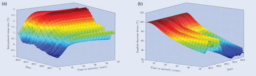
Figure 2. (a) Implied Black volatilities of caps from Bloomberg. (b) Caplet market prices in the single curve framework. Implied Black volatilities of caps from Bloomberg and caplet market prices on an annual basis for maturities ranging from 1 year to 20 years and for strike rates ranging from $1.00\mathrm{\%}$ to $10.00\mathrm{\%}$ in the single curve framework. The implied volatilities of caps in panel (a) consist of the market data on March 31st, 2017. The caplet market prices in panel (b) are recovered iteratively from the cap market prices on March 31st, 2017 through the single curve stripping procedure in equation (A4(A4) $\begin{array}{rl}& \mathrm{C}\mathrm{a}\mathrm{p}\mathrm{l}\mathrm{e}{\mathrm{t}}^{\mathrm{B}\mathrm{l}\mathrm{a}\mathrm{c}\mathrm{k}}(0,T_i,k,K,{\sigma }_i)\\ & =\mathrm{C}\mathrm{a}{\mathrm{p}}^{\mathrm{B}\mathrm{l}\mathrm{a}\mathrm{c}\mathrm{k}}(0,T_{i+1},k,K,\sigma )-\sum _{j=1}^{i+1}{Z}^0(0,T_j)\\ & \times \left(F^0(0,T_{j-1}^k,T_j^k)\mathrm{\Phi }\left({\mathrm{d}}_1\right({\sigma }_{j-1}\left)\right)-{\tilde{K}}_{j-1}^k\mathrm{\Phi }\left({\mathrm{d}}_2\right({\sigma }_{j-1}\left)\right)\right),\end{array}$(A4) ).

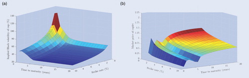
Figure 3. (a) OIS curves from Reuters. (b) Caplet market prices in the multiple curve framework. OIS curves from Reuters on a quarterly basis for maturities ranging from one quarter of a year to 30 years, and caplet market prices on an annual basis for maturities ranging from 1 year to 20 years and for strike rates ranging from $1.00\mathrm{\%}$ to $10.00\mathrm{\%}$ in the multiple curve framework. The OIS curves in panel (a) consist of the market rates on March 30th, 2012 up until April 28th, 2017. The caplet market prices in panel (b) are recovered iteratively from the cap market prices on March 31st, 2017 through the multiple curve stripping procedure in equation (A4(A4) $\begin{array}{rl}& \mathrm{C}\mathrm{a}\mathrm{p}\mathrm{l}\mathrm{e}{\mathrm{t}}^{\mathrm{B}\mathrm{l}\mathrm{a}\mathrm{c}\mathrm{k}}(0,T_i,k,K,{\sigma }_i)\\ & =\mathrm{C}\mathrm{a}{\mathrm{p}}^{\mathrm{B}\mathrm{l}\mathrm{a}\mathrm{c}\mathrm{k}}(0,T_{i+1},k,K,\sigma )-\sum _{j=1}^{i+1}{Z}^0(0,T_j)\\ & \times \left(F^0(0,T_{j-1}^k,T_j^k)\mathrm{\Phi }\left({\mathrm{d}}_1\right({\sigma }_{j-1}\left)\right)-{\tilde{K}}_{j-1}^k\mathrm{\Phi }\left({\mathrm{d}}_2\right({\sigma }_{j-1}\left)\right)\right),\end{array}$(A4) ).

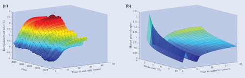
The results from the single curve bootstrap method in figure 1 highlight the facts that negative rates can occur nowadays and that market rates generally do not remain constant through time. Moreover, we observe a non-negligible spread between these 6-month tenor swap rates and the Overnight Indexed Swap (OIS) curves in figure 3(a), which thus seems to justify a multiple curve approach. After applying the stripping procedure in the single curve framework, the skewed shape of the volatility surface is also easily recognised from the implied Black volatilities of caps on March 31st, 2017 in figure 2(a). Besides that, a highly irregular structure of the caplet market prices is observed in figure 2(b) for short maturities and a quite smooth, upward sloping structure for long maturities. This irregularity is even more severe in the multiple curve approach in figure 3(b), since we account for the different tenor structure of caps with short maturities in this framework that contains a more frequent payment stream. Although it is tempting to say that this irregular structure arises due to the adopted interpolation schemes, this is in fact inherent in the dataset. This irregular structure appears to be caused by the occurrence of negative interest rates in combination with the incompatibility of Black's model with such negative rates. An alternative framework that is compatible with such negative rates is given by Bachelier (1900), but this framework is inconsistent with the implied volatilities from Bloomberg used in this paper that are based on Black's model.

3.2. Optimisation schemes

While Eberlein et al. (2016) and Eberlein et al. (2019) provide a closed-form expression to price individual caplets, they avoid any assumptions on the underlying distribution of the driving Lévy process. Raible (2000) offers an extensive overview of all the different kinds of distributions that can be implemented in this case. While the class of Generalised Hyperbolic (GH) distributions can allow for an almost perfect fit to financial data, its subclass of the Normal Inverse Gaussian (NIG) distribution in Barndorff-Nielsen (1997) typically already provides sufficient flexibility to fit financial data while relying on fewer parameters (Beinhofer et al. 2011). In addition, this class of distributions has its characteristic function available in closed-form and is in fact so flexible that multidimensional driving processes do not have to be considered, but that a one-dimensional Lévy process is already sufficient (Eberlein and Kluge 2007). We therefore incorporate one-dimensional NIG distributed Lévy processes in the calibrations of the LFPM specifications in this paper.

The NIG distribution constitutes a class of distributions with four parameters, which was first proposed by Barndorff-Nielsen (1995). While this distribution formally depends on four parameters in total, one parameter is irrelevant for the pricing of options and can therefore be arbitrarily set to zero (Kluge 2005). The Brownian component $c_{\mathrm{N}\mathrm{I}\mathrm{G}}$ and the Lévy measure $F_{\mathrm{N}\mathrm{I}\mathrm{G}}^{T^{\ast }}\left(\mathrm{d}x\right)$ of the driving Lévy process can, in this case, be represented in terms of merely three parameters, namely by $\begin{array}{l}{c}_{\mathrm{N}\mathrm{I}\mathrm{G}}=0,\\ F_{\mathrm{N}\mathrm{I}\mathrm{G}}^{T^{\ast }}\left(\mathrm{d}x\right)=\frac{\vartheta \kappa }{\pi |x|}{K}_1\left(\kappa |x|\right)\exp \left(\gamma x\right)\mathrm{d}x,\end{array}$ where $K_{\mu }\left(x\right)={\int }_0^{\mathrm{\infty }}{u}^{\mu -1}{e}^{-\left(1/2\right)x(1/u+u)}\mathrm{d}u$ denotes the modified Bessel function of the second kind of order μ, and with $\kappa >0$, $|\gamma |<\kappa$ and $\vartheta >0$ (Rydberg 1997, Morales and Schoutens 2003).

Finally, to optimise the criterion function in equation (1(1) $\underset{x}{min}\sum _{k=1}^m\sum _{i=1}^{n-1}\sum _{j=1}^h{\left(\frac{\begin{array}{c}\mathrm{C}\mathrm{a}\mathrm{p}\mathrm{l}\mathrm{e}{\mathrm{t}}^{\mathrm{M}\mathrm{a}\mathrm{r}\mathrm{k}\mathrm{e}\mathrm{t}}(0,T_i,k,K_j)\\ -\mathrm{C}\mathrm{a}\mathrm{p}\mathrm{l}\mathrm{e}{\mathrm{t}}^{\mathrm{M}\mathrm{o}\mathrm{d}\mathrm{e}\mathrm{l}}(0,T_i,k,K_j;x)\end{array}}{\mathrm{C}\mathrm{a}\mathrm{p}\mathrm{l}\mathrm{e}{\mathrm{t}}^{\mathrm{M}\mathrm{a}\mathrm{r}\mathrm{k}\mathrm{e}\mathrm{t}}(0,T_i,k,K_{\mathrm{A}\mathrm{T}\mathrm{M}})}\right)}^2,$(1) ), this paper adopts the non-linear matlab function lsqnonlin. Moreover, to allow for an efficient calibration of the model specifications on a daily basis, the trapezoidal method is adopted to numerically approximate the three integrals in equation (3(3) $\begin{array}{rl}& \mathrm{C}\mathrm{a}\mathrm{p}\mathrm{l}\mathrm{e}\mathrm{t}(0,T_h,k,K)\\ & =\frac{{\tilde{K}}_h^k{P}_z^0(0,T_{h+1})}{2\pi }{\int }_{\mathbb{R}}\left\{{\left(\frac{F^0(0,T_h^k,T_{h+1}^k)}{{\tilde{K}}_h^k}\right)}^{R+\mathrm{i}u}\right.\\ & \times \exp \left({\int }_0^{T_h}{\int }_{\mathbb{R}}{e}^{x{\mathrm{\Lambda }}^{0,h+1}\left(s\right)}\left[\left(e^{(R+\mathrm{i}u)x{\lambda }^0(s,T_h)}-1\right)\right.\right.\\ & -\left.\left.(R+\mathrm{i}u)\left(e^{x{\lambda }^0(s,T_h)}-1\right)\right]F_s^{T^{\ast }}\left(\mathrm{d}x\right)\mathrm{d}s\phantom{{\int }_0^{T_h}}\right)\\ & \times \left.\phantom{{\left(\frac{F^0(0,T_h^k,T_{h+1}^k)}{{\tilde{K}}_h^k}\right)}^{R+\mathrm{i}u}}\exp \left({\int }_0^{T_h}\frac{c_s}{2}(R+\mathrm{i}u)(R+\mathrm{i}u-1){\lambda }^0(s,T_h{)}^2\mathrm{d}s\right)\right\}\\ & \times \frac{\mathrm{d}u}{(R+\mathrm{i}u)(R+\mathrm{i}u-1)},\end{array}$(3) ). This method can be implemented quite easily through the matlab function trapz, with the optimisation options specified in table 7. More importantly, this numerical approximation significantly eases the computational burden and ensures tractability in the LFPM.

However, this optimisation routine might be sensitive to its initial starting values, since the criterion function could have multiple local minima. To resolve this issue, the non-linear optimisation scheme is first performed for different starting values and boundaries together with simulated annealing, which offers a more global optimisation scheme than lsqnonlin at the expense of a higher computational burden. This, in turn, returns the estimated parameters that match the smallest value of the criterion function and leads to somewhat more sophisticated starting values for the calibrations. Even though this method does not ensure that the global minimum of the non-linear criterion function is acquired, it does make the optimisation routine less sensitive to its initial starting values and more robust to local minima. As a result, the initial starting values and boundaries reported in table 8 are adopted in the calibrations of the model specifications with lsqnonlin.

4. Empirical performance analysis

4.1. Goodness-of-fit

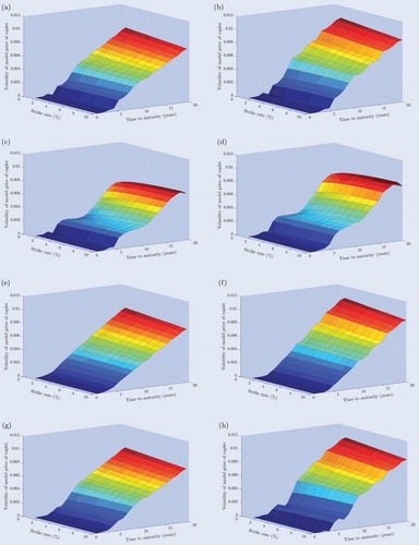
Based on the relevant market data on March 31st, 2017 and the optimisation methodology described earlier, the goodness-of-fit of each separate model specification is deduced. While table 1 displays the goodness-of-fit for each model specification, table A3 reports the corresponding calibrated parameters. Moreover, the caplet prices of each deterministic model specification and the respective absolute pricing errors in terms of the implied Black volatilities of the LEV model specifications are presented in figures 4 and 5, respectively, for both the single and multiple curve framework. The results of the other model specifications are available upon request.

Figure 4. (a) Single curve - CEV - Deterministic. (b) Multiple curve - CEV - Deterministic. (c) Single curve - DCEV - Deterministic. (d) Multiple curve - DCEV - Deterministic. (e) Single curve - LEV - Deterministic. (f) Multiple curve - LEV - Deterministic. (g) Single curve - QV - Deterministic. (h) Multiple curve - QV - Deterministic. Individual caplet prices of each deterministic single and multiple curve model specification for maturities ranging from 1 year to 20 years and for strike rates ranging from 1.00% to 10.00%. The prices are obtained after calibration to the market data on March 31st, 2017.

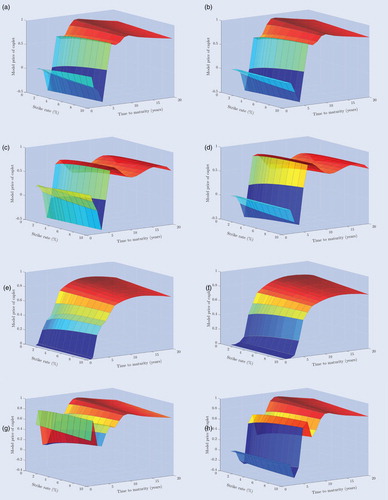
Figure 5. (a) Single curve - LEV - Deterministic. (b) Multiple curve - LEV - Deterministic. (c) Single curve - LEV - Random. (d) Multiple curve - LEV - Random. Absolute pricing errors of individual caplets of the single and multiple curve LEV model specifications for maturities ranging from 1 year to 20 years and for strike rates ranging from $1.00\mathrm{\%}$ to $10.00\mathrm{\%}$. The pricing errors are expressed in implied Black volatilities and are obtained after calibration to the market data on March 31st, 2017.

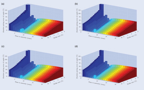
Table 1. Goodness-of-fit of each single and multiple curve model specification after calibration on March 31st, 2017. The values of this performance criterion are obtained through the optimisation options specified in table 8.

	Deterministic				Random
Framework	CEV	DCEV	LEV	QV	CEV	DCEV	LEV	QV
Single curve	34.5445	48.2524	19.0228	25.9572	34.7094	48.2524	18.9674	29.4501
Multiple curve	36.5929	49.9099	21.6844	33.6905	36.5922	49.9099	21.4628	33.6993

Although the differences between all model specifications seem rather modest, two of them appear to be superior to the others. Table 1, for instance, shows that the LEV specification slightly outperforms the other volatility functions. This comes as no surprise, since the LEV specification involves more parameters than the CEV and the QV specification, and adopts a more sophisticated functional form than the DCEV specification. It therefore appears that we can confirm the claim made by Eberlein and Kluge (2007), who argue that the LEV function already provides a sufficiently flexible structure to capture the implied volatility surface of caplets. The single curve framework additionally seems to slightly outperform its multiple curve analogue for all volatility specifications, where the most notable difference is observed for the QV function. Besides that, tables 1 and 9 reveal that the additional feature of random breakpoints has hardly any benefits over simply assuming deterministic breakpoints in both the single and multiple curve framework, and that deterministic breakpoints are in fact adopted in the random model specifications as well.

This preliminary conclusion is confirmed by the caplet model prices and the corresponding absolute pricing errors. Figure 4 shows that the caplet prices in the deterministic CEV and DCEV specification are highly irregular and lead to substantially negative prices, while the LEV and the QV specification result in a more natural, upward sloping structure. Moreover, the LEV specifications produce a particularly smooth surface of caplet prices, with strictly positive prices for each caplet and with higher prices for longer maturities. These observations seem to be persistent in both the single and multiple curve framework, where almost the same pricing surfaces arise except for short maturities in the QV specification. However, all the absolute pricing errors tend to follow roughly the same pattern as the LEV model specifications in figure 5. This pattern where larger pricing errors occur for short maturities and low strike rates than for long maturities and high strike rates, is mainly due to the irregular structure of the caplet market prices. The occurrence of negative interest rates and the incompatibility of Black's model with such negative rates thus seem to have a more severe effect on the short-term and for low strike rates than on the long-term and for high strike rates, where in fact quite regular and smooth prices arise. It thus indeed seems that the LFPM with the LEV specification, both in the single and multiple curve framework, is superior and that allowing for random breakpoints only offers a marginal improvement.

4.2. Parameter stability

An interesting question is now whether significantly different results are found if the calibrations were performed on other dates or in terms of the parameter stability. By adopting the same optimisation strategy as in the previous section with the relevant market data on March 30th, 2012 up until March 31st, 2017, the caplet prices of all eight model specifications and their absolute pricing errors are obtained in both the single and multiple curve framework. The parameter stability, or the volatility of the resulting parameter estimates, is presented in table 2 for each model specification separately. Tables 10 and 11 report the average goodness-of-fit together with its volatility and the average parameter estimates, respectively. In addition, it is investigated whether these calibrations lead to any substantial changes in the model prices, where the volatilities of the average caplet prices of the deterministic model specifications are displayed in figure A3. The volatilities of the average absolute pricing errors of the LEV specification in terms of the implied Black volatilities are shown in figure A4. The results of the other model specifications are available upon request.

Table 2. Parameter stability of each single and multiple curve model specification after calibration on March 30th, 2012 up until March 31st, 2017. The volatilities are obtained by assessing the standard errors of the parameter estimates retrieved through the optimisation options specified in table 8. Note that it is assumed that $(\varphi ,\psi )=(1,5)$ in the deterministic model specifications, and that they therefore have no standard deviation.

	Deterministic				Random
Parameter	CEV	DCEV	LEV	QV	CEV	DCEV	LEV	QV
Single curve framework
ϕ	–	–	–	–	0.0000	0.0000	0.0000	0.0000
ψ	–	–	–	–	0.0000	0.0000	0.0000	0.0000
α	0.0096	0.0185	0.3883	1.5983	0.0092	0.0179	0.3936	1.7357
β	–	0.0091	0.0633	–	–	0.0093	0.0685	–
ω	–	0.0088	0.0634	2.5670	–	0.0079	0.0592	2.6435
${\kappa }_S$	0.2954	0.1208	1.8521	0.7188	0.3260	0.0945	1.9082	0.8367
${\gamma }_S$	0.6129	0.5357	3.0572	1.0811	0.5550	0.3877	2.4708	1.1184
${\vartheta }_S$	$3.2249\times {10}^{-7}$	$5.9081\times {10}^{-5}$	0.0016	$7.2461\times {10}^{-7}$	$3.0736\times {10}^{-7}$	$5.3727\times {10}^{-5}$	0.0059	$8.3170\times {10}^{-5}$
${\kappa }_M$	0.1328	2.1267	0.3413	0.3591	0.1325	0.1185	0.2905	0.0274
${\gamma }_M$	0.1704	3.3157	0.3030	0.6437	0.1185	0.5232	0.2314	0.0228
${\vartheta }_M$	$1.9645\times {10}^{-5}$	0.0594	0.0029	0.0138	$1.1677\times {10}^{-5}$	0.0683	0.0012	0.0174
${\kappa }_L$	0.0784	0.0948	0.8275	0.1595	0.0538	0.0943	0.6387	0.1521
${\gamma }_L$	0.1043	0.4628	1.0198	1.0326	0.0479	0.5179	0.6035	0.9614
${\vartheta }_L$	0.0014	1.9731	$2.2881\times {10}^{-6}$	0.0172	0.0014	1.9105	$4.6708\times {10}^{-7}$	0.0187
Multiple curve framework
ϕ	–	–	–	–	0.0000	0.0000	0.0000	0.0000
ψ	–	–	–	–	0.0000	0.0000	0.0000	0.0000
α	0.0126	0.0115	0.2965	1.7752	0.0137	0.0115	0.2904	1.8911
β	–	0.0065	0.0591	–	–	0.0070	0.0593	–
ω	–	0.0067	0.0449	2.8938	–	0.0064	0.0445	3.2805
${\kappa }_S$	0.4066	0.1149	0.6767	0.9070	0.4465	0.1236	0.6058	0.8563
${\gamma }_S$	0.8342	0.4918	1.1166	1.3037	0.6671	0.5049	0.7690	0.9634
${\vartheta }_S$	$1.4332\times {10}^{-6}$	0.0001	0.0008	0.0003	$6.7308\times {10}^{-7}$	0.0001	0.0009	$1.4117\times {10}^{-6}$
${\kappa }_M$	0.0782	1.9755	0.1716	0.5282	0.0254	0.0362	0.1548	0.0219
${\gamma }_M$	0.1008	2.7018	0.1545	0.6583	0.0214	0.1996	0.1216	0.0187
${\vartheta }_M$	$2.0573\times {10}^{-5}$	0.0338	$4.6632\times {10}^{-5}$	0.0183	$1.1276\times {10}^{-5}$	0.0318	$4.7500\times {10}^{-5}$	0.0251
${\kappa }_L$	0.0747	0.0838	0.8034	0.1755	0.0640	0.0868	0.7962	0.1754
${\gamma }_L$	0.0998	0.5661	1.0018	0.9588	0.0605	0.4831	0.6831	0.9787
${\vartheta }_L$	0.0021	1.7122	$6.0544\times {10}^{-7}$	0.0296	0.0045	1.2131	$6.8233\times {10}^{-7}$	0.0240

While the calibrations indicate that two model specifications are again superior to the others, somewhat different results are now in fact found. The average goodness-of-fit and its volatility in table 10, for instance, show that each model specification has a considerably worse fit to the market data than on March 31st, 2017, and that these model fits experience large amounts of volatility. This vast decrease in model fit is due to the irregular pattern inherent in the market prices of short-term caplets. Even though the LEV specification and the DCEV specification seem to substantially outperform the other volatility functions, all model specifications thus appear to be unsuccessful in appropriately incorporating this irregularity in the caplet market prices. However, this decrease in model fit is substantially lower in the multiple curve framework than in the single curve framework, where the resulting average goodness-of-fit is five to six times as small. It therefore seems more likely that the market adopts a multiple curve approach to value the caplets than a single curve approach. Furthermore, the parameter stability of each model specification in table 2 and the means of the estimated parameters in table 11 seem to support this claim. Based on the parameter stability of the eight model specifications, the resulting parameter estimates seem to be, overall, quite stable. This suggests that it is expected that, on average, more or less the same structure of caplet prices is obtained for each model specification as on March 31st, 2017.

On average, we indeed find qualitatively the same caplet prices for each model specification, and figure A3 demonstrates that the caplet prices in the deterministic case are in fact the most volatile on the short-term. We additionally find that the caplet prices with one or two years of maturity are substantially less volatile in the multiple curve framework, but that those with four to five years of maturity actually display more volatility in this framework. However, the calibrations do seem to result in a somewhat less smooth structure of caplet prices for the LEV specification, although it does still lead to strictly positive prices and preserves the upward sloping relationship with respect to the time to maturity. Similarly, the pricing errors display almost no discrepancy across model specifications and follow the same pattern as on March 31st, 2017. The argument of Beinhofer et al. (2011) that the class of GH distributions, and in particular the NIG distribution, already provides enough flexibility to fit financial data therefore seems to uphold in this analysis, since more or less the same pricing errors result for each model specification in both the single and multiple curve framework. Besides that, the volatilities of these pricing errors for the LEV model specifications in figure A4 indeed exhibit a degree of variation along the time to maturity. In other words, substantially larger pricing errors are in fact observed for short maturities than for long maturities as a result of the irregularity inherent in the market data. However, since risk management is mainly concerned with longer maturities, this does not pose any severe issues.

4.3. Out-of-sample pricing

Up to now, the robustness of the earlier results with respect to small market changes have been left largely unanswered, while, from a risk management perspective, such changes are essential for an ALM study. To adequately address the robustness of the results, this paper inspects the out-of-sample pricing of the eight model specifications for April 3rd, 2017 up until April 28th, 2017 after calibration on March 31st, 2017 in both the single and multiple curve framework. While the average goodness-of-fit and its volatility are presented for each model specification in table 3, figure 6 reports the volatilities of the average absolute out-of-sample pricing errors for the LEV specifications. In addition, figure A5 displays the volatilities of the average caplet prices in the deterministic case. The results of the other model specifications are available upon request.

Figure 6. (a) Single curve - LEV - Deterministic. (b) Multiple curve - LEV - Deterministic. (c) Single curve - LEV - Deterministic. (d) Multiple curve - LEV - Random. Volatilities of the absolute out-of-sample pricing errors of individual caplets of the single and multiple curve LEV model specifications for maturities ranging from 1 year to 20 years and for strike rates ranging from $1.00\mathrm{\%}$ to $10.00\mathrm{\%}$. The volatilities are expressed in implied Black volatilities and are obtained after calibration to the market data on March 31st, 2017 for April 3rd, 2017 up until April 28th, 2017.

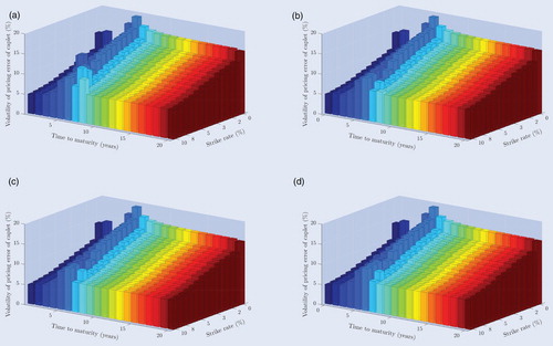
Table 3. Average goodness-of-fit for April 3rd, 2017 up until April 28th, 2017 of each single and multiple curve model specification as well as its standard deviation in parentheses after calibration on March 31st, 2017. The values of this performance criterion are obtained through the optimisation options specified in table 8.

	Deterministic				Random
Framework	CEV	DCEV	LEV	QV	CEV	DCEV	LEV	QV
Single curve	40.3654	51.1501	23.8000	29.5975	39.5650	51.1501	24.6024	35.8822
	(6.5067)	(7.5479)	(8.1418)	(5.4990)	(6.2354)	(7.5479)	(8.6370)	(5.6975)
Multiple curve	42.3921	61.4927	28.7093	45.4880	42.4064	61.4927	28.4590	45.1684
	(6.4433)	(10.7317)	(9.3501)	(10.3286)	(6.4492)	(10.7317)	(9.2632)	(10.0810)

Even though the overall differences seem to be quite modest, two of the model specifications again appear to be superior to the others. Qualitatively the same results are in fact found for the out-of-sample pricing of the model specifications as for the goodness-of-fit in section 4.1. Table 3, for instance, shows that the LEV specification, in general, slightly outperforms the other volatility functions in terms of the goodness-of-fit. More specifically, the results indicate that the CEV and the DCEV specification again result in a much worse fit than the LEV specification, that the QV function produces only a slightly worse fit and that the single curve approach slightly outperforms the multiple curve approach in all specifications. In addition, the LEV or DCEV specification tends to lead to the most volatile goodness-of-fit, whereas the QV specification introduces the most stable or volatile goodness-of-fit in the single or multiple curve framework, respectively. In contrast to the analysis in section 4.1, the possibility of random breakpoints now typically leads to a worse goodness-of-fit and to a larger volatility of this fit, indicating a degree of overfitting, and this relation seems to be particularly persistent for the LEV and the QV specification in the single curve approach. However, these differences appear to arise due to the flexibility that the additional parameters in the functional form of the volatility function and in the Lévy measure of the driving process offer. Despite these drawbacks, the LEV specification continues to be the superior model specification, although allowing for random breakpoints now seems to come at a considerable cost.

Besides the goodness-of-fit, qualitatively the same patterns are also found in the out-of-sample caplet prices and their absolute pricing errors. The structure of the average caplet prices is again quite irregular and very similar to the caplet prices in figure 4. Likewise, random breakpoints lead to slightly smoother out-of-sample caplet prices, although this effect appears to be minuscule at best. In addition, the volatilities of these caplet prices in the deterministic case in figure A5 are all rather modest and exhibit an upward sloping relationship with respect to the time to maturity. The DCEV specification seems to be the most stable in terms of the resulting caplet prices, but since the volatilities of the out-of-sample caplet prices are all remarkably small, this result is negligible.

However, the average absolute pricing errors and their volatilities barely vary across single and multiple curve model specifications, similarly to the pricing errors in figure 5. This is again due to the irregular structure of the caplet market prices that arises as a result of the occurrence of negative interest rates and the incompatibility of Black's model with such negative rates. The volatilities of these pricing errors for the LEV specifications in figure 6 are actually larger for long maturities than for short maturities, which does not come as a surprise since the out-of-sample caplet prices already tended to be more volatile for long maturities than for short maturities. All things considered, though, each model specification seems to lead to similar out-of-sample pricing errors in both the single and multiple curve framework, and a comparison of these errors does not contribute much to the empirical performance analysis of the model specifications.

5. Summary and concluding remarks

The main research objective in this paper was to discover how a single curve stochastic term structure model can best be constructed and estimated for Asset Liability Management purposes, and how it compares to its multiple curve analogue. Because of the increasing concern for negative interest rates and the risk of this low, negative interest rate environment for financial institutions, the urgency of accounting for the current state of financial markets has risen sharply. The stochastic interest rate model thus not only had to capture the prices of popular derivatives traded in the market, but had to allow for substantially negative interest rate scenarios as well. By implementing such a model in an ALM study, financial institutions are able to address this interest rate risk and it therefore enables them to more globally assess their financial stability.

Based on a range of criteria, a literature review was made of single curve stochastic interest rate models in terms of their adequacy for an ALM study (appendix 1). At first sight it seemed that some of the most widely adopted short-rate models in practice may have some rather undesirable properties in the negative interest rate environment that we currently observe. More importantly, this review suggested that, among single curve stochastic interest rate models, especially the Lévy Forward Price Model seems to have appropriate characteristics for ALM purposes. This LFPM was further implemented with four types of deterministic volatility functions under a piecewise homogeneity restriction on the driving one-dimensional Lévy process, with both deterministic and random breakpoints and in both the single and multiple curve framework. Moreover, an explicit parametrisation of this restriction was provided in terms of the canonical representations of the driving piecewise homogeneous Lévy processes. A concatenation of these processes was additionally introduced to further enhance the smoothness of the driving process as a whole.

Following this explicit parametrisation, an optimisation routine was provided for calibrating the LFPM. This routine described how to explicitly obtain the market prices of interest rate caplets from a stripping procedure and the bootstrap method in both the single and multiple curve framework. With these market data, an empirical performance analysis was made of the single and multiple curve LFPM in terms of three distinct performance measures including the goodness-of-fit, the parameter stability and the out-of-sample pricing. From this, we concluded that the Linear-Exponential Volatility specification yields, by far, the best results and outperforms the other deterministic volatility functions in both the single and multiple curve approach. Moreover, while random breakpoints in the piecewise homogeneous Lévy processes seemed to offer only some minor benefits for the goodness-of-fit and essentially none for the parameter stability, it in fact severely worsened the out-of-sample pricing of the LEV specification in the single curve framework due to a degree of overfitting. More importantly, it seemed more likely that the market adopts the multiple curve approach to value the interest rate caplets, since this framework led, on average, to a substantially better goodness-of-fit than the single curve framework. The comparative analysis in this paper therefore indicates that financial institutions can best adopt the multiple curve LFPM in their ALM studies with the LEV specification and with deterministic breakpoints.

Besides these three performance criteria, future studies could also evaluate more sophisticated criteria to investigate whether this would lead to qualitatively the same results. One example is the jackknife resampling method, which can be used to assess the robustness of the results with respect to the inclusion of longer maturities and additional strike rates. More complex approaches that involve consistent recalibration, a non-parametric kernel regression, a Principal Components Analysis or the General Method of Moments could be adopted in further research as well to validate the conclusions of this research. To assess the accuracy, future studies could focus on additional robustness checks of the optimisation options adopted in this paper. Additionally, it would be worth investigating whether the irregularity in the caplet market prices would reduce if the implied volatilities were based on Bachelier's framework that is, unlike Black's model, consistent with negative interest rates. Such a framework could improve the empirical performance of the LFPM considerably, and hence the risk management practices of financial institutions.

Acknowledgements

The author would like to thank the anonymous referees for valuable suggestions which greatly improved the paper.

Disclosure statement

No potential conflict of interest was reported by the author.

Appendix 1. Model selection for ALM studies using a single curve

Despite the extensive literature on single curve stochastic term structure models, many stochastic interest rate models may be inappropriate for Asset Liability Management purposes. This appendix therefore focuses on what criteria these models should meet for an ALM study.

Although there are many classes of single curve stochastic interest rate models, not all possess desirable features for an ALM study. There are several characteristics that label a stochastic term structure model as appropriate for simulating interest rate scenarios, including:

1. Long-term rates - The model should be able to capture the entire yield curve to fully describe the evolution of the assets and liabilities of a financial institution.

2. Market consistency - An exact fit to the current term structure of interest rates should be ensured by the model, while retaining its compatibility to discrete, observable market rates.

3. Negative rates - The persistence of negative interest rates in financial markets is apparent. The model should therefore be able to sufficiently cope with this interest rate environment.

4. Mean reversion - Historical data highlight the fact that interest rates tend to go down when high and to go up when low. In other words, interest rates typically revert to a mean level.

5. Arbitrage-free - Derivatives should be priced such that arbitrage opportunities do not exist.

6. Curve variation - The model should lead to variation in parallel shifts, steepness and curvature to provide plausible interest rate scenarios.

7. Tractability - Analytical, closed-form pricing formulas lead to a more tractable and reliable model, since the calibrations consist of calculating thousands of prices of popular derivatives.

With these criteria and the overview from section 1, the single curve stochastic term structure models can be compared for ALM studies. The results of this comparison are shown in table 4.

Table A1. Model selection for ALM studies showing which classes of single curve stochastic interest rate models satisfy what types of model selection criteria. A check/cross mark means that the criterion is only met under specific conditions.

Model	Short-rate	HJM	Affine short-rate	LMM/SMM	LFPM
Long-term rates	×	✓	×	✓	✓
Market consistency	×	×	×	✓	✓
Negative rates	✓/×	✓	✓/×	✓/×	✓
Mean reversion	✓	✓	✓	✓	✓
Arbitrage-free	✓/×	✓	✓	✓	✓
Curve variation	✓	✓	✓	✓	✓
Tractability	✓/×	×	✓	✓/×	✓

While the LFPM satisfies all selection criteria, all the other classes of models always seem to violate at least one crucial criterion. This implies that from the wide range of available single curve models, especially the LFPM seems suitable to implement in an ALM study.

Appendix 2. Construction of the single curve forward price process

While section 2.1.1 only briefly discussed the importance of assumptions ($\mathbb{E}\mathbb{M}$), ($\mathbb{D}\mathbb{V}$) and ($\mathbb{B}\mathbb{P}$), their relevance will become clearer from the derivation of the single curve framework in this appendix. To begin with, let $0=T_0<T_1<\cdots <T_{n-1}<T_n=T^{\ast }$ denote a discrete tenor structure of maturities and set ${\delta }_i=T_i-T_{i-1}$ equal to the time between these maturities. This, in turn, allows for $F(t,T_i,T_{i+1})=\frac{P_z(t,T_i)}{P_z(t,T_{i+1})}\text{for every }i\in \{0,\dots ,n-1\}$ as the more formal definition of the forward price process $F(\cdot ,T_i,T_{i+1})$. In reality, these future zero coupon bond prices are unknown, and a different expression for the forward price is thus required.

One way to construct the forward price process is through backward induction, where the process with the longest maturity is regarded first. For this forward price $F(\cdot ,T_{n-1},T^{\ast })$, we postulate that (A1) $F(t,T_{n-1},T^{\ast })=F(0,T_{n-1},T^{\ast })\exp \left({\int }_0^t\lambda (s,T_{n-1})\mathrm{d}{L}_s^{T^{\ast }}\right),$(A1) subject to the initial condition $F(0,T_{n-1},T^{\ast })=\frac{P_z(0,T_{n-1})}{P_z(0,T^{\ast })}.$ At this point, the main objective in this construction is to specify the drift characteristic $b^{T^{\ast }}$ such that the forward price process $F(\cdot ,T_{n-1},T^{\ast })$ must be a martingale with respect to its forward measure ${\mathbb{P}}_{T^{\ast }}$, or $\begin{array}{rl}& {\int }_0^t⟨\lambda (s,T_{n-1}),b_s^{T^{\ast }}⟩\mathrm{d}s\\ & =-\frac{1}{2}{\int }_0^t⟨\lambda (s,T_{n-1}),c_s\lambda (s,T_{n-1})⟩\mathrm{d}s\\ & -{\int }_0^t{\int }_{{\mathbb{R}}^d}\left(e^{⟨\lambda (s,T_{n-1}),x⟩}-1-⟨\lambda (s,T_{n-1}),x⟩\right){\nu }^{T^{\ast }}\left(\mathrm{d}s,\mathrm{d}x\right),\end{array}$ where ${\nu }^{T^{\ast }}(\mathrm{d}s,\mathrm{d}x):=F_s^{T^{\ast }}\left(\mathrm{d}x\right)\mathrm{d}s$ denotes the compensator of the random measure ${\mu }^L$ associated with the jumps of the Lévy process $L^{T^{\ast }}$. Moreover, applying Lemma 2.6 in Kallsen and Shiryaev (2002) to express the forward price in equation (A1(A1) $F(t,T_{n-1},T^{\ast })=F(0,T_{n-1},T^{\ast })\exp \left({\int }_0^t\lambda (s,T_{n-1})\mathrm{d}{L}_s^{T^{\ast }}\right),$(A1) ) as the stochastic exponential of a local martingale yields $F(t,T_{n-1},T^{\ast })=F(0,T_{n-1},T^{\ast }){\mathcal{E}}_t\left(H\right(\cdot ,T_{n-1}\left)\right)$ with (A2) $\begin{array}{rl}H(t,T_{n-1})& ={\int }_0^t\sqrt{c_s}\lambda (s,T_{n-1})\mathrm{d}{W}_s^{T^{\ast }}\\ & +{\int }_0^t{\int }_{{\mathbb{R}}^d}\left(e^{⟨\lambda (s,T_{n-1}),x⟩}-1\right)\left({\mu }^L-{\nu }^{T^{\ast }}\right)\left(\mathrm{d}s,\mathrm{d}x\right).\end{array}$(A2) Note that this local martingale $H(\cdot ,T_{n-1})$ is in fact a time-inhomogeneous Lévy process as well. Eberlein et al. (2005) prove that, in this particular case where the stochastic exponential of a process is both a local martingale and a time-inhomogeneous Lévy process, it is not just a local martingale but actually a martingale as well. As a consequence, the forward price process $F(\cdot ,T_{n-1},T^{\ast })$ is a martingale itself with respect to its forward measure ${\mathbb{P}}_{T^{\ast }}$.

This conclusion that the forward price process $F(\cdot ,T_{n-1},T^{\ast })$ is in fact also a martingale, has a crucial implication for the remaining part of this derivation. This result actually allows for a definition of the forward martingale measure associated with the maturity date $T_{n-1}$, by $\frac{\mathrm{d}{\mathbb{P}}_{T_{n-1}}}{\mathrm{d}{\mathbb{P}}_{T^{\ast }}}=\frac{F(T_{n-1},T_{n-1},T^{\ast })}{F(0,T_{n-1},T^{\ast })}={\mathcal{E}}_{T_{n-1}}\left(H\right(\cdot ,T_{n-1}\left)\right).$ Moreover, Girsanov's Theorem for semi-martingales, see for instance Theorem III.3.24 in Jacod and Shiryaev (2003), can now be applied to identify the two previsible processes β and Y from equation (A2(A2) $\begin{array}{rl}H(t,T_{n-1})& ={\int }_0^t\sqrt{c_s}\lambda (s,T_{n-1})\mathrm{d}{W}_s^{T^{\ast }}\\ & +{\int }_0^t{\int }_{{\mathbb{R}}^d}\left(e^{⟨\lambda (s,T_{n-1}),x⟩}-1\right)\left({\mu }^L-{\nu }^{T^{\ast }}\right)\left(\mathrm{d}s,\mathrm{d}x\right).\end{array}$(A2) ) that describe this change of measure, by recognising that $\text{β}\left(s\right)=\lambda (s,T_{n-1})\mathrm{a}\mathrm{n}\mathrm{d}Y(s,x)=\exp \left(⟨\lambda (s,T_{n-1}),x⟩\right).$ As a consequence, $\begin{array}{rl}{W}_t^{T_{n-1}}& :=W_t^{T^{\ast }}-{\int }_0^t\sqrt{c_s}\lambda (s,T_{n-1})\mathrm{d}s,\\ {\nu }^{T_{n-1}}(\mathrm{d}t,\mathrm{d}x)& :=\exp \left(⟨\lambda (t,T_{n-1}),x⟩\right)F_t^{T^{\ast }}\left(\mathrm{d}x\right)\mathrm{d}t\end{array}$ denote a standard Brownian motion under its forward measure ${\mathbb{P}}_{T_{n-1}}$ and the ${\mathbb{P}}_{T_{n-1}}$-compensator of ${\mu }^L$, respectively. This yields the ${\mathbb{P}}_{T_{n-1}}$-canonical representation of the time-inhomogeneous Lévy process $L^{T^{\ast }}$, given by $\begin{array}{rl}{L}_t^{T^{\ast }}& ={\int }_0^t{\hat{b}}_s\mathrm{d}s+{\int }_0^t\sqrt{c_s}\mathrm{d}{W}_s^{T_{n-1}}\\ & +{\int }_0^t{\int }_{{\mathbb{R}}^d}x\left({\mu }^L-{\nu }^{T_{n-1}}\right)(\mathrm{d}s,\mathrm{d}x),\end{array}$ where the deterministic drift coefficient $\hat{b}$ can be calculated with Girsanov's Theorem.

By repeating this scheme for all other maturities in the discrete tenor structure, expressions are in fact found for the forward price processes $F(\cdot ,T_i,T_{i+1})$ for $i\in \{1,\dots ,n-2\}$, and for their corresponding forward measures ${\mathbb{P}}_{T_i}$ for $i\in \{2,\dots ,n-2\}$. In other words, a forward price model is obtained by backward induction, where the forward price process $F(\cdot ,T_i,T_{i+1})$ is defined as $F(t,T_i,T_{i+1})=F(0,T_i,T_{i+1})\exp \left({\int }_0^t\lambda (s,T_i)\mathrm{d}{L}_s^{T_{i+1}}\right),$ with $\begin{array}{rl}{L}_t^{T_{i+1}}& ={\int }_0^t{b}_s^{T_{i+1}}\mathrm{d}s+{\int }_0^t\sqrt{c_s}\mathrm{d}{W}_s^{T_{i+1}}\\ & +{\int }_0^t{\int }_{{\mathbb{R}}^d}x\left({\mu }^L-{\nu }^{T_{i+1}}\right)(\mathrm{d}s,\mathrm{d}x).\end{array}$ In this canonical representation of the driving Lévy process, $\begin{array}{rl}{W}_t^{T_{i+1}}& =W_t^{T^{\ast }}-{\int }_0^t\sqrt{c_s}\sum _{j=i+1}^{n-1}\lambda (s,T_j)\mathrm{d}s,\\ {\nu }^{T_{i+1}}(\mathrm{d}t,\mathrm{d}x)& =\exp \left(\sum _{j=i+1}^{n-1}⟨\lambda (t,T_j),x⟩\right)F_t^{T^{\ast }}\left(\mathrm{d}x\right)\mathrm{d}t\end{array}$ denote a standard Brownian motion under its forward measure ${\mathbb{P}}_{T_{i+1}}$ and the ${\mathbb{P}}_{T_{i+1}}$-compensator of ${\mu }^L$, respectively. Finally, the drift characteristic $b^{T_{i+1}}$ must satisfy $\begin{array}{rl}& {\int }_0^t⟨\lambda (s,T_i),b_s^{T_{i+1}}⟩\mathrm{d}s\\ & =-\frac{1}{2}{\int }_0^t⟨\lambda (s,T_i),c_s\lambda (s,T_i)⟩\mathrm{d}s\\ & -{\int }_0^t{\int }_{{\mathbb{R}}^d}\left(e^{⟨\lambda (s,T_i),x⟩}-1-⟨\lambda (s,T_i),x⟩\right){\nu }^{T_{i+1}}\left(\mathrm{d}s,\mathrm{d}x\right).\end{array}$ Note that the driving processes $L^{T_i}$ are more or less the same for each maturity $T_i$, apart from their deterministic drift terms, and that they all remain time-inhomogeneous under their respective forward measure. It is exactly this property of the LFPM that allows for analytical pricing formulas of caps and individual caplets, and for the LFPM to retain its tractability.

Appendix 3. Recovery of discount factors and caplet prices

The discount factors and caplet prices shown in section 3.1 are not directly quoted by the market, but need to be recovered indirectly instead. This appendix explains how the discount factors and caplet prices can be obtained from the bootstrap method mentioned in Veronesi (2010) or Ametrano and Bianchetti (2013) and the stripping procedure outlined in Brigo and Mercurio (2006) or Bianchetti and Carlicchi (2012) in the single or multiple curve framework, respectively, with data from Bloomberg and Reuters.

A.1. Bootstrap-implied discount factors

Despite their significance in financial markets, discount factors are not directly quoted by the market. One way to still recover these discount factors is through the bootstrap method, which iteratively retrieves the discount factors from coupon bearing bonds one maturity at a time (Veronesi 2010, Ametrano and Bianchetti 2013). More importantly, the risk-free discount factors can be bootstrapped from the term structure of swap rates as well, which are readily available in the market through, for example, Bloomberg or Reuters. The bootstrap method coincides, in this case, with (A3) $Z^0(t,T_i)=\left\{\begin{array}{ll}\frac{1}{1+\frac{s_{\mathrm{\Delta }}^0(t,T_1)}{\mathrm{\Delta }}}& \text{for }i=1\\ \frac{1-\frac{s_{\mathrm{\Delta }}^0(t,T_i)}{\mathrm{\Delta }}\sum _{j=1}^{i-1}{Z}^0(t,T_j)}{1+\frac{s_{\mathrm{\Delta }}^0(t,T_i)}{\mathrm{\Delta }}}& \text{for }i\in \{2,3,\dots ,n\}\end{array}\right.,$(A3) where $s_{\mathrm{\Delta }}^0(t,T_i)$ denotes the Δ-compounded swap rate at date t with time to maturity $T_i$ and Δ the (time-invariant) payment frequency. These swap rates $s_{\mathrm{\Delta }}^0(t,T_i)$ typically have the 6-month EURIBOR rate as their underlying index in the single curve framework, whereas the multiple curve approach usually takes the overnight rate as the underlying index.

However, this is only valid for the basic curve while the risky tenor-dependent curves need to be bootstrapped as well in the multiple curve approach. In case of a standard deposit contract, Ametrano and Bianchetti (2013) show that the risky discount factors can be retrieved through $Z^0(t,T_i^k)=\frac{1}{1+\frac{s_{{\mathrm{\Delta }}^k}^0(t,T_i^k)}{{\mathrm{\Delta }}^k}}\text{for }i\in \{1,2,\dots ,n\},$ where $s_{{\mathrm{\Delta }}^k}^0(t,T_i^k)$ now denotes the ${\mathrm{\Delta }}^k$-compounded deposit rate at date t with maturity $T_i$ and tenor k. The risky discount factors can be bootstrapped similarly from an interest rate swap with $Z^0(t,T_i^k)=\frac{Z^0(t,T_{i-1}^k)}{1+\frac{F^0(t,T_i^k)}{{\mathrm{\Delta }}^k}}\text{for }i\in \{1,2,\dots ,n\},$ where $F^0(t,T_i^k)=\frac{\sum _{j=1}^{i-1}{Z}^0(t,T_i)\left(s_{{\mathrm{\Delta }}^k}^0(t,T_i^k)-F^0(t,T_j^k)\right)}{Z^0(t,T_i)}.$ By combining the risky discount factors that result from these deposit contracts and interest rate swaps, we can obtain the tenor-dependent curves for the multiple curve approach as well.

Market swap rates with the 6-month EURIBOR rate as their underlying index are quoted on a daily basis by Bloomberg for a wide range of maturities. Assuming the swap market to be complete, as many maturities are incorporated as possible, resulting in maturities of $\frac{1}{2}$, 1, 2, $3,\dots ,29$, 30, 35, 40, 45 and 50 years for the single curve framework. Moreover, the 6-month EURIBOR rate is considered as the underlying index of the interest rate swap, since, from a risk management perspective, this is more relevant than the 6-month LIBOR rate because the concerns for negative interest rates are particularly prevailing in the Eurozone. For the multiple curve approach, we consider market swap rates from Reuters with maturities of $\frac{1}{4}$, $\frac{1}{2}$, …, 2, 3, …, 10, 15, 20 and 30 years for the OISs, maturities of $\frac{1}{2}$, $\frac{3}{4}$, 1, $1\frac{1}{2}$, 2, 3, …, 20, 25 and 30 years for the 3-month tenor swaps, maturities of 1, $1\frac{1}{2}$, 2, 3, …, 20, 25 and 30 years for the 6-month tenor swaps and maturities of $\frac{1}{4}$ and $\frac{1}{2}$ years for the deposit contracts to further complete the tenor-dependent curves. The tickers and fields from Bloomberg and Reuters corresponding to these maturities are reported in table 5. Veronesi (2010) now provides a formula to easily convert these annually compounded swap rates to rates compounded x times, by means of the transformation $s_x(t,T_i)=x\cdot \left({\left(1+s_1(t,T_i)\right)}^{1/x}-1\right).$

Nonetheless, the bootstrap method often breaks down in practice due to a lack of available maturities (Veronesi 2010). As a solution, Veronesi (2010) suggests to interpolate the swap curve for all the unavailable maturities with, for instance, the Nelson Siegel model of Nelson and Siegel (1987) or the Extended Nelson Siegel model of Svensson (1994). We adopt cubic spline interpolation in this paper since this yields smoother swap curves than the (Extended) Nelson Siegel model and is rather easy to perform in matlab through the function spline (De Kort and Vellekoop 2016).

Table A2. Tickers and fields of the market swap rates quoted by Bloomberg and Reuters. Apart from the maturities of less than a year, all market swap rates are annually compounded. The values of the market swap rates are obtained through their corresponding tickers and fields from Bloomberg and Reuters.

Provider	Swap ticker	Field	Tenor rate	Maturity ticker X
Bloomberg	EUSX CMPL Curncy	PX_LAST	6-month EURIBOR	WF, A1, A2, …, A30, A35, A40, A45, A50
Reuters	EUREONX=	ASK.CLOSE	Overnight	3M, 6M, 9M, 1Y, 15M, 18M, 21M, 2Y, 3Y, …, 10Y, 15Y, 20Y, 30Y
Reuters	EURAB3EX=	ASK.CLOSE	3-month EURIBOR	6M, 9M, 1Y, 18M, 2Y, 3Y, …, 20Y, 25Y, 30Y
Reuters	EURAB6EX=	ASK.CLOSE	6-month EURIBOR	1Y, 18M, 2Y, 3Y, …, 20Y, 25Y, 30Y
Reuters	EURX=	ASK.CLOSE	Deposit	3MD, 6MD

However, swap rates were not always quoted by Bloomberg. This issue only arises eight times with Bloomberg and from figure A1(a), it is clear that these swap rates barely change from day to day. These unavailable values have therefore been estimated by simple linear interpolation of the swap rates quoted on the two closest trading days with the same maturity. In case of unavailable swap rates from Reuters, the same methodology has been applied to estimate them since figures A1(b), A1(c) and A1(d) show that these rates also tend to barely change from day to day. In addition, there appear to be five outliers in the entire dataset that are extremely out of line with the other swap rates. The outliers in question are the Bloomberg swap rates with a maturity of 18 years, 21 years and 23 years on April 14th, 2017, and the Reuters 3-month tenor swap rates with a maturity of $\frac{1}{2}$ years on November 14th, 2013 and June 7th, 2016, and give rise to a change in the swap rate of almost twenty times the standard error above the average daily change. To replace these significant deviations and to obtain a smoother swap rate curve, the swap rates with the two closest maturities have been interpolated linearly on the same trading day.

A.2. Stripping caplet quotes from cap quotes

Even though the prices of caps are quoted indirectly by the market in terms of their implied Black volatilities, the prices of separate caplets are not specified by the market at all. Recall that an implied Black volatility is that specific level of volatility that recovers the market price of the cap through Black's formula for a cap. However, as argued in section 2.4, a cap can be represented as a series of individual caplets with the same strike rate. Furthermore, a cap with three payments, that is, with a maturity of 1 year and a 3-month tenor, is essentially a caplet with a time to maturity of three quarters of a year. Similarly, each subsequent caplet with a 3-month or 6-month tenor comprises four or two payments, corresponding to the last four quarterly or last two semi-annual payments made in the cap, respectively. Brigo and Mercurio (2006) and Bianchetti and Carlicchi (2012) now explain that the market prices of these subsequent caplets can be recovered iteratively by means of Black's formula for caps and caplets. At the foundation of this procedure lies the assumption that the implied volatility surface of caplets does not remain flat as the maturity increases, but is in fact skewed with respect to the time to maturity. More specifically, if ${\sigma }_i$ denotes the implied Black volatility of a caplet with maturity $T_i$, tenor k and strike rate K, they argue that an individual caplet can be priced from the market price of a cap by (A4) $\begin{array}{rl}& \mathrm{C}\mathrm{a}\mathrm{p}\mathrm{l}\mathrm{e}{\mathrm{t}}^{\mathrm{B}\mathrm{l}\mathrm{a}\mathrm{c}\mathrm{k}}(0,T_i,k,K,{\sigma }_i)\\ & =\mathrm{C}\mathrm{a}{\mathrm{p}}^{\mathrm{B}\mathrm{l}\mathrm{a}\mathrm{c}\mathrm{k}}(0,T_{i+1},k,K,\sigma )-\sum _{j=1}^{i+1}{Z}^0(0,T_j)\\ & \times \left(F^0(0,T_{j-1}^k,T_j^k)\mathrm{\Phi }\left({\mathrm{d}}_1\right({\sigma }_{j-1}\left)\right)-{\tilde{K}}_{j-1}^k\mathrm{\Phi }\left({\mathrm{d}}_2\right({\sigma }_{j-1}\left)\right)\right),\end{array}$(A4) where $\mathrm{\Phi }(\cdot )$ denotes the standard Gaussian cumulative distribution function and where $\begin{array}{rl}{\mathrm{d}}_1\left({\sigma }_{j-1}\right)& =\frac{\log \left(\frac{F^0(0,T_{j-1}^k,T_j^k)}{{\tilde{K}}_{j-1}^k}\right)+\frac{1}{2}{\sigma }_{j-1}^2{T}_{j-1}}{{\sigma }_{j-1}\sqrt{T_{j-1}}},\\ {\mathrm{d}}_2\left({\sigma }_{j-1}\right)& ={\mathrm{d}}_1-{\sigma }_{j-1}\sqrt{T_{j-1}}.\end{array}$ In this equation, the present value of a cap with time to maturity $T_i$, tenor k, strike rate K and implied volatility σ is determined through Black's formula by (A5) $\begin{array}{rl}& \mathrm{C}\mathrm{a}{\mathrm{p}}^{\mathrm{B}\mathrm{l}\mathrm{a}\mathrm{c}\mathrm{k}}(0,T_i,k,K,\sigma )\\ & =\sum _{j=1}^i{Z}^0(0,T_j)\times \left(F^0(0,T_{j-1}^k,T_j^k)\mathrm{\Phi }\left({\mathrm{d}}_1\right(\sigma \left)\right)-{\tilde{K}}_{j-1}^k\mathrm{\Phi }\left({\mathrm{d}}_2\right(\sigma \left)\right)\right).\end{array}$(A5) The implied volatilities ${\sigma }_i$ of the caplets can be obtained rather straightforwardly as well by inverting Black's formula for caplets with the non-linear matlab function lsqnonlin. This function is adopted with the default optimisation options, along with an initial starting value of $10.00\mathrm{\%}$ and boundaries of $0.10\mathrm{\%}$ and $750.00\mathrm{\%}$. From equations (A4(A4) $\begin{array}{rl}& \mathrm{C}\mathrm{a}\mathrm{p}\mathrm{l}\mathrm{e}{\mathrm{t}}^{\mathrm{B}\mathrm{l}\mathrm{a}\mathrm{c}\mathrm{k}}(0,T_i,k,K,{\sigma }_i)\\ & =\mathrm{C}\mathrm{a}{\mathrm{p}}^{\mathrm{B}\mathrm{l}\mathrm{a}\mathrm{c}\mathrm{k}}(0,T_{i+1},k,K,\sigma )-\sum _{j=1}^{i+1}{Z}^0(0,T_j)\\ & \times \left(F^0(0,T_{j-1}^k,T_j^k)\mathrm{\Phi }\left({\mathrm{d}}_1\right({\sigma }_{j-1}\left)\right)-{\tilde{K}}_{j-1}^k\mathrm{\Phi }\left({\mathrm{d}}_2\right({\sigma }_{j-1}\left)\right)\right),\end{array}$(A4) ) and (A5(A5) $\begin{array}{rl}& \mathrm{C}\mathrm{a}{\mathrm{p}}^{\mathrm{B}\mathrm{l}\mathrm{a}\mathrm{c}\mathrm{k}}(0,T_i,k,K,\sigma )\\ & =\sum _{j=1}^i{Z}^0(0,T_j)\times \left(F^0(0,T_{j-1}^k,T_j^k)\mathrm{\Phi }\left({\mathrm{d}}_1\right(\sigma \left)\right)-{\tilde{K}}_{j-1}^k\mathrm{\Phi }\left({\mathrm{d}}_2\right(\sigma \left)\right)\right).\end{array}$(A5) ) it now also becomes clear why the implied discount factors first had to be bootstrapped, since they enter into the expression through the initial forward prices $F^0(0,T_{j-1}^k,T_j^k)$ and the discount factors $Z^0(0,T_j)$.

The implied volatilities of these caps are quoted on a daily basis by Bloomberg for a wide range of both maturities and strike rates. While only the caps with a maturity of 1 year and 2 years are linked to the 3-month EURIBOR rate, all other caps have the 6-month rate as their underlying index. Moreover, since we only have implied discount factors on a semi-annual basis in the single curve framework, we impose the simplification that the caps with a maturity of 1 year and 2 years are linked to the 6-month EURIBOR rate as well in the single curve LFPM. Similarly to the swap market, the cap market is now assumed to be complete and as many maturities and strike rates are included as possible. As a result, this yields maturities of 1, 2, $\dots$, 9, 10, 12, 15 and 20 years and strike rates of $1.00\mathrm{\%}$, $1.75\mathrm{\%}$, $2.00\mathrm{\%}$, $2.25\mathrm{\%}$, $2.50\mathrm{\%}$, $3.00\mathrm{\%}$, $3.50\mathrm{\%}$, $4.00\mathrm{\%}$, $5.00\mathrm{\%}$, $6.00\mathrm{\%}$, $7.00\mathrm{\%}$, $8.00\mathrm{\%}$. $9.00\mathrm{\%}$ and $10.00\mathrm{\%}$, apart from at-the-money (ATM) strike rates. The tickers and fields from Bloomberg corresponding to these maturities and strike rates are reported in table 6. However, the strike rates of ATM caps are left unspecified by Bloomberg. By a no-arbitrage argument, Veronesi (2010) and Bianchetti and Carlicchi (2012) now demonstrate that these ATM strike rates can be seen as that particular swap rate that leads to a zero initial value of the swap. This, in turn, implies that the ATM strike rates can be found through the expression $\begin{array}{rl}{K}_{\mathrm{A}\mathrm{T}\mathrm{M}}(0,T_i)& =2\cdot \left(\frac{1-Z(0,T_i)}{\sum _{j=1}^{i}Z(0,T_j)}\right)\end{array}$ or $\begin{array}{r}{K}_{\mathrm{A}\mathrm{T}\mathrm{M}}(0,T_i,k)=\frac{\sum _{j=1}^i{Z}^0(0,T_j)F^0(0,T_{j-1}^k,T_j^k)}{\sum _{j=1}^i{Z}^0(0,T_j)}\end{array}$ in the single or multiple curve framework, respectively, where $K_{\mathrm{A}\mathrm{T}\mathrm{M}}(0,T_i,k)$ is the strike rate of an ATM cap with maturity $T_i$ and tenor k.

Table A3. Tickers and fields of the implied Black volatilities of caps quoted by Bloomberg. The values of the implied Black volatilities of caps are obtained through their corresponding tickers and fields from Bloomberg.

Provider	Cap ticker	Field	Tenor rate	Strike rate ticker X	Maturity ticker Y
Bloomberg	EUCXY BBIR Curncy	PX_LAST	3-month EURIBOR	V, F10, F175, F20, F225, F25, F30, F35, F40, F50, F60, F70, F80, F90, F00	1, 2
Bloomberg	EUCXY BBIR Curncy	PX_LAST	6-month EURIBOR	V, F10, F175, F20, F225, F25, F30, F35, F40, F50, F60, F70, F80, F90, F00	3, 4, $\dots$, 9
Bloomberg	EUCXY BBIR Curncy	PX_LAST	6-month EURIBOR	V, F10, F17, F20, F22, F25, F30, F35, F40, F50, F60, F70, F80, F90, F00	10, 12, 15, 20

Table A4. Optimisation options for trapezoidal approximation method. While R refers to the single variable in pricing equation 3(3) $\begin{array}{rl}& \mathrm{C}\mathrm{a}\mathrm{p}\mathrm{l}\mathrm{e}\mathrm{t}(0,T_h,k,K)\\ & =\frac{{\tilde{K}}_h^k{P}_z^0(0,T_{h+1})}{2\pi }{\int }_{\mathbb{R}}\left\{{\left(\frac{F^0(0,T_h^k,T_{h+1}^k)}{{\tilde{K}}_h^k}\right)}^{R+\mathrm{i}u}\right.\\ & \times \exp \left({\int }_0^{T_h}{\int }_{\mathbb{R}}{e}^{x{\mathrm{\Lambda }}^{0,h+1}\left(s\right)}\left[\left(e^{(R+\mathrm{i}u)x{\lambda }^0(s,T_h)}-1\right)\right.\right.\\ & -\left.\left.(R+\mathrm{i}u)\left(e^{x{\lambda }^0(s,T_h)}-1\right)\right]F_s^{T^{\ast }}\left(\mathrm{d}x\right)\mathrm{d}s\phantom{{\int }_0^{T_h}}\right)\\ & \times \left.\phantom{{\left(\frac{F^0(0,T_h^k,T_{h+1}^k)}{{\tilde{K}}_h^k}\right)}^{R+\mathrm{i}u}}\exp \left({\int }_0^{T_h}\frac{c_s}{2}(R+\mathrm{i}u)(R+\mathrm{i}u-1){\lambda }^0(s,T_h{)}^2\mathrm{d}s\right)\right\}\\ & \times \frac{\mathrm{d}u}{(R+\mathrm{i}u)(R+\mathrm{i}u-1)},\end{array}$(3) , the variables x, s and u are associated with the integrals in this formula. Each respective integral is numerically approximated with the matlab function trapz over the interval $[\mathrm{M}\mathrm{i}\mathrm{n},\mathrm{M}\mathrm{a}\mathrm{x}]$ with 40 points.

Variable	Value	Points	Min	Max
R	1.01	–	–	–
x	–	40	−0.25	0.25
s	–	40	0.00	20.00
u	–	40	−10.00	10.00

Table A5. Optimisation options for the calibration scheme. While the initial starting values of the parameters are reported for each model specification, the corresponding boundaries are given as well. The non-linear matlab function lsqnonlin is initialised with these settings, together with an optimality tolerance of 0.0010, a function tolerance of 0.0100 and a step tolerance of 0.1000.

	Initial starting value				Lower bound				Upper bound
Parameter	CEV	DCEV	LEV	QV	CEV	DCEV	LEV	QV	CEV	DCEV	LEV	QV
ϕ	1.0000	1.0000	1.0000	1.0000	0.0000	0.0000	0.0000	0.0000	20.0000	20.0000	20.0000	20.0000
ψ	5.0000	5.0000	5.0000	5.0000	0.0000	0.0000	0.0000	0.0000	20.0000	20.0000	20.0000	20.0000
α	0.3211	0.3383	${10.3067}^{\ast }$	14.5703	0.1500	0.1500	5.0000	−25.0000	0.6000	0.5500	15.0000	25.0000
β	–	$1.0000+{10}^{-7}$	0.8327	–	–	$1.0000+{10}^{-10}$	−2.0000	–	–	2.0000	2.0000	–
ω	–	−0.1731	0.3239	21.6398	–	−5.0000	−1.5000	$1.0000\times {10}^{-10}$	–	5.0000	1.5000	50.0000
${\kappa }_S$	14.2021	26.7585	24.1624	26.6181	$10.2500+{10}^{-10}$	$15.0000+{10}^{-10}$	$20.0000+{10}^{-10}$	$15.0000+{10}^{-10}$	20.0000	30.0000	35.0000	35.0000
${\gamma }_S$	−1.8322	15.1687	0.0594	2.0123	−10.2500	−20.0000	−15.0000	−15.0000	10.2500	20.0000	15.0000	15.0000
${\vartheta }_S$	$7.3965\times {10}^{-7}$	$1.2650\times {10}^{-4}$	$3.1664\times {10}^{-5}$	$1.3323\times {10}^{-6}$	$1.0000\times {10}^{-10}$	$1.0000\times {10}^{-10}$	$1.0000\times {10}^{-10}$	$1.0000\times {10}^{-10}$	20.0000	15.0000	5.0000	5.0000
${\kappa }_M$	11.3013	13.5470	8.5205	7.0012	$11.3000+{10}^{-10}$	$11.0000+{10}^{-10}$	$6.0000+{10}^{-10}$	$7.0000+{10}^{-10}$	25.0000	25.0000	25.0000	20.0000
${\gamma }_M$	$-11.3000-{10}^{-5}$	−5.2569	−3.6307	−6.9973	−11.3000	−11.0000	−6.0000	−7.0000	11.3000	11.0000	6.0000	7.0000
${\vartheta }_M$	$1.0000\times {10}^{-5}$	$1.0958\times {10}^{-10}$	$5.9454\times {10}^{-5}$	$4.6491\times {10}^{-8}$	$1.0000\times {10}^{-10}$	$1.0000\times {10}^{-10}$	$1.0000\times {10}^{-10}$	$1.0000\times {10}^{-10}$	20.0000	5.0000	5.0000	5.0000
${\kappa }_L$	$5.9250+{10}^{-5}$	4.8500	15.8443	8.2312	$5.9250+{10}^{-10}$	$4.8250+{10}^{-10}$	$7.5000+{10}^{-10}$	$7.5000+{10}^{-10}$	15.0000	15.0000	20.0000	25.0000
${\gamma }_L$	$-5.9250+{10}^{-5}$	−4.8106	2.8799	−0.1307	−5.9250	−4.8250	−7.5000	−7.5000	5.9250	4.8250	7.5000	7.5000
${\vartheta }_L$	0.0048	13.5084	$4.1269\times {10}^{-7}$	0.0328	$1.0000\times {10}^{-10}$	$1.0000\times {10}^{-10}$	$1.0000\times {10}^{-10}$	$1.0000\times {10}^{-10}$	20.0000	20.0000	5.0000	5.0000

${}^{\ast }$In case of the multiple curve approach, an initial starting value of 0.2000 lower is used.

Table A6. Estimated parameters of each single and multiple curve model specification after calibration on March 31st, 2017. These estimated parameters are obtained through the optimisation options specified in table 8. Note that it is assumed that $(\varphi ,\psi )=(1,5)$ in the deterministic model specifications.

	Deterministic				Random
Parameter	CEV	DCEV	LEV	QV	CEV	DCEV	LEV	QV
Single curve framework
ϕ	1.0000	1.0000	1.0000	1.0000	1.0000	1.0000	1.0000	1.0000
ψ	5.0000	5.0000	5.0000	5.0000	5.0000	5.0000	5.0000	5.0000
α	0.3049	0.3383	9.3839	13.8995	0.3061	0.3383	9.5008	13.7267
β	–	1.0001	0.7339	–	–	1.0001	0.8620	–
ω	–	−0.1743	0.4804	31.1670	–	−0.1743	0.5175	22.1027
${\kappa }_S$	14.6602	26.7585	20.2572	23.1971	14.6726	26.7585	20.5558	22.9376
${\gamma }_S$	−0.8672	15.1687	−6.0979	−3.0274	−0.9916	15.1687	−3.5386	−0.3785
${\vartheta }_S$	$9.2247\times {10}^{-7}$	0.0001	$1.4461\times {10}^{-5}$	$4.1900\times {10}^{-6}$	$9.0786\times {10}^{-7}$	0.0001	$2.8678\times {10}^{-5}$	$3.5188\times {10}^{-6}$
${\kappa }_M$	11.3005	13.5470	7.8787	7.2381	11.3008	13.5470	7.0053	7.0012
${\gamma }_M$	$-11.3000+{10}^{-5}$	−5.2569	−4.3178	−6.6828	$-11.3000+{10}^{-5}$	−5.2569	−4.3287	−6.9973
${\vartheta }_M$	$4.2156\times {10}^{-6}$	$1.0958\times {10}^{-10}$	0.0001	0.0950	$4.5844\times {10}^{-6}$	$1.0958\times {10}^{-10}$	0.0001	0.0525
${\kappa }_L$	6.1960	$4.8500-{10}^{-7}$	15.3296	8.3304	$5.9250+{10}^{-5}$	$4.8500-{10}^{-7}$	15.1767	8.1256
${\gamma }_L$	−5.5612	−4.8106	2.2541	0.7876	$-5.9250+{10}^{-5}$	−4.8106	2.0837	−0.2905
${\vartheta }_L$	0.0047	13.5084	$3.2385\times {10}^{-7}$	0.0344	0.0056	13.5084	$3.6126\times {10}^{-7}$	0.0328
Multiple curve framework
ϕ	1.0000	1.0000	1.0000	1.0000	1.0000	1.0000	1.0000	1.0000
ψ	5.0000	5.0000	5.0000	5.0000	5.0000	5.0000	5.0000	5.0000
α	0.3120	0.3383	9.3801	14.3541	0.3120	0.3383	9.3771	14.3669
β	–	1.0002	0.7377	–	–	1.0002	0.7501	–
ω	–	−0.1754	0.4557	21.7813	–	−0.1754	0.4580	21.8074
${\kappa }_S$	14.3883	26.7585	24.1976	26.2108	14.3996	26.7585	24.1694	26.3397
${\gamma }_S$	−1.4428	15.1687	0.1335	1.4257	−1.4693	15.1687	0.0662	1.8064
${\vartheta }_S$	$8.3671\times {10}^{-7}$	0.0001	0.0001	$1.4157\times {10}^{-6}$	$8.3719\times {10}^{-7}$	0.0001	0.0001	$1.2252\times {10}^{-6}$
${\kappa }_M$	11.3009	13.5470	8.5038	7.1680	11.3010	13.5470	8.4979	7.0012
${\gamma }_M$	$-11.3000+{10}^{-5}$	−5.2569	−3.6481	−6.8986	$-11.3000+{10}^{-7}$	−5.2569	−3.6470	−6.9973
${\vartheta }_M$	$7.1879\times {10}^{-6}$	$1.0958\times {10}^{-10}$	$4.9186\times {10}^{-5}$	0.0193	$7.2021\times {10}^{-6}$	$1.0958\times {10}^{-10}$	$4.9824\times {10}^{-5}$	0.0194
${\kappa }_L$	$5.9250+{10}^{-5}$	$4.8500-{10}^{-9}$	15.4490	8.2270	$5.9250+{10}^{-7}$	$4.8500-{10}^{-9}$	15.4471	8.2281
${\gamma }_L$	$-5.9250+{10}^{-5}$	−4.8106	2.3874	−0.1733	$-5.9250+{10}^{-7}$	−4.8106	2.4431	−0.1711
${\vartheta }_L$	0.0048	13.5084	$3.7876\times {10}^{-7}$	0.0326	0.0048	13.5084	$3.7625\times {10}^{-7}$	0.0326

Table A7. Average goodness-of-fit of each single and multiple curve model specification as well as its standard deviation in parentheses after calibration on March 30th, 2012 up until March 31st, 2017. The values of this performance criterion are obtained through the optimisation options specified in table 8.

	Deterministic				Random
Framework	CEV	DCEV	LEV	QV	CEV	DCEV	LEV	QV
Single curve	2001.3963	1731.2709	1574.0454	2034.9171	2001.6116	1754.4395	1561.9091	2245.5756
	(43142.6615)	(42790.0897)	(42591.4397)	(43508.04138)	(43143.0242)	(42842.7528)	(42552.5958)	(44462.5797)
Multiple curve	392.6225	337.8707	264.0049	433.3150	392.2414	348.8072	264.0666	432.9612
	(3968.7197)	(4235.0384)	(3277.4274)	(4201.8204)	(3968.6249)	(4293.7171)	(3277.2369)	(4201.7250)

Table A8. Means of the estimated parameters of each single and multiple curve model specification after calibration on March 30th, 2012 up until March 31st, 2017. These means are obtained by averaging the parameter estimates retrieved through the optimisation options specified in table 8. Note that it is assumed that $(\varphi ,\psi )=(1,5)$ in the deterministic model specifications.

	Deterministic				Random
Parameter	CEV	DCEV	LEV	QV	CEV	DCEV	LEV	QV
Single curve framework
ϕ	1.0000	1.0000	1.0000	1.0000	1.0000	1.0000	1.0000	1.0000
ψ	5.0000	5.0000	5.0000	5.0000	5.0000	5.0000	5.0000	5.0000
α	0.3193	0.3418	10.1067	14.2062	0.3194	0.3408	10.1035	14.1420
β	–	1.0026	0.8389	–	–	1.0021	0.8362	–
ω	–	−0.1753	0.3399	21.5972	–	−0.1747	0.3405	21.6672
${\kappa }_S$	14.2318	26.7611	23.4078	26.4073	14.2329	26.7581	23.3999	26.3639
${\gamma }_S$	−1.7718	15.1541	−1.1556	1.6928	−1.7782	15.1537	−0.8709	1.6633
${\vartheta }_S$	$8.1893\times {10}^{-7}$	0.0002	0.0001	$1.5017\times {10}^{-6}$	$8.2399\times {10}^{-7}$	0.0002	0.0003	$3.8109\times {10}^{-6}$
${\kappa }_M$	11.3478	13.6050	8.4807	7.0345	11.3424	13.5462	8.4740	7.0044
${\gamma }_M$	−11.2411	−5.8179	−3.6798	−6.9187	−11.2615	−5.1933	−3.6713	−6.9945
${\vartheta }_M$	$1.1457\times {10}^{-5}$	0.0108	0.0001	0.0041	$1.1050\times {10}^{-5}$	0.0140	0.0001	0.0058
${\kappa }_L$	5.9327	4.8684	15.7523	8.1697	5.9300	4.8643	15.7828	8.1682
${\gamma }_L$	−5.9143	−4.7211	2.7595	−0.4094	−5.9205	−4.7154	2.7984	−0.3859
${\vartheta }_L$	0.0045	12.4950	$4.7582\times {10}^{-7}$	0.0346	0.0045	12.5085	$4.1224\times {10}^{-7}$	0.0352
Multiple curve framework
ϕ	1.0000	1.0000	1.0000	1.0000	1.0000	1.0000	1.0000	1.0000
ψ	5.0000	5.0000	5.0000	5.0000	5.0000	5.0000	5.0000	5.0000
α	0.3157	0.3340	9.9612	13.9124	0.3153	0.3339	9.9643	13.7874
β	–	1.0014	0.8006	–	–	1.0012	0.8010	–
ω	–	−0.1726	0.3354	22.0396	–	−0.1724	0.3355	22.1879
${\kappa }_S$	14.2991	26.7667	23.9569	26.3864	14.3363	26.7606	23.9583	26.3929
${\gamma }_S$	−1.6447	15.1817	−0.2723	1.6655	−1.6350	15.1550	−0.1936	1.7236
${\vartheta }_S$	$9.9680\times {10}^{-7}$	0.0002	0.0001	$1.06710\times {10}^{-5}$	$9.7354\times {10}^{-7}$	0.0002	0.0001	$1.5071\times {10}^{-6}$
${\kappa }_M$	11.3080	13.7041	8.5001	7.0671	11.3044	13.5480	8.5010	7.0040
${\gamma }_M$	−11.2911	−5.6556	−3.6524	−6.9117	−11.2972	−5.2612	−3.6458	−6.9949
${\vartheta }_M$	$9.5198\times {10}^{-6}$	0.0038	0.0001	0.0061	$9.0615\times {10}^{-6}$	0.0035	0.0001	0.0095
${\kappa }_L$	5.9302	4.8695	15.7473	8.1772	5.9280	4.8693	15.7480	8.1651
${\gamma }_L$	−5.9182	−4.7145	2.7518	−0.2836	−5.9221	−4.7326	2.7906	−0.3149
${\vartheta }_L$	0.0052	12.9727	$4.7180\times {10}^{-7}$	0.0385	0.0053	13.1325	$4.7164\times {10}^{-7}$	0.0393

From the set of maturities, it is immediately clear that a complete annual grid of maturities is not available. In addition, certain values from Bloomberg are unavailable, across several maturities, due to negative interest rates and the incompatibility of Black's model with such rates. To resolve both issues, two forms of interpolation are implemented based on the suggestions of García (2013). Cubic spline interpolation is applied in this paper to obtain an evenly-spaced implied volatility surface across all maturities in the case of an incomplete set of maturities. For unavailable ATM caps, the two nearest-at-the-money volatilities are interpolated linearly with the same maturity, whereas for in-the-money (ITM) and out-of-the-money (OTM) caps, the volatilities quoted on the two closest trading days are interpolated linearly with the same maturity and strike rate. An alternative would be to assume a flat volatility and to replace the unavailable values by the volatilities that are in fact available. However, this would completely ignore the existence of a volatility skew, where volatilities tend to be higher for short maturities and low strike rates than for long maturities and high strike rates, and it therefore does not pose an appropriate solution. Moreover, figure A2 shows that the implied Black volatilities of caps do not seem to vary that much on a day to day basis. It therefore seems reasonable to simply interpolate linearly the implied Black volatilities quoted on the two closest trading days to estimate these unavailable ITM and OTM caps.

Figure A1. (a) Swap rates Bloomberg. (b) OIS rates Reuters. (c) 3-month tenor swap rates Reuters. (d) 6-month tenor swap rates Reuters. Average daily changes in swap rates Bloomberg (panel (a)), OIS rates Reuters (panel (b)), 3-month tenor swap rates Reuters (panel (c)) and 6-month tenor swap rates Reuters (panel (d)) and their volatilities for maturities ranging from half a year to either 50 or 30 years over the timespan from March 30th, 2012 up until April 28th, 2017.

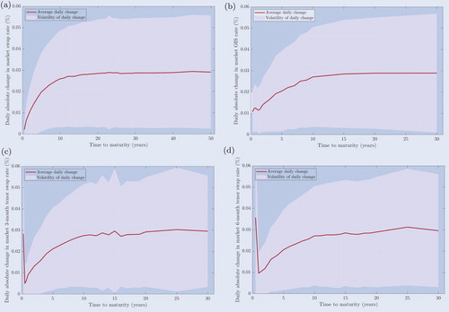
Figure A2. (a) Average daily changes. (b) Volatilities of daily changes. Average daily changes in implied Black volatilities of caps and their volatilities for maturities ranging from 1 year to 20 years and for strike rates ranging from $1.00\mathrm{\%}$ to $10.00\mathrm{\%}$. The daily changes in panel (a) denote averages over the timespan from March 30th, 2012 up until April 28th, 2017. The volatilities in panel (b) represent the standard deviations of these daily changes.

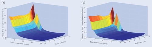
Appendix 4. Additional figures and tables

Figure A3. (a) Single curve - CEV - Deterministic. (b) Multiple curve - CEV - Deterministic. (c) Single curve - DCEV - Deterministic. (d) Multiple curve - DCEV - Deterministic. (e) Single curve - LEV - Deterministic. (f) Multiple curve - LEV - Deterministic. (g) Single curve - QV - Deterministic. (h) Multiple curve - QV - Deterministic. Volatilities of individual caplet prices of each deterministic single and multiple curve model specification for maturities ranging from 1 year to 20 years and for strike rates ranging from $1.00\mathrm{\%}$ to $10.00\mathrm{\%}$. The volatilities are obtained after calibration to the market data on March 30th, 2012 up until March 31st, 2017.

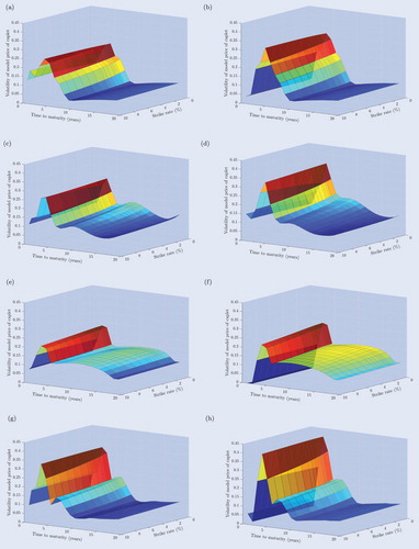
Figure A4. (a) Single curve - LEV - Deterministic. (b) Multiple curve - LEV - Deterministic. (c) Single curve - LEV - Random. (d) Multiple curve - LEV - Random. Volatilities of absolute caplet pricing errors of the single and multiple curve LEV model specifications for maturities ranging from 1 year to 20 years and for strike rates ranging from $1.00\mathrm{\%}$ to $10.00\mathrm{\%}$. The volatilities are expressed in implied Black volatilities and are obtained after calibration to the market data on March 30th, 2012 up until March 31st, 2017.

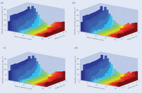
Figure A5. (a) Single curve - CEV - Deterministic. (b) Multiple curve - CEV - Deterministic. (c) Single curve - DCEV - Deterministic. (d) Multiple curve - DCEV - Deterministic. (e) Single curve - LEV - Deterministic. (f) Multiple curve - LEV - Deterministic. (g) Single curve - QV - Deterministic. (h) Multiple curve - QV - Deterministic. Volatilities of out-of-sample caplet prices of each deterministic single and multiple curve model specification for maturities ranging from 1 year to 20 years and for strike rates ranging from $1.00\mathrm{\%}$ to $10.00\mathrm{\%}$. The volatilities are obtained after calibration to the market data on March 31st, 2017 for April 3rd, 2017 up until April 28th, 2017.

References

- Aït-Sahalia, Y. and Lo, A.W., Nonparametric estimation of state-price densities implicit in financial asset prices. J. Financ., 1998, 53, 499–547. doi: 10.1111/0022-1082.215228
- Ametrano, F.M. and Bianchetti, M., Everything you always wanted to know about multiple interest rate curve bootstrapping but were afraid to ask [online]. SSRN.com, 2013. Available online at: https://doi.org/10.2139/ssrn.2219548 (accessed 13 September 2019).
- Amin, K.I. and Morton, A.J., Implied volatility functions in arbitrage-free term structure models. J. Financ. Econ., 1994, 35, 141–180. doi: 10.1016/0304-405X(94)90002-7
- Andersen, L. and Andreasen, J., Volatility skews and extensions of the Libor market model. Appl. Math. Financ., 2000, 7, 1–32. doi: 10.1080/135048600450275
- Andersen, L.B. and Brotherton-Ratcliffe, R., Extended Libor market models with stochastic volatility. J. Comput. Financ., 2005, 9, 1–40. doi: 10.21314/JCF.2005.127
- Bachelier, L., Théorie de la spéculation. Ann. Sci. Éc. Norm. Supér., 1900, 17, 21–86. doi: 10.24033/asens.476
- Barndorff-Nielsen, O.E., Normal inverse Gaussian distributions and the modeling of stock returns. PhD thesis, Department of Theoretical Statistics, University of Aarhus, 1995.
- Barndorff-Nielsen, O.E., Processes of normal inverse Gaussian type. Financ. Stoch., 1997, 2, 41–68. doi: 10.1007/s007800050032
- Beinhofer, M., Eberlein, E., Janssen, A. and Polley, M., Correlations in Lévy interest rate models. Quant. Finance, 2011, 11, 1315–1327. doi: 10.1080/14697688.2010.542299
- Bianchetti, M. and Carlicchi, M., Interest rates after the credit crunch: Multiple-curve vanilla derivatives and SABR [online]. arXiv.org, 2012. Available online at: https://arxiv.org/abs/1103.2567 (accessed 13 September 2019).
- Björk, T., Topics in interest rate theory. In Handbooks in Operations Research and Management Science, edited by J.R. Birge and V. Linetsky, Vol. 15, pp. 377–435, 2007 (Elsevier: Amsterdam).
- Black, F., The pricing of commodity contracts. J. Financ. Econ., 1976, 3, 167–179. doi: 10.1016/0304-405X(76)90024-6
- Black, F. and Scholes, M., The pricing of options and corporate liabilities. J. Polit. Econ., 1973, 81, 637–654. doi: 10.1086/260062
- Brace, A., Ga¸tarek, D. and Musiela, M., The market model of interest rate dynamics. Math. Financ., 1997, 7, 127–155. doi: 10.1111/1467-9965.00028
- Brigo, D. and Mercurio, F., Interest Rate Models—Theory and Practice: With Smile, Inflation and Credit, Springer Finance, 2006 (Springer–Verlag: Berlin, Heidelberg),
- Brigo, D., Mercurio, F. and Morini, M., The LIBOR model dynamics: Approximations, calibration and diagnostics. Eur. J. Oper. Res., 2005, 163, 30–51. doi: 10.1016/j.ejor.2003.12.004
- Cox, J.C., Ingersoll Jr, J.E. and Ross, S.A., A theory of the term structure of interest rates. Econometrica, 1985, 53, 385–407. doi: 10.2307/1911242
- Cox, J.C. and Ross, S.A., The valuation of options for alternative stochastic processes. J. Financ. Econ., 1976, 3, 145–166. doi: 10.1016/0304-405X(76)90023-4
- Cuchiero, C., Fontana, C. and Gnoatto, A., A general HJM framework for multiple yield curve modelling. Financ. Stoch., 2016, 20, 267–320. doi: 10.1007/s00780-016-0291-5
- Cuchiero, C., Fontana, C. and Gnoatto, A., Affine multiple yield curve models. Math. Financ., 2019, 29, 568–611. doi: 10.1111/mafi.12183
- Da Fonseca, J. and Grasselli, M., Riding on the smiles. Quant. Finance, 2011, 11, 1609–1632. doi: 10.1080/14697688.2011.615218
- De Kort, J. and Vellekoop, M., Term structure extrapolation and asymptotic forward rates. Insur. Math. Econ., 2016, 67, 107–119. doi: 10.1016/j.insmatheco.2015.11.001
- Driessen, J., Klaassen, P. and Melenberg, B., The performance of multi-factor term structure models for pricing and hedging caps and swaptions. J. Financ. Quant. Anal., 2003, 38, 635–672. doi: 10.2307/4126735
- Eberlein, E., Eddahbi, M. and Lalaoui Ben Cherif, S.M., Option pricing and sensitivity analysis in the Lévy forward process model. In Innovations in Derivatives Markets: Springer Proceedings in Mathematics & Statistics, edited by K. Glau, Z. Grbac, M. Scherer and R. Zagst, Vol. 165, pp. 285–313, 2016 (Springer: Cham).
- Eberlein, E. and Gerhart, C., A multiple-curve Lévy forward rate model in a two-price economy. Quant. Finance, 2018, 18, 537–561. doi: 10.1080/14697688.2017.1384558
- Eberlein, E., Gerhart, C. and Grbac, Z., Multiple curve Lévy forward price model allowing for negative interest rates. Math. Financ., 2019, 1–29.
- Eberlein, E., Jacod, J. and Raible, S., Lévy term structure models: No-arbitrage and completeness. Financ. Stoch., 2005, 9, 67–88. doi: 10.1007/s00780-004-0138-3
- Eberlein, E. and Kluge, W., Calibration of Lévy term structure models. In Advances in Mathematical Finance: Applied and Numerical Harmonic Analysis, edited by M. Fu, R. Jarrow, J. Yen and R. Elliott, pp. 147–172, 2007 (Birkhäuser: Boston).
- Eberlein, E. and Koval, N., A cross-currency Lévy market model. Quant. Finance, 2006, 6, 465–480. doi: 10.1080/14697680600818791
- Eberlein, E. and Özkan, F., The Lévy LIBOR model. Financ. Stoch., 2005, 9, 327–348. doi: 10.1007/s00780-004-0145-4
- Filipović, D., Term-structure Models: A Graduate Course, Springer Finance, 2009 (Springer–Verlag: Berlin, Heidelberg).
- Fouque, J.P. and Han, C.H., Pricing Asian options with stochastic volatility. Quant. Finance, 2003, 3, 353–362. doi: 10.1088/1469-7688/3/5/301
- García, R.L., Construction and analysis of fixed-income volatility indices. PhD thesis, University of Castile-La Mancha, Ciudad Real, 2013.
- Glau, K., Grbac, Z. and Papapantoleon, A., A unified view of LIBOR models. In Advanced Modelling in Mathematical Finance: Springer Proceedings in Mathematics & Statistics, edited by J. Kallsen and A. Papapantoleon, Vol. 189, pp. 423–452, 2016 (Springer: Cham).
- Grasselli, M. and Miglietta, G., A flexible spot multiple-curve model. Quant. Finance, 2016, 16, 1465–1477. doi: 10.1080/14697688.2015.1108521
- Grbac, Z., Papapantoleon, A., Schoenmakers, J. and Skovmand, D., Affine LIBOR models with multiple curves: Theory, examples and calibration. SIAM J. Financ. Math., 2015, 6, 984–1025. doi: 10.1137/15M1011731
- Grbac, Z. and Runggaldier, W.J., Interest Rate Modeling: Post-crisis Challenges and Approaches, SpringerBriefs in Quantitative Finance, 2015 (Springer: Cham).
- Gupta, A. and Subrahmanyam, M.G., Pricing and hedging interest rate options: Evidence from cap–floor markets. J. Bank Financ., 2005, 29, 701–733. doi: 10.1016/S0378-4266(04)00054-8
- Harms, P., Stefanovits, D., Teichmann, J. and Wüthrich, M.V., Consistent recalibration of yield curve models. Math. Financ., 2018, 28, 757–799. doi: 10.1111/mafi.12159
- Heath, D., Jarrow, R. and Morton, A., Bond pricing and the term structure of interest rates: A new methodology for contingent claims valuation. Econometrica, 1992, 60, 77–105. doi: 10.2307/2951677
- Henrard, M., Swaptions: 1 price, 10 deltas, and ··· 6 1/2 gammas. Wilmott Mag., 2005, 6, 48–57.
- Hilber, N., Reich, N., Schwab, C. and Winter, C., Numerical methods for Lévy processes. Financ. Stoch., 2009, 13, 471–500. doi: 10.1007/s00780-009-0100-5
- Hull, J. and White, A., Pricing interest-rate-derivative securities. Rev. Financ. Stud., 1990, 3, 573–592. doi: 10.1093/rfs/3.4.573
- Jacod, J. and Shiryaev, A.N., Limit Theorems for Stochastic Processes, Grundlehren der mathematischen Wissenschaften, 2003 (Springer–Verlag: Berlin, Heidelberg).
- Jamshidian, F., LIBOR and swap market models and measures. Financ. Stoch., 1997, 1, 293–330. doi: 10.1007/s007800050026
- Joshi, M.S. and Rebonato, R., A displaced-diffusion stochastic volatility LIBOR market model: Motivation, definition and implementation. Quant. Finance, 2003, 3, 458–469. doi: 10.1088/1469-7688/3/6/305
- Kahl, C. and Jäckel, P., Fast strong approximation Monte Carlo schemes for stochastic volatility models. Quant. Finance, 2006, 6, 513–536. doi: 10.1080/14697680600841108
- Kallsen, J. and Shiryaev, A.N., The cumulant process and Esscher's change of measure. Financ. Stoch., 2002, 6, 397–428. doi: 10.1007/s007800200069
- Keller-Ressel, M., Papapantoleon, A. and Teichmann, J., The affine LIBOR models. Math. Financ., 2013, 23, 627–658. doi: 10.1111/j.1467-9965.2012.00531.x
- Kijima, M., Tanaka, K. and Wong, T., A multi-quality model of interest rates. Quant. Finance, 2009, 9, 133–145. doi: 10.1080/14697680802624963
- Kluge, W., Time-inhomogeneous Lévy processes in interest rate and credit risk models. PhD thesis, Albert Ludwig University of Freiburg, Freiburg, 2005.
- Kluge, W. and Papapantoleon, A., On the valuation of compositions in Lévy term structure models. Quant. Finance, 2009, 9, 951–959. doi: 10.1080/14697680902849346
- La Chioma, C. and Piccoli, B., Heath–Jarrow–Morton interest rate dynamics and approximately consistent forward rate curves. Math. Financ., 2007, 17, 427–447. doi: 10.1111/j.1467-9965.2007.00310.x
- Lemke, W., Term Structure Modeling and Estimation in a State Space Framework, Lecture Notes in Economics and Mathematical Systems, 2006 (Springer–Verlag: Berlin, Heidelberg).
- Lopes, S. and Vázquez, C., Real-world scenarios with negative interest rates based on the LIBOR market model. Math. Financ., 2018, 25, 466–482. doi: 10.1080/1350486X.2018.1492348
- Miltersen, K.R., Sandmann, K. and Sondermann, D., Closed form solutions for term structure derivatives with log-normal interest rates. J. Financ., 1997, 52, 409–430. doi: 10.1111/j.1540-6261.1997.tb03823.x
- Morales, M. and Schoutens, W., A risk model driven by Lévy processes. Appl. Stoch. Models Bus. Ind., 2003, 19, 147–167. doi: 10.1002/asmb.492
- Nelson, C.R. and Siegel, A.F., Parsimonious modeling of yield curves. J. Bus., 1987, 60, 473–489. doi: 10.1086/296409
- Raible, S., Lévy processes in finance: Theory, numerics, and empirical facts. PhD thesis, Albert Ludwig University of Freiburg, Freiburg, 2000.
- Rydberg, T.H., The normal inverse Gaussian Lévy process: Simulation and approximation. Commun. Statist. Stoch. Models, 1997, 13, 887–910. doi: 10.1080/15326349708807456
- Sabelli, C., Pioppi, M., Sitzia, L. and Bormetti, G., Multi-curve HJM modelling for risk management. Quant. Finance, 2018, 18, 563–590. doi: 10.1080/14697688.2017.1355104
- Svensson, L.E., Estimating and interpreting forward interest rates: Sweden 1992–1994. Working Paper, University of Stockholm, 1994.
- Vasic˘ek, O., An equilibrium characterization of the term structure. J. Financ. Econ., 1977, 5, 177–188. doi: 10.1016/0304-405X(77)90016-2
- Veronesi, P., Fixed Income Securities: Valuation, Risk and Risk Management, 2010 (John Wiley & Sons, Inc.: Hoboken, NJ).
- Zuhlsdorff, C., The pricing of derivatives on assets with quadratic volatility. Appl. Math. Financ., 2001, 8, 235–262. doi: 10.1080/13504860210127271