
 ?Mathematical formulae have been encoded as MathML and are displayed in this HTML version using MathJax in order to improve their display. Uncheck the box to turn MathJax off. This feature requires Javascript. Click on a formula to zoom.
Abstract
The short-lived arbitrage model has been shown to significantly improve in-sample option pricing fit relative to the Black–Scholes model. Motivated by this model, we imply both volatility and virtual interest rates to adjust minimum variance hedge ratios. Using several error metrics, we find that the hedging model significantly outperforms the traditional delta hedge and a current benchmark hedge based on the practitioner Black–Scholes model. Our applications include hedges of index options, individual stock options and commodity futures options. Hedges on gold and silver are especially sensitive to virtual interest rates.
1. Introduction
Because market participants are generally risk averse, individuals and firms employ hedging strategies that reduce price or return volatility. Investment managers and firm CEO's cannot control various inputs and outputs such as commodity prices, currency prices, equity prices, and bond prices. In such cases, options (and/or futures) are used to take positions that reduce volatility. Options are highly leveraged, have limited liability and are an efficient way to offset, or hedge, this volatility. Thus, there is significant demand for call and put options. In some cases option demand can be satisfied by standardized exchange traded options. In many cases, however, customized options are required and this demand is satisfied by over-the-counter option writers.
The over-the-counter (OTC) market for derivatives is documented by the CitationBank for International Settlements (BIS). According to BIS, the notional amount of outstanding equity linked OTC contracts was 2930 billion US dollars in 2018.Footnote1 The OTC equity options account for more than 60 % of this amount. The outstanding amount of OTC commodity contracts was 1,898 billion US dollars with 7 % of this amount in gold option contracts ($376 billion).
Over-the-counter writers are exposed to risk by virtue of their short positions. To reduce exposure, the writer is obliged to take positions to offset the risk of the written options. By far the most basic and widely used method for reducing this risk is the delta hedge as calculated from the celebrated Black and Scholes (Citation1973) model. The delta hedge can be easily implemented since managing the risk in a portfolio of options involves only trades in the underlying asset and a risk-free account.
Despite its landmark contribution to the financial industry, some Black–Scholes assumptions cannot be empirically justified. Over the past 45 years, researchers have extended or otherwise altered the Black–Scholes model in attempts to improve hedging and pricing. Some models extend the Black–Scholes model to better describe the dynamics of the underlying asset. For example, the jump-diffusion model of stock prices was introduced by Merton (Citation1976) and further extended by a number of authors including Ball and Torous (Citation1985), Naik and Lee (Citation1990), and Bates (Citation1991). Hull and White (Citation1987, Citation1988), and Heston (Citation1993) were early proponents of models that include both the underlying and stochastic volatility as state variables. Bates (Citation1996), and Duffie et al. (Citation2000) develop models that includes both jumps and stochastic volatility. In a landmark study, Bakshi et al. (Citation1997) investigated several models and hedging techniques.
Theoretical models that effectively hedge jump-diffusions require the addition of options to the short-term portfolio. See, for example, Andersen and Andreasen (Citation2000) or He et al. (Citation2006). In addition, models with multiple hedging instruments also theoretically improve hedging performance for smooth diffusions. In practice, however, multiple instruments pose significant issues. For example, a hedge portfolio with the underlying and an option would be efficacious only if there were synchronous or near synchronous trades of the target (hedged) option, the underlying, and the hedging option(s). Since options are typically less liquid than the underlying, synchronicity is a significant problem. Because of these difficulties and other considerations such as transaction costs, the single instrument hedge using the underlying remains the preferred approach among practitioners.
Notwithstanding improvements in modeling prices, the workhorse for pricing and single instrument hedging is the Practitioner Black–Scholes model. A key element of this model is a volatility surface that is derived by fitting implied volatilities to moneyness and maturity (Christoffersen and Jacobs Citation2004). Other approaches have been developed to improve hedging performance by adjusting the Black–Scholes delta. One alternative that has found traction in the literature is the minimum variance (MV) hedge ratio. The MV hedge remedies the failure of the delta hedge to account for multiple state variables that are correlated with the underlying. Shortcomings of the delta hedge have been addressed by a number of authors including Hagan et al. (Citation2002), Bartlett (Citation2006), Alexander and Nogueira (Citation2007), and Hull and White (Citation2017). Other considerations also favor the MV hedge over the delta hedge. Christoffersen and Jacobs (Citation2004) provide a compelling argument for choosing a hedging loss function that is consistent with the parameter estimation loss function. In its simplest incarnation, this means that a least squares loss function should be used to evaluate hedging performance if parameters are chosen to minimize in-sample squared errors.
Minimum-variance deltas have been developed using stochastic volatility as an additional state variable. Hull and White (Citation2017) document that a number of researchers have shown improved hedging performance by combining the Practitioner Black–Scholes delta and Practitioner Black–Scholes vega. In these models, ‘Practitioner’ implies that a formal stochastic process is not assumed but implied from the data. Hull and White develop a model of this nature by empirically determining the partial derivative of expected volatility with respect to price (vega). The model is tested against the SABR stochastic volatility model (Hagan et al. Citation2002) and the local volatility model using data from widely traded stocks, commodities, and ETFs. Their primary focus is hedging options on the S&P 500 index. According to their performance metric (‘gain’), the HW hedging model shows significant improvements over the SABR model and the local volatility model. The HW hedge performance was better for calls than puts and better for indices than individual stocks.
We develop a different MV hedge based on a practitioner version of the short-lived arbitrage (SLA) model of Otto (Citation2000). The formula for the SLA model is essentially the same as that of the Merton Stochastic Interest Rate model. However, it differs in one crucial aspect. The short-lived arbitrage is latent but expressed as a state variable in the Merton bond price term. Since it is unobservable, Otto refers to the Merton bond term as a ‘virtual bond.’ Hilliard and Hilliard (HH, Citation2017), extend the Otto model for correlations with the underlying and find that jointly implied volatility and virtual bond price significantly improves fit vis-á-vis the Black–Scholes pricing model with implied volatility. They also find that put options have higher prices than call options relative to their Black–Scholes counterparts, consistent with the empirical findings of Cremers and Weinbaum (Citation2010). Motivated by significantly better in-sample fit, we use the SLA model to develop a MV hedge ratio using jointly implied volatility and virtual bond price that takes delta, vega, gamma and rho exposure into consideration. Consistent with the SLA model, Greeks are computed using implied yield-to-maturity rather than observed rates.
Using an extensive dataset from selected indices, individual stocks, and commodities, we demonstrate that SLA hedge ratios produce MV hedges that dominate delta hedges and our benchmark, the Hull and White (Citation2017) hedge. In particular, compared to alternative hedges, the SLA hedge significantly reduces mean absolute errors, standard deviations, and the RMSE of daily hedging errors. In terms of point estimates, error metrics for stock indices from the SLA hedge were less than those of alternative hedging methods for calls in 36 out of 36 metrics. For puts, error metrics for the SLA hedge were better in 34 of 36 cases. Results were essentially the same for stocks and commodities. We use the Diebold-Marino statistic to test for significance between the SLA hedge and alternatives hedges. Counts of significance for the SLA hedge versus alternatives at the 0.01 or 0.05 level for calls were as follows: 29 of 36 (indices), 22 of 36 (stocks), and 22 of 36 (commodities). For puts, the corresponding counts were: 18 of 36 (indices), 7 of 36 (stocks) and 26 of 36 (commodities). There were no cases where an alternative hedge was significantly better than the SLA hedge.
We decomposed the MV hedge ratio into component parts corresponding to the Greeks. The composition of the ratios was similar for both puts and calls. The BS delta terms contributed about 85 % to the MV hedge ratio for equity indices and stocks and about 60 % to the hedge ratio for commodities. The vega ( term contributed about 20 % to the crude oil hedge ratio. For calls, rho
contributed about 15 % to gold and silver hedge ratios, consistent with evidence that precious metal returns are correlated with interest rates. This supports Bailey (Citation1987) who used the Ramaswamy and Sundaresen (Citation1985) stochastic interest model to study Gold Comex Options. He found average errors of $43 per contract with a stochastic interest rate model while a constant interest rate model had average errors of $96 dollars per contract.
2. Minimum variance hedging
Under the classical Black–Scholes model, the underlying asset follows a geometric Brownian motion (gBm) with constant drift and volatility. By construction, the delta of a call (
) nulls out random effects in a portfolio consisting of a call and the underlying asset.
Equivalently, delta minimizes the variance of an investment portfolio consisting of an option, stock and bond written as
(1)
(1) where C is a call, S is the underlying spot price, B is a risk-free bond, and δ is the hedging ratio. The local change is
with variance
The first-order condition for minimum variance (
leads to the result that
so that the minimum variance delta,
is equal to the standard Black–Scholes delta,
when the only state variable is the underlying.
2.1. Minimum-Variance hedge ratios under multiple state variables
Consider an option pricing model based on diffusions in the underlying, volatility and interest rates. Denote the equilibrium (call) option price as with local change
Using the same setup as in equation (Equation1
(1)
(1) ), the minimum variance hedge ratio
can be expressed as
(2)
(2) The easy result is that
when covariances are zero but otherwise
depends on covariances, vega
and rho (
But the result is not without complications. Specifically, how do we compute the partials? Do we require the multi-state equilibrium model or will Black–Scholes partials suffice? The answer to the latter question is a qualified yes. Bates (Citation2005) and Alexander and Nogueira (Citation2007) note that a sufficient condition for model free hedge ratios for options is that the underlying process be scale invariant. This condition is satisfied by most option pricing models, with notable exceptions being models based on arithmetic Brownian motion or the CEV model. When the underlying is scale independent, pure vanilla options are homogeneous of degree one (Merton Citation1973) and a well known result of Euler gives
(3)
(3) The notion that delta (
) is model independent follows from the fact that, if traded, C is observable and
can be estimated from a set of prices with different strikes. Ergo, the delta is model independent. Similar model independence can be inferred for gamma (
). See Bates (Citation2005).
Alexander and Nogueira (Citation2007) state that if competing models are scale invariant ‘the only reason their price ratios differ is because they have a different fit to the market prices of options.’ In fact, BS hedge ratios can be quite different from those of smile-consistent models. The good news is that for the data studied, AN report that BS delta and gamma hedges perform better than model independent hedges for equity index options. We assume that MV approximations in equation (Equation2(2)
(2) ) are useful even when Greeks from multi-state equilibrium models are replaced by BS Greeks. And, in any case, we test their efficacy against alternatives on a database of heavily traded indices, stocks and commodities.
There is also a growing literature on how MV hedge ratios can be obtained by adjusting BS deltas. As noted by AN and outlined in equation (Equation2(2)
(2) ), the adjustment depends on local covariances between the underlying and the additional state variables. Adjustments have been investigated by Hull and White (Citation2017), Engelmann et al. (Citation2006) and Alexander and Kaeck (Citation2012). Alexander and Kaeck use the chain rule to compute the smile adjustment
. The covariance adjustment and smile adjustment are approximately the same since
implies
and thus
. The Alexander and Kaeck result can be obtained for three state variables by a straightforward extension of the chain rule. In the HW model,
is approximated by
where
is implied volatility.
2.2. The model of short-lived arbitrage
An important component of our hedging approach are the comparative statics suggested by a short-lived arbitrage model that depends on the value of a virtual bond. The Black–Scholes model is based on number of perfect capital market assumptions and fundamentally on the assumption of the absence of arbitrage. However, empirical studies have documented short-lived arbitrage opportunities in otherwise well functioning markets. See Sofianos (Citation1993), HH and others. In a world of rational economic agents, the existence of arbitrageurs is prima facia evidence of arbitrage opportunities.
Otto's proxy for (latent) short-lived arbitrage is an Ornstein-Uhlenbeck process of the form
(4)
(4) that is pinned to zero at option expiration (T) and with long-term mean
. The arbitrage variable is thus a bridge between current value
and
. Using conditional probabilities, HH convert the OU diffusion to a bridge diffusion and extend the Otto model to account for correlations between the arbitrage and underlying diffusion.
Assuming gBm for the underlying and using the Garman (Citation1977) setup for pricing with multiple state variables, the instantaneous change in the candidate portfolio sans delta risk is set equal to , where r is the risk-free rate. Although cast as a short-lived-arbitrage model, the variable
proxies for net frictions that act to perturb the risk-free rate. The net result is a pricing model that is isomorphic to Merton's stochastic interest rate model (
is the instantaneous virtual rate) where the bond is a non-traded ‘virtual bond.’ The virtual bond is of the form
where
is the risk-free bond and
is a function of the parameters of the bridge diffusion. For the functional form of V
see Otto or HH.
The SLA model for a call option is written
(5)
(5) where S is the underlying spot price, K is the strike price,
is the virtual bond and R is the virtual yield. The arguments
and
are standard BS calculations when volatilities and yields are implied. The pertubation from the constant rate may be because of short lived arbitrage, market frictions, or stochastic interest rates. It is not the same as a pure stochastic interest rate model, however, since the stochastic interest rate is the same for all firms in the economy while the virtual yield is unique to the frictions on the equity of a firm. For margined options, greek formulas do not depend on the risk-free rate.Footnote2 For these options, the perturbed rate is
the virtual bond is,
and
is the pertubation due to frictions net of interest rates.
Jointly implying volatility and the virtual bond, HH find that the SLA model significantly improves in-sample fits relative to the Black–Scholes model for each of a select set of stocks. Better SLA pricing performance suggests that ‘practitioner’ SLA-based hedges may also perform better. And this means specifically that implying latent virtual yields might lead to improved hedges. For more detail on the issue of hedging and model fit see Alexander and Kaeck (Citation2012).
2.3. Practitioner short-lived arbitrage dynamics
We consider non-local time and the role of gamma in developing the SLA hedge ratio. Local terms are replaced by finite terms
and changes in
are written
(6)
(6) and so
(7)
(7) Assuming
is normal with mean
and variance
,
and the minimum variance hedge ratio is
(8)
(8) where
and
. After σ and R are jointly implied using the SLA model, we compute Greeks and use equation (Equation8
(8)
(8) ) in a regression setup to estimate coefficients
and
2.4. Data
We test the proposed hedging method for options on selected indices, individual stocks, and commodity futures. The indices are the S&P 500 (SPX), the Nasdaq 100 (NDX), and the Russell 2000 (RUT); the individual stocks are Amazon (AMZN), GoogleFootnote3 (GOOGL), and Berkshire Hathaway (BRK.A); the three commodity futures are Brent Crude Oil Futures, 100 oz Gold Futures, and 5000 oz Silver Futures. These assets and contracts are highly liquid and have been widely studied in the financial economics literature. We obtain daily interest rates, equity prices, and option data from OptionMetrics. Dividend yields on the underlying indices are from FactSet. The data for the commodity futures are from The Intercontinental Exchange (Citation2017). The options on indices are European style while options on individual stocks and commodities are American style. Options on Brent Crude futures are margined style and have no early-exercise premiums under weak assumptions (Hilliard and Hilliard Citation2019). The options on commodities from the ICE do not contain information on Greeks and so the test design is slightly different from the test design for options on indices and individual stocks. Except for Gold and Silver, the data is from the period 2 January 2013 through 27 June 2019. Data for options on 100 oz Gold Futures and 5000 oz Silver Futures was first available on 2 January 2014.
For options on indices and individual stocks, we retain only those with available bid price, offer price, implied volatility, delta, gamma, vega, and theta. We also delete options with no volume, except for options on Gold and Silver since available data does not report volume. To evaluate daily hedging performance, we select options that have at least two successive trading days. Options are retained if the maturity is at least 14 calendar days and the average of best bid price and best offer price is at least 25 cents. To avoid deep in- and out-of-the-money options, we delete call options with delta less than 0.05 or greater than 0.95 and put options with delta less than −0.95 or greater than −0.05.
We summarize the data for indices, individual stocks, and commodities in tables –. In table we present summary statistics for options on indices. More puts are traded than calls and short-term options dominate long-term options. There are 443,168 observations on S&P 500 call options and 800,210 observations on S&P 500 put options. The average price of call options is higher than the average price for put options for all indices.
Table 1. Summary statistics for index options.
For individual stocks shown in table , there are more call contracts traded than put contracts. And there are more contracts on Amazon options than on Google or Berkshire Hathaway. Options on individual stocks also tend to have longer maturities. The average maturities for calls on the S&P 500, the NASDAQ 100 and the Russell 2000 are, respectively 51, 47, and 48 days while average maturities on Amazon, Google and Berkshire Hathaway are, respectively, 121, 111, and 198 days. Longer maturities and the reversal in contract volume is consistent with the notion that there is more hedging activity in indices and speculative activity in individual stocks.
Table 2. Summary statistics for options on selected stocks.
Descriptive statistics for options on commodity futures are given in table . Statistics for crude oil are based on the number of actual trades. Unfortunately, the ICE does not report volume on Gold and Silver so statistics here are derived from all open contracts. Summary statistics for the underlying commodity futures are given in table .
Table 3. Summary statistics on options on commodity futures.
Table 4. Summary statistics on commodity futures.
3. Hedge ratio estimation and error metrics
Estimating the MV delta for the Short Lived Arbitrage (SLA) model and testing for errors is done in several steps:
Estimate implied parameters. Using daily data we jointly estimate implied volatility and virtual yield for each day
. All observations surviving screens are used to calculate the
Compute Greeks. Use the parameters implied in step 1. and the SLA model to compute Greeks delta
OLS regressions. Using 26 weeks of data, OLS regressions are used to estimate β coefficients required for the MV delta. We estimate
Compute hedge ratios. Using
Compute errors. For each option (i) and for each of the five ratios
Error Metrics. Using errors computed in step 5. we use all observations and compute mean absolute errors, the standard deviations of errors, and the root-mean-square of errors (RMSE). We focus more on RMSE errors because (1) Christoffersen and Jacobs (Citation2004) persuasively argue that the loss function should be the same as the loss function used to estimate parameters and (2) it is a measure of fit commonly used by other researchers. Results from the standard deviation metric are included but they are almost the same as RMSE results (they are mathematically the same if the sample mean is zero). We include the absolute error metric.
Significance Tests. The Diebold and Mariano (Citation1995) setup for a sequence of prediction errors is a follows: Let
4. Results
We use several error metrics to compare hedging results using the BS delta, the HW delta, and the SLA delta. The BS delta is the Greek delta while the HW delta and SLA delta are minimum variance approximations. Hedge ratios are designated by: (BS hedge),
(HW hedge), and
(SLA hedge). Greeks for the BS delta and HW deltas are computed using both observed and implied interest rates. Greeks for the SLA hedge are computed using implied yields.
4.1. Point estimates
As precursor to detailed significance tests, we first present a general overview of hedging error metrics for options on the S&P 500 index for different delta buckets in figures one through four.Footnote6 There are 10 buckets containing observations for call deltas between 0.05 and The 0.1 bucket consists of deltas between 0.05 and 0.15. Other buckets are similarly centered. Error metrics are normalized by the average price of options in the bucket. Put buckets are similarly defined with negative deltas.
Mean absolute value errors for calls are shown in figure . The error metric for the hedge is smaller than the corresponding metric for the
hedge for all delta buckets with near equality for the 0.2 bucket. The error metric for
hedge is larger than that of the
hedge for all buckets and also larger than that of the
hedge except for the largest four buckets (0.6, 0.7,
and 0.9).
Figure 1. SPX Absolute Value Hedging Error for Calls by Delta Category. Mean Absolute Errors normalized by average call price. Hedge ratios are set by the Black–Scholes delta (), Hull-White Minimum Variance delta (
) and Short-Lived Arbitrage Model delta (
). For data description see notes, table .
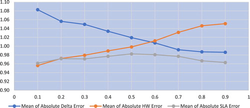
Table 5. Error metrics and significance tests for calls on indices.
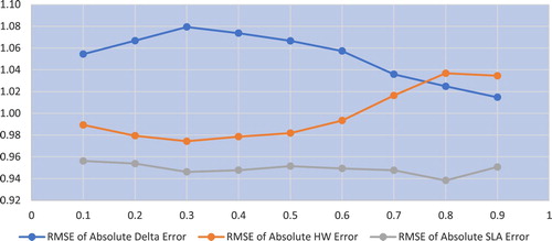
RMSE errors for calls are shown in figure . Results are similar to those of the absolute value metric. The error metric for the hedge is smaller than those of other hedges for all buckets. Similar to figure ,
and
hedges strictly dominate the
hedge with the exception of the metric for buckets 0.8 and 0.9 where the
hedge metric is better than the
metric.
Figure 2. SPX RMSE Hedging Errors for Calls by Delta Category. RMSE Errors normalized by average call price. See notes in figure .
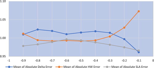
Mean absolute errors for puts are shown in figure . The error metric for the hedge is less than that of the
for all buckets except the
bucket and less than that of the
hedge for all buckets except for the
and
bucket where the difference is negligible.
Figure 3. SPX Absolute Value Hedging Error for Puts by Delta Category. Mean Absolute Errors normalized by average put price. See notes figure .
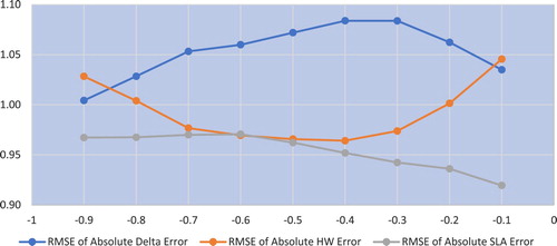
RMSE errors for puts are shown in figure . The hedge has lower metrics than the
and the
for all buckets except equality with
at the
bucket.
Figure 4. SPX RMSE Hedging Errors for Puts by Delta Category. RMSE Errors normalized by average put price. See notes in figure .
4.2. Diebold-marino test statistics
In tables – we present error metrics for hedging calls on selected indices, stocks, and commodities. In these tables we consider five different hedging ratios: The Black–Scholes delta with observed interest rates the Black–Scholes delta with implied interest rates
the Hull-White minimum variance delta with observed interest rates
, the Hull-White minimum variance delta with implied interest rates
and the Short-Lived-Arbitrage minimum variance delta
All ratios with implied interest rates are jointly implied with volatility.
Table 6. Error metrics and significance tests for calls on stocks.
Table 7. Error metrics and significance tests for calls on commodities.
We use the Diebold-Marino statistic (see Section 3) to test for significant differences between error metrics. The difference in error metrics is computed by subtracting the sample mean of the error metric from that of the candidate error metrics. A positive DM statistic corresponds to a smaller
hedging error.
4.2.1. Results for hedging calls on indices
Results for hedging calls on the S&P 500, Russell 2000 and NASDAQ indices are given in table . We focus our discussion on RMSE errors but results are similar for standard deviations and for absolute errors. Panel A gives results for the S&P 500. The hedge gives the smallest RMSE and is significantly less than other hedges by the DM test on 12 of 12 comparisons. Panel B in table shows similar but somewhat weaker results for the Russell 2000. RMSE errors for the
hedge are all smaller and differences are significant at the 0.01 or 0.05 for 9 of 12 comparisons. NASDAQ results are given in panel C. Tests statistics are positive for all metrics and significant for the RMSE metric versus all alternatives.
4.2.2. Results for hedging calls on stocks
Results for hedging calls on Amazon, Google and Berkshire stocks are given in table . With one exception, the DM test statistics for the absolute value, standard deviation, and RMSE metrics are all positive, indicating lower average errors for the hedge. The results for Berkshire, panel C, are strongest. The
error metric is significant at the 0.05 level for all DM statistics and at the 0.01 level for nine DM statistics.
4.2.3. Results for hedging calls on commodities
Results for oil, gold, and silver call options are given in table . The DM test statistic is positive for all metrics and all commodities. For gold and silver, the DM statistic is significant at 0.01 or 0.05 in 9 of 12 comparisons. The results are weakest for oil, where the DM test statistic is positive and significant at the 0.05 level in 4 of 12 cases. Compared to gold and silver, oil is a bit different since it has stochastic convenience yield while silver and especially gold are generally considered investment assets. Thus a Black–Scholes type model is more appropriate for gold and silver than for oil.
4.2.4. Hedging gains for calls
As in Hull and White (Citation2017), we construct a measure of the improvement of the hedge using the hedge as the benchmark. The measure is computed as
(13)
(13) The error metrics are average absolute error, standard deviation, and RMSE. Comparison hedges use the two
ratios and the two
ratios. A gain greater than one corresponds to a smaller error metric using the
hedge ratio. Results are given in table . Gains are greater than one for all indices, stocks, and commodities. The greatest RMSE gain is versus Berkshire Hathaway and
hedge (
). The smallest RMSE gain is versus Amazon and the
hedge (
). The
hedge versus crude oil and gold was uniformly large versus all alternative hedging methods. The smallest RMSE gains were against indices, stocks and the
hedge ratio.
Table 8. Gain in squared error metric ratios for calls using SLA.
4.2.5. Results for put hedges
Tables – give results for put hedges. Overall, the results for hedging puts on indices, table , are similar to the results for calls with the hedge having a positive DM statistics in every comparison except one. Counts and significance levels for the S&P 500 and NASDAQ were relatively weaker however. Significance counts at 0.01 or 0.05 were: S&P 500 (6 of 12), Russell 2000 (9 of 12) and NASDAQ (3 of 12). While DM t-statistics were positive, the
hedge was not significantly better than the
hedge for the S&P 500 and NASDAQ.
Table 9. Error metrics and significance tests for puts on indices.
Table 10. Error metrics and significance tests for puts on stocks.
Table 11. Error metrics and significance tests for puts on commodities.
The results for puts on stocks, table , were also weaker than the results for calls. While positive, DM statistics were not significant at 0.01 or 0.05 for Amazon and in only two cases for Google. Anomalous to all other results, the DM statistic for the RMSE metric versus the hedge was negative albeit not significant for Amazon.
Results for hedging puts on commodities were strong (table ). All DM-statistics were positive and significant at the 0.01 or the 0.05 level in 26 of 36 cases. But, similar to calls, t-stats for put hedges were weaker for oil than for gold and silver.
Gain results for puts are given in table . Gains for commodities were all greater than one and generally larger than gains for stocks. Gains are also greater than one for all indices with the exception of the absolute error metric and and
hedges for NASDAQ. All gains are greater than one for Amazon and Berkshire but less than one for the absolute error metric for Google and the
and
hedges. In summary, gains are positive in 32 of 36 cases.
Table 12. Gain in squared error metric ratios for puts using SLA.
4.3. Parameters and hedging coefficients
Hedging improvements are a result of using implied interest rates and adding greeks beyond the Black–Scholes delta. Percentage contributions to the average SLA hedge ratios are depicted in figures and . For calls, figure , the Black–Scholes delta term contributes about 80 % to the ratio for indices and 85 % for stocks. Vega and gamma terms contribute slightly more than the rho term. But commodities are different. For hedge ratios on oil, the average contribution of the delta term falls to about 55 % while vega contribution increases to about 25 %. Rho and gamma each contribute about 10 %. For gold and silver, the delta contribution increases to about 65 % while rho increases to about 15 %. The combined contribution of vega and gamma is about 20 %.
Figure 5. Average contribution of Greek terms to SLA hedge ratio for calls. See notes, table .
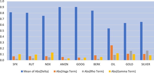
Figure 6. Average contribution of Greek terms to SLA hedge ratio for puts. See notes, table .
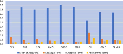
The pattern of greek contributions to hedge ratios for puts shown in figure is similar to that of calls for indices and stocks. However, rho is less heavily weighted for silver and gold, contributing just over 5 % to the hedge ratio.
The importance of rho, for hedging gold and silver calls and puts contrasts with its negligible contribution to the hedge ratio for indices and stocks. This is consistent with evidence that precious metal returns are correlated with interest rates. Precious metals, especially gold, are used as effective hedges against inflation and economic uncertainty. In addition gold is denominated in US dollars in international markets and is influenced by U.S. interest rate policies (Wang and Ling Chueh Citation2013). Thus, stochastic interest rates are likely an important state variable in equilibrium option pricing models for gold and silver. In a study of Gold Comex Futures Options, Bailey (Citation1987) found that the Ramaswamy and Sundaresen (Citation1985) stochastic interest rate model had an average error of $43 per contract while a constant interest rate model had an error of $96 dollars per contract.
5. Robustness
The effect of the length of the hedging horizon and level of volatility warrant further investigation. We extended the hedging horizon from 5 to 20 days and examined equity (oil) hedges in periods of extreme volatility 1 January 2007 to 31 December (1 September 2008 to 31 December 2010). Because of data limitations and for economy of presentation, we look at subsets of scenarios examined in earlier sections.
5.1. Extended hedging horizon
Using the same setup as before, we examined hedges with horizons of 5, 10, and 20 days for puts and calls. We only compute RMSE errors for HW and SLA hedges. The results are shown in table . For indices (Panel A), there is virtually no change in RMSE as the horizon is extended. For Amazon, the daily RMSEs over 5, 10, and 15 day horizons are 2.7453, 2.7577 and 2.7470. The HW hedge has a smaller RMSE than the SLA hedge at only one of 18 data points (the 20 day horizon for the Russell 2000).
Table 13. Extended horizon RMSE results: comparison of Hull–White MV ratios and short-lived-arbitrage MV ratios.
Results for stocks are shown in Panel B. The RMSEs for all SLA hedges are smaller than the HW RMSEs for puts and calls at all horizons. The horizon effect is negligible. At first blush it seems curious that Berkshire Hathaway RMSEs are about are 1/4 and 1/10 those of Google and Amazon, respectively. But from table , average Berkshire Hathaway option prices follow approximately the same ratio.
Commodity results are shown in Panel C. Increases in RMSEs are usually found only in the third significant place. In fact, for silver and gold there is no difference over horizons until the fifth or sixth place (not shown). Point estimates of SLA RMSEs are smaller than HW RMSEs in every case.
5.2. Volatility effects
Our initial focus was on data from 2 January 2013 to 27 June 2019 (benchmark period). Here we investigate hedging performance during the high volatility period from 1 January 2006 through 31 December 2010. This period includes the subprime crisis and recession dated from December 2007 to June 2009. We do not have options data for silver and gold during this period (trades on ICE began in 2014) and to keep the number of tables manageable we only investigate the S&P 500, Amazon and Brent Crude.
Results for calls are shown in table . The differences in the magnitude of errors and DM statistics in the volatile versus the benchmark period are small and follow no systematic pattern. RMSEs for the SLA hedge and the benchmark (volatile) period are: S&P 500 2.0269 (1.6792), Google 1.0941 (1.3570) and Brent Crude 0.1169 (0.2096). The SLA hedge still dominates alternatives in the volatile period. All DM statistics are positive and are significant at 0.01 or 0.05 as follows: S&P 500 (12 of 12), Google (2 of 12) and Brent Crude Oil (6 of 12).
Table 14. Error metrics and significance tests for calls during high volatility.
Results for puts are shown in table . RMSEs are: Benchmark (volatile) period: Brent Crude 0.1152, (0.1623), S&P 500 2.7453, (1.7338) and Google 1.2814, (1.2412). All DM statistics are positive and DM statistics are significant at 0.01 or 0.05 as follows: S&P 500 (10 of 12), Google (0 of 12), and Brent Crude Oil (2 of 12). Results are a bit weaker for puts compared to those in the benchmark period.
Table 15. Error metrics and significance tests for puts during high volatility.
In summary, the SLA hedge performed well for calls in periods of high volatility. It does less well for puts though DM statistics remain positive for all cases. Only Brent Crude RMSE errors were larger for both put and calls during the volatile period.
6. Conclusions
Motivated by its derivation, the original benchmark for hedging custom option positions is the Black–Scholes delta. Based on least square loss functions, numerous authors have proposed choosing hedge ratios based on least squares approximations. These ratios depend on the pricing model used and the type of approximation employed. We develop a ratio based on a so-called ‘short lived arbitrage’ model. In this model, the interest rate is latent and embodies deviations from model assumptions such as the possibility of arbitrage. We refer to this rate as the virtual interest rate. As such, we imply interest rates in the same manner that volatilities are implied. Using a least squares formulation we develop a ratio that is a function of the greeks delta, vega, rho, and gamma. The greeks are computed using the implied interest rate.
Using a large data set that includes more than 7 years of data and up to 800 000 observations, we evaluate the performance of the SLA hedge on a set of indices, stocks and commodities. We evaluate performance using the absolute value, standard deviation, and RMSE error metrics. In terms of point estimates, error metrics from the SLA hedge bests alternatives for calls on indices in 36 of 36 metrics. For puts, error metrics from the SLA hedge was better in 34 of 36 cases.
We use the Diebold-Marino statistic to test for significance between the SLA hedge and alternative hedges. Counts of significance at the 0.01 or 0.05 level for calls were as follows: 29 of 36 (indices), 22 of 36 (stocks), and 22 of 36 (commodities). For puts the corresponding counts are: 18 of 36 (indices), 7 of 36 (stocks) and 26 of 36 (commodities). Results were generally robust to periods of market stress and extended hedging horizons.
The SLA hedge ratios were composed of four greeks. For calls, delta makes the strongest contribution, averaging about 85 % of the hedge ratio for indices and stocks. The contributions to the hedge ratio for commodity hedges is a bit different. Delta accounted for about 55 % of the SLA hedge and rho up to 15 %. Contrasted to its role in hedging indices and stocks, rho was especially important in gold and silver hedges, perhaps due to the strong relationship between precious metals and interest rates.
The main contribution of the paper is the novel use of the virtual interest rate. Due to violations of standard pricing assumptions, the virtual interest rates is in effect a pertubation of the observed interest rate. We find that the perturbed rate can be used to improve hedge ratios in a practitioner Black–Scholes model.
Disclosure statement
No potential conflict of interest was reported by the author(s).
Notes
2 The Brent Crude oil options that we use are margined options.
3 Google essentially renamed itself as ‘Alphabet’ in August 2015. It continues to trade under the same GOOG symbol.
4 The dataset contains 338 observation weeks for indices, stocks and oil. There are 286 observation weeks for gold and silver.
5 We use the Dmarino module in Stata and Bartlett HAC standard errors to compute t-statistics (Baum Citation2011).
6 The delta bucket is defined as the usual Black–Scholes delta.adjusted for dividends.
References
- The Intercontinental Exchange, 2017, www.theice.com/products/219/Brent-Crude-Futures.
- Bank for International Settlements, https://stats.bis.org/statx/srs/table/d8?p=20182&c=#.
- Alexander, C. and Kaeck, A., Does model fit matter for hedging? Evidence from FTSE 100 options. J. Futures Mark., 2012, 32, 609–638. doi: 10.1002/fut.20537
- Alexander, C. and Nogueira, L.M., Model-free hedge ratios and scale-invariant models. J. Bank. Financ., 2007, 31, 1839–1861. doi: 10.1016/j.jbankfin.2006.11.011
- Andersen, L. and Andreasen, J., Jump-diffusion processes: Volatility smile fitting and numerical methods for option pricing. Rev. Deriv. Res., 2000, 4, 231–262. doi: 10.1023/A:1011354913068
- Bailey, W., An empirical investigation of the market for comex gold futures options. J. Financ., 1987, 42, 1187–1194. doi: 10.1111/j.1540-6261.1987.tb04360.x
- Bakshi, G., Cao, C. and Chen, Z., Empirical performance of alternative option pricing models. J. Financ., 1997, 52, 2003–2049. doi: 10.1111/j.1540-6261.1997.tb02749.x
- Ball, C.A. and Torous, W.N., On jumps in common stock prices and their impact on call option pricing. J. Financ., 1985, 40, 155–173. doi: 10.1111/j.1540-6261.1985.tb04942.x
- Bartlett, B., Hedging under SABR Model, Wilmott Magazine, July-August, 2–4, 2006.
- Bates, D.S., The crash of '87. Was it expected? The evidence from options markets. J. Financ., 1991, 46, 1009–1044. doi: 10.1111/j.1540-6261.1991.tb03775.x
- Bates, D.S., Jumps and stochastic volatility: Exchange rate processes implicit in deutsche mark options. Rev. Financ. Stud., 1996, 9, 69–107. doi: 10.1093/rfs/9.1.69
- Bates, D.S., Hedging the smirk. Financ. Res. Lett., 2005, 2, 195–200. doi: 10.1016/j.frl.2005.08.004
- Baum, C.F., DMARIANO: Stata module to calculate Diebold-Mariano comparison of forecast accuracy. Statistical Software Components S433001, Boston College Department of Economics, revised 26 Apr 2011, 2011.
- Black, F. and Scholes, M., The pricing of options and corporate liabilities. J. Polit. Econ., 1973, 81, 637–654. doi: 10.1086/260062
- Christoffersen, P. and Jacobs, K., The importance of the loss function in option valuation. J. Financ. Econ., 2004, 7, 291–318. doi: 10.1016/j.jfineco.2003.02.001
- Cremers, M. and Weinbaum, D., Deviations from put-call parity and stock return predictability. J. Financ. Quant. Anal., 2010, 45, 335–367. doi: 10.1017/S002210901000013X
- Diebold, F.X. and Mariano, R.S., Comparing predictive accuracy. J. Bus. Econ. Stat., 1995, 13, 252–263.
- Duffie, D., Pan, J. and Singleton, K., Transform analysis and asset pricing for affine jump-diffusions. Econometrica, 2000, 68, 1343–1376. doi: 10.1111/1468-0262.00164
- Engelmann, B., Fengler, M.R. and Schwendner, P., Hedging under alternative stickiness assumptions: An empirical analysis for barrier options. J. Risk, 2006, 12, 53–77. doi: 10.21314/JOR.2009.199
- Garman, M.B., A general theory of asset valuation under diffusion state processes. No. 50, Research Program in Finance Working Papers, University of California at Berkeley, 1977.
- Hagan, P., Kumar, D., Lesniewski, A. and Woodward, D., Managing smile risk. Wilmott Mag., 2002, 1, 84–108.
- He, C., Kennedy, J.S., Coleman, T.F., Forsyth, P.A., Li, Y. and Vetzal, K.R., Calibration and hedging under jump-diffusion. Rev. Deriv. Res., 2006, 9, 1–35. doi: 10.1007/s11147-006-9003-1
- Heston, S.L., A closed-form solution for options with stochastic volatility with applications to bond and currency options. Rev. Financ. Stud., 1993, 6, 3327–343. doi: 10.1093/rfs/6.2.327
- Hilliard, J.E. and Hilliard, J., Option pricing under short-lived arbitrage: Theory and tests. Quant. Finance, 2017, 17, 1661–1681. doi: 10.1080/14697688.2017.1301677
- Hilliard, J.E. and Hilliard, J., A jump-diffusion model for pricing and hedging with margined options: An application to Brent crude oil contracts. J. Bank. Financ., 2019, 98, 137–155. doi: 10.1016/j.jbankfin.2018.10.013
- Hull, J. and White, A., The pricing of options on assets with stochastic volatilities. J. Financ., 1987, 42, 281–300. doi: 10.1111/j.1540-6261.1987.tb02568.x
- Hull, J. and White, A., The use of the control variate technique in option pricing. J. Financ. Quant. Anal., 1988, 23, 237–251. doi: 10.2307/2331065
- Hull, J. and White, A., Optimal delta hedging for options. J. Bank. Financ., 2017, 82, 180–190. doi: 10.1016/j.jbankfin.2017.05.006
- Merton, R., Theory of rational option pricing. Bell J. Econ. Manage. Sci., 1973, 4, 141–183. doi: 10.2307/3003143
- Merton, R., Option pricing when underlying stock returns are discontinuous. J. Financ. Econ., 1976, 3, 125–144. doi: 10.1016/0304-405X(76)90022-2
- Naik, V. and Lee, M., General equilibrium pricing of options on the market portfolio with discontinuous returns. Rev. Financ. Stud., 1990, 3, 493–521. doi: 10.1093/rfs/3.4.493
- Otto, M., Stochastic relaxational dynamics applied to finance: Towards non-equilibrium pricing theory. Eur. Phys. J. B, 2000, 14, 383–394. doi: 10.1007/s100510050143
- Ramaswamy, K. and Sundaresen, S., The valuation of options on futures contracts. J. Financ., 1985, 40, 1319–1340. doi: 10.1111/j.1540-6261.1985.tb02385.x
- Sofianos, G., Index arbitrage profitability. J. Deriv., 1993, 1, 7–20. doi: 10.3905/jod.1993.407871
- Wang, Y.S. and Chueh, Y.L., Dynamic transmission effects between the interest rate, the US dollar, and gold and crude oil prices. Econ. Model., 2013, 30, 792–798. doi: 10.1016/j.econmod.2012.09.052
Appendix. Greeks for the short lived arbitrage model
A1: Call options on spot indices or stocks with continuous dividend q
(A1)
(A1)
(A2)
(A2)
(A3)
(A3)
(A4)
(A4)
where
is the standard normal density, N is the cumulative standard normal distribution, and R and σ are implied.
A2: Call options on gold and silver futures contracts
(A5)
(A5)
(A6)
(A6)
(A7)
(A7)
(A8)
(A8)
A3: Margined Options on Brent Crude Oil
Interest rates do not appear in the gBm option pricing formula for margined options. The Greeks as the same as Greeks for equity style futures options except implied is no longer virtual yield but a market friction perturbed from zero.