A data-driven explainable case-based reasoning approach for financial risk detection

Abstract

The rapid development of artificial intelligence methods contributes to their wide applications for forecasting various financial risks in recent years. This study introduces a novel explainable case-based reasoning (CBR) approach without a requirement of rich expertise in financial risk. Compared with other black-box algorithms, the explainable CBR system allows a natural economic interpretation of results. Indeed, the empirical results emphasize the interpretability of the CBR system in predicting financial risk, which is essential for both financial companies and their customers. In addition, our results show that the proposed automatic design CBR system has a good prediction performance compared to other artificial intelligence methods, overcoming the main drawback of a standard CBR system of highly depending on prior domain knowledge about the corresponding field.

Keywords:

• Financial risk management
• Decision theory
• Case-based reasoning
• Credit risk
• Particle swarm optimization

JEL Classification:

• C53
• C61
• C63
• D81
• G32

1. Introduction

Financial risk is typically associated with the possibility of a loss in the financial field, such as credit risk, operation risk, and business risk. It can have several negative consequences at the firm level, such as the loss of capital to interested stakeholders, and can even affect the economy as a whole, leading to the collapse of the entire financial system. Thus the financial risk detection (FRD) is vital, and it becomes more important for banks and other financial institutions in the wake of strengthened financial regulations meant to overcome financial crises. Typically, FRD is a classification problem. In recent years, numerous artificial intelligence (AI) classification algorithms have been developed and improved for FRD and achieved considerably accurate results (Peng et al. 2011, Byanjankar et al. 2015, Sermpinis et al. 2018). However, the current generation of AI algorithms has been criticized for being black box oracles that allow limited insight into decision factors. That is, as their mechanism of transforming the input into the output is obfuscated without interference from the users. Thus black box AI algorithms are not suitable in regulated financial services. Especially, under the rule of the general data protection regulation (GDPR) in Europe, decision-making based solely on automated processing is prohibited, while meaningful information about the logic involved should be carried on (Voigt and Bussche 2017). To overcome this issue in the financial field, Explainable AI (XAI) models are necessary, as they provide reasons to make decisions or enable humans to understand and trust the decisions appropriately (Sariev and Germano 2019, Barredo Arrieta et al. 2020, Gramespacher and Posth 2021).

CBR is an XAI approach which finds a solution to unravel new problems based on past experiences. In particular, CBR can be formalized as a four-step process (Aamodt and Plaza 1994): given a new problem (a case without solution), retrieve past solved cases stored in a CBR system similar to the new one; reuse the similar ones to suggest a solution to the new one; revise if the new case is solved; retain the newly solved case in the CBR system. The mechanism of CBR is analogous to a pervasive behavior in human solving problems; whenever encountering a novel problem, humans consider similar situations and adapt a solution from the retrieved case. Thus it is intuitive that similar cases serve themselves as the explanation in the CBR system to the human users (Sørmo et al. 2005). The natural explanation ability of the CBR system boosted its applications in many fields and it is particularly well appreciated by some decision-support systems where there is a preference to understand how the system produces a recommendation (Moxey et al. 2010), such as medical system. Lamy et al. (2019) employ a CBR system for breast cancer diagnosis and explain the therapeutic decision in breast cancer via displaying quantitative and qualitative similarities between the query and similar cases. In the study of Guessoum et al. (2014), a CBR system is used to promote decision-making of the diagnosis of chronic obstructive pulmonary disease. According to the study of Brown and Gupta (1994), CBR performs well in the experience-rich fields, such as diagnosis, prediction, classification, configuration, and planning (Chi et al. 1993, Morris 1994, O'Roarty et al. 1997, Hu et al. 2016, Mohammed et al. 2018).

Several prior studies have applied the CBR system in business decision making (Bryant 1997, Ahn and Jae Kim 2009, Li and Sun 2010, Vukovic et al. 2012, Ince 2014). In the study of Vukovic et al. (2012), a CBR method combined with the genetic algorithm has been used for credit scoring. The experimental results showed that the proposed CBR method improves the performance of the traditional CBR system and outperforms the traditional k-nearest neighbor classifier, but the explainability of CBR method has not been analyzed. Li and Sun (2010) compared the predictive performance of the six hybrid CBR modules in business failure prediction. This study concludes that CBR is preferred over other models because it results in an accurate prediction of a company's financial state. However, the authors did not consider researching on explainability and their research output does not directly propose a strategy to companies that are predicted to fail. In the study of Ince (2014), a CBR system was used to select stocks for portfolio optimization, compared with multilayer perceptron, decision trees, generalized rule induction and logistic regression, and showed that the performance of CBR is better than the performance of the other techniques in terms of multiple measures. Similar to other studies, the research neglected the advantages of explanation ability in decision making. In the study of Ahn and Jae Kim (2009), the authors proposed a hybrid CBR model using a genetic algorithm to optimize feature weights to predict bankruptcy and found that the CBR system has a good explanation ability and high prediction performance over the other AI techniques. However, this study did not conduct an effective empirical analysis to support the arguments.

Prior studies have contributed to the introduction of numerous algorithms for financial risk classification (Peng et al. 2011). Tsai and Wu (2008) employed the multilayer perceptron (feedforward artificial neural network (ANN)) for predicting bankruptcy and credit scoring and the empirical results implied that the decision makers should consider the combination of multiple classifiers for bankruptcy prediction and credit scoring rather than a single classifier. Sermpinis et al. (2018) applied a LASSO regression to predict market implied ratings and found the LASSO models perform better in out-of-sample prediction than ordered probit models. Kao et al. (2012) proposed a combination of a Bayesian behavior scoring model and a decision tree credit scoring model. The results showed that decision trees can provide critical insights into the decision-making process and that a cardholder's credit history provides significantly important information in credit scoring. The logistic regression and k-nearest neighbor models are traditional classification methods (Henley and Hand 1996, Bensic et al. 2005), which are commonly used as benchmark models (West 2000, Li and Hand 2002, Abdou et al. 2008, Pavlidis et al. 2012). Recently, ensemble forecasting methods or their combination with other algorithms, such as feature selection, have been gradually applied to classify or predict financial data and obtain more accurate forecast results than individual models (Dahiya et al. 2017, Lahmiri et al. 2020, Li and Becker 2021, Lahmiri et al. 2021). The construction of sophisticated models while enhancing forecasting skills, makes their interpretability challenging (Barredo Arrieta et al. 2020). In our study, we move further from forecasting accuracy and propose a model that reveals what drives the forecasts. This aspect is overlooked by the majority of the previous related literature that applies more complicated models, but of out-most importance to risk managers and finance practitioners.

The scope of our study is to show that our proposed model has competitive performance in terms of several measurement methods and is stable across different data sets. Our experimental protocol involves different datasets in terms of characteristics. Thus it is not surprising that other papers using the same machine learning models and optimized on a specific dataset, such as ANN and LASSO, have slightly better performance than ours. In practice, risk managers and researchers are looking for models that are robust across datasets with different properties and are interpretable. Our CBR approach satisfies both these two features.

Successfully developing a CBR system largely depends on an effective retrieval of useful prior cases with the problem. Thus the integration of domain knowledge and experience about similarity calculation into the case matching and retrieving processes is essential in building a successful CBR model. However, even for experts it is challenging to acquire efficient domain knowledge and define a priori the set of most effective parameters in similarity calculation functions for solving a specific problem. Thus, in the absence of domain knowledge, a data-driven design for the CBR system is in a high demand. Prior research focuses on the optimization of global feature weights (Novaković 2011, Prati 2012, Jaiswal and Bach 2019). In the study of Jaiswal and Bach (2019), multiple feature scoring methods were discovered to automatically assign the global feature weights of the CBR system in the default detection problem. They showed that the feature scoring data-driven approach was well suited in the initial phases of a CBR system development and provided an opportunity for the developer of the CBR system without domain knowledge. Novaković (2011) conducted extensive tests on the influence of different feature ranking methods on the performance of classification models. They concluded that the prediction accuracy of the classifiers is determined by the choice of ranking indices. Further, because the characteristics of the input data may differ significantly, no best-ranking index exists for different classifiers under different datasets.

However, in recent research, the knowledge-intensive problem remains in the design process of the CBR system. For instance, the parameters of local similarity functions need knowledge input from the system designers, which requires further research. To fill the research gap, this study aims to develop a data-driven evolutionary CBR system by optimizing local similarity functions with an evolutionary algorithm. In particular, the proposed CBR system is automatically designed without human intervention, yet based on a rigorous selection of inputs. In the experimental study, the designed model is used for FRD and the performance is estimated by employing five categories of financial risk datasets. As indicated in the literature review, the studies (Novaković 2011, Prati 2012, Jaiswal and Bach 2019) that comes closest to ours failed to propose a generalized automatically designed CBR system. Furthermore, prior studies did not check for the CBR predictability in a robustness test and did not comprehensively analyze and explore the explainability of CBR system in the financial field. Thus our contributions to the literature are twofold. We first propose a data-driven automatic design CBR system and exhibit its superior performance in FRD. The results show the proposed model performs better than the benchmark AI models, logistic regression, k-nearest neighbor, decision tree, Gaussian naive Bayes, multi-layer perceptron, and LASSO regression models. Second, we clarify four CBR explanation goals, transparency, justification, relevance, and learning, respectively, and display the explainability of the CBR system in a case study of the credit application risk. We are the first to introduce the explanation goals of CBR system in detail with applications for FRD. In addition, we introduce an algorithm for calculating the prediction probability in the CBR system to justify the prediction results.

The rest of this paper is organized as follows. Section 2 introduces the proposed evolutionary CBR system and presents the explanation goals of CBR. Section 3 describes the detailed experiment of FRD. The experiment results are shown in Section 4. Section 5 concludes the paper.

2. Methodology

2.1. Evolutionary CBR

2.1.1. The local–global principle for similarity measures

The CBR system is designed to find the most similar cases of a query case in the database. In the process of retrieving, similarity measures play a vital role in assigning a degree of similarity to cases. Typically, the local–global principle is widely used in the attribute-based CBR system for case representation and similarity calculation (Richter and Weber 2013). In general, the global similarity is measured by the square root of the weighted sum of all the local similarities. Given a query case Q and a case C from L-dimensional database (L features), our global similarity function $\mathrm{S}\mathrm{i}\mathrm{m}(Q,C)$ to calculate the similarity between Q and C can be described as follows: (1) $\mathrm{S}\mathrm{i}\mathrm{m}(Q,C)=\sqrt{\sum _{j=1}^L{w}_j{\left[{\mathrm{s}\mathrm{i}\mathrm{m}}_j\right(q_j,c_j\left)\right]}^2}$(1) where, for the attribute j, ${\mathrm{s}\mathrm{i}\mathrm{m}}_j$ is the local similarity function, $q_j$ and $c_j$ are attribute values from the case Q and C, respectively. $w_j$ stands for the weight (global parameters) of the attribute j.

For the local (feature) similarity, asymmetrical polynomial functions are commonly used to measure the similarity of attribute value (Bach and Althoff 2012). It can be represented as: (2) ${\mathrm{s}\mathrm{i}\mathrm{m}}_j(q_j,c_j)=\{\begin{array}{ll}{\left[{\displaystyle \frac{D_j-(c_j-q_j)}{D_j}}\right]}^{{\mathit{a}}_{\mathit{j}}},& \mathrm{i}\mathrm{f}{q}_j\le c_j\\ {\left[{\displaystyle \frac{D_j-(q_j-c_j)}{D_j}}\right]}^{{\mathit{b}}_{\mathit{j}}},& \mathrm{i}\mathrm{f}{q}_j>c_j\end{array}$(2) where $D_j$ stands for the difference between maximum and minimum values of attribute j in dataset. ${\mathit{a}}_{\mathit{j}}$ and ${\mathit{b}}_{\mathit{j}}$ are the degree (local parameters) of polynomial functions. A simple instance of the similarity calculation can be found in appendix 1.

2.1.2. Data-driven automatic CBR design

In the proposed evolutionary CBR framework (CBR_E), classification works by calculating the similarities between a query case and all the cases in a dataset based on equations (1(1) $\mathrm{S}\mathrm{i}\mathrm{m}(Q,C)=\sqrt{\sum _{j=1}^L{w}_j{\left[{\mathrm{s}\mathrm{i}\mathrm{m}}_j\right(q_j,c_j\left)\right]}^2}$(1) ) and (2(2) ${\mathrm{s}\mathrm{i}\mathrm{m}}_j(q_j,c_j)=\{\begin{array}{ll}{\left[{\displaystyle \frac{D_j-(c_j-q_j)}{D_j}}\right]}^{{\mathit{a}}_{\mathit{j}}},& \mathrm{i}\mathrm{f}{q}_j\le c_j\\ {\left[{\displaystyle \frac{D_j-(q_j-c_j)}{D_j}}\right]}^{{\mathit{b}}_{\mathit{j}}},& \mathrm{i}\mathrm{f}{q}_j>c_j\end{array}$(2) ), selecting a specified amount (K) of cases most similar to the query case. Then, a majority voting is used to assign the query case the most common class among its K most similar cases. Thus the parameter K is the other parameter required, associated with the global parameter $w_j$ and local parameters ${\mathit{a}}_{\mathit{j}}$ and ${\mathit{b}}_{\mathit{j}}$, for automatically designing a data-driven CBR system without human involvement.

For obtaining the parameter K, the well-known k-nearest neighbors algorithm (KNN) is employed, which can be considered as a non-parametric CBR. Typically, a case is classified by a plurality vote of its K distance-based neighbors in the KNN paradigm. Indeed, the K is the only parameter influencing the classification accuracy of KNN model, which is required to be determined. For a specific dataset, the optimal K can be obtained by cross-validated grid search over a parameter grid.

The weights $w_j$ reflect the influence of the attributes on the global measure. To calculate the importance of the attributes, the feature importance scoring methods are employed. The scores of attributes will be transformed into the global weights, $w_j$, in the CBR system by scaling to sum to 1. In this study, six scoring methods are applied to generate six sets of global weights $w_j$, which are Gini (Ceriani and Verme 2012), Information entropy (Kullback 1959), Mutual information (Kraskov et al. 2004), Chi2 (Cost and Salzberg 1993), ANOVA (Lin and Ding 2011) and ReliefF (Kononenko et al. 1997). Consequently, we create six CBR systems based on the generated weights. For each created CBR system, the optimal local parameters, ${\mathit{a}}_{\mathit{j}}$ and ${\mathit{b}}_{\mathit{j}}$ of polynomial functions, are searched by particle swarm optimization (PSO) algorithm, in which the cost function is an average accuracy calculated via fivefold cross-validation. PSO is a widely used evolutionary algorithm. Compared with other popular algorithms, such as genetic algorithms, PSO is superior in finding the optimal solution in terms of accuracy and iteration (Wihartiko et al. 2018). PSO has been used increasingly due to its several advantages like robustness, efficiency, and simplicity. It has been successfully exploited for function optimization and weights optimization in artificial neural networks, among others (Zhang et al. 2015). The explanation of PSO can be found in appendix 2. The computation is based on parallel computing, explained in appendix 3. The cost function is described in appendix 4.

After evaluating the performance of the six designed CBR systems through cross-validation, the best-validated one will be selected and used for financial risk prediction. The designing process of the proposed CBR system can be described as follows:

2.2. Explainability

Explanations differ in terms of explanation goals. In the CBR system, four major goals of explanation are provided (Sørmo and Cassens 2004): transparency, justification, relevance, and learning.

2.2.1. Explain how the system reached the answer (transparency)

The goal of the explanation of transparency is to allow users to understand and examine how the system finds an answer. It is fairly intuitive to understand the basic concept of retrieving similar and concrete cases to solve the current problem. This understanding supports the basic approach in CBR explanation, which is to display the most similar cases to the present case, compare them, explain the decision-making process, and explore the reasons of the default (Sørmo et al. 2005). In addition, some research has shown that the explanation of predictions is important, and case-based explanations will significantly improve user confidence in the solution compared to the rule-based explanations or only displaying the problem solution (Cunningham et al.2003).

2.2.2. Explain why the answer is a good answer (justification)

The justification goal is to increase the confidence in the solution provided by the system by offering some supports. For instance, the posterior probability is usually important in the classification problem, which gives a confidence measure in the classification result. Similar to KNN (Atiya 2005), the CBR system can provide a posterior probability estimator. In our case, financial risk detection is a binary classification problem with classes Y (Y = 0 (non-default) or Y = 1 (default)). Assume a dataset X includes N labeled cases $x\left(n\right)$, $n=1,\dots ,N$, and for a query case x, $K^{\prime }$ is the number in the K most similar cases belong to the class default (Y = 1), the estimate of the default probability $\hat{P}(Y=1|X=x)$ is given by (3) $\hat{P}(Y=1|X=x)=\frac{K^{\prime }}{K}$(3) However, it is not intuitive to consider that every case in the K most similar cases has the same weights. The more similar case should have a higher contribution to the probability calculation than the less similar case. Thus it is better to generalize this estimator by assigning different probabilities to the different similar cases. Let the probabilities assigned to the K most similar cases be $p_1$,…, $p_K$ and the label $B_i=1$ if the $ith$ case belongs to the class Y = 1 and $B_i=0$ otherwise. These probabilities are greater than or equal to zero, monotonically decreasing, and sum to 1: $\sum _{i=1}^k{p}_i=1$ (constraints). Then the probability estimate of the default is given by (4) $\hat{P}(Y=1|X=x)=\sum _{i=1}^{K+1}{B}_i{p}_i$(4) The optimal probabilities $p_1$,…, $p_{K+1}$ are determined by maximizing the likelihood of the dataset X. It is worth to note that the K + 1 probabilities rather than K probabilities are used. The $B_{K+1}{p}_{K+1}$ is a regularization term to prevent obtaining $-\mathrm{\infty }$ log likelihood by assigning $B_{K+1}=1/2$. Further, to reduce the constraints when optimizing log likelihood function to obtain the probabilities, a softmax representation is used, which can be represented as follows: (5) $p_i=\frac{e^{{\omega }_i}}{\sum _{j=1}^{K+1}{e}^{{\omega }_j}},\mathrm{f}\mathrm{o}\mathrm{r}i=1,\dots ,K+1$(5) where the parameters ${\omega }_i$ can be any value and constrained by monotonically decreasing. Then the estimate function of the default probability becomes (6) $\hat{P}(Y=1|X=x)=\frac{\sum _{i=1}^{K+1}{B}_i{e}^{{\omega }_i}}{\sum _{j=1}^{K+1}{e}^{{\omega }_j}}$(6) Let $B\left(n\right)$ denotes the class membership of $x\left(n\right)$. The likelihood $\mathcal{L}$ of the N cases dataset X is (7) $\mathcal{L}=\prod _{n=1}^N\hat{P}(Y=1|X=x(n\left)\right)=\prod _{n=1}^N\frac{\sum _{i=1}^{K+1}{B}_i\left(n\right)e^{{\omega }_i}}{\sum _{j=1}^{K+1}{e}^{{\omega }_j}}$(7) where the different probability estimates are assumed to be independent as the dependent case is complicated to analyze. Finally, the log likelihood is given by (8) $\log \left(\mathcal{L}\right)=\sum _{n=1}^N\log \frac{\sum _{i=1}^{K+1}{B}_i\left(n\right)e^{{\omega }_i}}{\sum _{j=1}^{K+1}{e}^{{\omega }_j}}$(8) subject to the constraint: ${\omega }_1\ge {\omega }_2\ge {\omega }_3\ge \cdots \ge {\omega }_k$ The optimal weighting parameters ${\omega }_j$ are determined by maximizing the log likelihood function.

2.2.3. Which information was relevant for the decision-making process (relevance)

Different information input has different contributions to solve the problem. The identification of most relevant information can be used to adjust the options of financial companies regarding the future direction of a business operation. CBR system allows users to recognize which factors are important for decision making by analyzing the global weights.

In the proposed evolutionary CBR system, the weights are automatically calculated by applying feature scoring methods. For instance, the Gini index is used to rank the features and determine which features are the most relevant information in a dataset. In addition, the Gini index is commonly used to split a decision tree, such as C4.5 (Quinlan 1993), which can be combined with the CBR system to diagnose the reasons for the problem. In our study, we consider a technique, cause induction in discrimination tree (CID Tree) (Selvamani and Khemani 2005), to identify the possible features that could be causally linked to the default case. In particular, the algorithm aims to select pairs of nodes, P and S, which have high importance with respect to discriminating alternative classes (default and non-default). The relevance score of each node for causing the default is given by the following (Selvamani and Khemani 2005): (9) $\mathrm{S}\mathrm{c}\mathrm{o}\mathrm{r}{\mathrm{e}}_{\mathrm{p}}=({\mathrm{D}}_{\mathrm{p}}^2{\mathrm{N}}_{\mathrm{s}}^2\left)/\right({\mathrm{N}}_{\mathrm{p}}^2{\mathrm{D}}_{\mathrm{s}}^2)$(9) where N_p, D_p stand for the number of good and bad cases under the same parent node P. N_s, D_s stand for the number of good and bad cases under the sibling node S. The relevance score only depends on the number of cases under the node P and S. The score of the node P is high when it has a relatively high number of default cases compared to the node S. The higher the score is, the more likely the default can be discriminated.

2.2.4. Which information can be explored based on the current situation (learning)

This goal aims to not merely find a good solution to a problem and explain the solution to the financial companies but explore new information and deepen their understanding of the domain knowledge. The information can guild financial companies better analyze and solve the problems.

Integration of data mining techniques with prediction methods can lead to better analysis of the domain knowledge and extracting useful relationships in data to improve the decision-making process (Aamodt et al. 1998, Arshadi and Jurisica 2005, Gouttaya and Begdouri 2012). Data mining techniques typically involve a process of exploring and analyzing data and transform it to useful information, which can be used in a variety of tasks (Fayyad et al. 1996). Among these techniques, clustering is a commonly applied method to discover groups and structures in the data. Typically, in the field of market research, clustering is an effective and frequently used method for market segmentation as the same segmented groups of customers tend to have certain similarities and common characteristics (Wu and Lin 2005). Based on the research on customer segmentation, companies can find out targeted market and groups of customers effectively and appropriately. In our study, we apply k-means (Likas and Vlassis 2003) as the clustering algorithm to detect more useful information for decision making.

3. Experiment

This study employs a multiple-criteria decision-making (MCDM) method to rank the selected classification models based on experimental results. In this section, the experimental study is described in four aspects: benchmark models, data description, performance measure, and experiment design.

3.1. Benchmark models

As aforementioned, financial risk prediction is a classification problem and has been explored in several prior studies (West 2000, Li and Hand 2002, Bensic et al. 2005, Tsai and Wu 2008, Peng et al. 2011, Kao et al. 2012, Sermpinis et al. 2018). In this experiment, six well-known classifiers are used as benchmark models, namely logistic regression (LR), k-nearest neighbor (KNN), decision tree (DT), Gaussian naive Bayes (GNB), multilayer perceptron (MLP), and LASSO regression (LASSO). The naive benchmark is an equally-weighted CBR (CBR_EW). The introduction of the benchmark models can be found in appendix 5. In particular, the features are globally treated with equal importance ($w_j=1/K$ ) and locally linear related (${\mathit{a}}_{\mathit{j}}=1$ and ${\mathit{b}}_{\mathit{j}}=1$) when constructing the CBR model.

3.2. Data

The characteristics of datasets, such as size and class distribution, can affect the performance of models. Thus we consider five different financial risk datasets to evaluate the performance of the classification algorithms. The datasets applied in this experiment are collected from the databases UCI and Kaggle, presenting five aspects of financial risk: credit card fraud (CCF), credit card default (CCD), south German credit (SGC), bank churn (BC), and financial distress (FD). The datasets are imbalanced and their statistics are shown in table 1.

Table 1. Statistics of the datasets used in the experiment.

Dataset	Acronym	Instances	Positive	Negative	Features	Source
Credit card fraud	CCF	284,807	492	284,315	30	Kaggle
Credit card default	CCD	30,000	6,636	23,364	24	UCI
South German credit	SGC	1,000	700	300	20	UCI
Bank churn	BC	10,127	1,627	8,500	10	Kaggle
Financial distress	FD	3,672	136	3,536	84	Kaggle

Notes: Positive indicates an instance is detected as an abnormal case, like the default of credit card bill payment. Negative stands for that an instance is detected as a normal case.

3.2.1. Data description

Credit card fraud dataset (Dal Pozzolo et al. 2014)

The credit card fraud dataset contains transactions made by credit cards by European cardholders. It is important to recognize fraudulent transactions for credit card firms to protect their customers not to be charged for items that they did not purchase. Due to confidentiality issues, the original features and more background information about the data are not provided.

Credit card default dataset (Yeh 2009)

The credit card default dataset was collected from credit card clients in Taiwan. Credit card default happens when the cardholders have become severely delinquent on the credit card payments. Default is a serious credit card status, leading to the loss of creditor and harming credit card customer's ability to get approved for other credit-based services. The predictor variables contain information on default payments, demographic factors, credit data, history of payment, and bill statements.

South German credit dataset (Grömping 2019)

In the south German credit dataset, each entry represents a person who takes credit from a German bank. The original dataset includes 20 categorial/symbolic attributes. The predictor attributes describe the status of an existing checking account, credit history, duration, education level, employment status, personal status, age, and so on.

Bank churn dataset (Rahman and Kumar 2020)

The bank churn dataset is applied to predict which customers will leave a bank. The analysis of bank churn is advantageous for banks to recognize what leads a client towards the decision to churn. The attributes of the dataset contain credit score, customers' tenure, age, gender, and so on.

Financial distress dataset (Ebrahimi 2017)

The financial distress dataset is used to make a prediction for the financial distress of a sample of companies. Financial distress is a situation when a corporate cannot generate sufficient revenues, making it unable to cover its financial obligation. In the dataset, the features are some financial and non-financial characteristics of the sampled companies. The names of the features in the dataset are confidential.

3.2.2. Data balancing

The random under-sampling method is applied in this study. This method involves randomly selecting cases from the majority class and remove them from the training dataset until a balanced distribution of classes is reached. Ten random balanced samples are prepared for the robust performance evaluation of classification models.

3.3. Performance measure

The evaluation of learned models is one of the most important problems in financial risk detection. Typically, the performance metrics used in evaluating classification models include: (1) Overall accuracy, (2) Precision, (3) Recall, (4) Specificity, (5) F1-score, (6) ROC_AUC, and (7) G-mean. For instance, overall accuracy is the percentage of correctly classified individuals. It is the most common and simplest measure to evaluate a classifier, which can be given by (10) $\mathrm{A}\mathrm{c}\mathrm{c}\mathrm{u}\mathrm{r}\mathrm{a}\mathrm{c}\mathrm{y}=\frac{\mathrm{T}\mathrm{P}+\mathrm{T}\mathrm{N}}{\mathrm{T}\mathrm{P}+\mathrm{F}\mathrm{N}+\mathrm{F}\mathrm{P}+\mathrm{T}\mathrm{N}}$(10) where TP (true positive) is the number of correctly classified positive instances. TN (true negative) is the number of correctly classified negative instances. FP (false positive) is the number of positive instances misclassified. FN (false negative) is the number of negative instances misclassified. The description of the rest of measure metrics can be found in appendix 6. Those measures have been developed for various evaluating targets and can show different evaluation results for classifiers given a dataset. Thus a comprehensive performance metric is required to be applied to evaluate the quality of models.

3.3.1. Technique for order preference by similarity to ideal solution (TOPSIS)

MCDM method is used to evaluate classification algorithms over multiple criteria (Brunette et al. 2009). TOPSIS, a widely used MCDM, is conducted in the experiment. The procedure of TOPSIS can be summarized in appendix 7.

The paired t-tests are conducted to obtain the performance scores used in TOPSIS. In particular, it compares the classification performance of 10 random balanced samples for an individual measure of 2 classifiers. If their performance is different at the statistically significant 5% level, the performance score of the better model is assigned to 1, and the other is −1. Otherwise, both their performance scores are 0. The comparison process is conducted for each measure in each dataset. The sum of performance scores from all datasets is the performance score of a classifier for a given measure metric. Similar MCMD evaluation procedures were conducted in the literature (Peng et al. 2011, Song and Peng 2019).

3.4. Experimental design

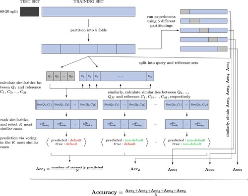
The dataset is apportioned into train and test sets, with an 80–20 split. The fivefold cross-validated grid search is used to optimize the models. Based on the introduction above, the process of evaluating the classification models can be described as follows:

1. Remove the input data with missing values and normalize the data to the range [0,1].

2. Apply the random under-sampling method to generate ten balanced samples for each financial dataset.

3. Train and test multiple classification models and get the measure performances for each generated sample.

4. Calculate the performance scores with paired t -tests.

5. Conduct TOPSIS method to evaluate the relative performance of the classification models.

4. Results

4.1. Empirical evidence

The classification results of eight classifiers on the five financial datasets, evaluated by seven measure metrics, are reported in table 2. The results are calculated in terms of the average measure performance of 10 randomly balanced samples of each dataset. The best result of a specific measure in a specific dataset is highlighted in boldface, and the performance is column-wise colored (the redder, the better). From table 2, no classifier performs the best across all measures for a single dataset or has the best performance for a single measure across all datasets. The results are aligned with the observations from the study of Novaković (2011). However, we can observe that CBR method clearly shows competitive performance among the measures and performs stable across the different data sets. As there is no obvious large gradient variation in most colored columns of datasets, the detection of the statistically significant differences between the performance of two classifiers by the t-test is important.

Table 2. Classification results.

Notes: Color indicates the performance columnwise (the redder, the better). For all statistical measures retained the higher the value, the more is the corresponding model. The best values of each column are depicted in bold.

The performance scores of all classification models are calculated, based on the measure results in table 2, are shown in table 3. For each performance measure, the best score is highlighted in boldface. The higher performance score indicates the classifier performs statistically significantly better than the others for a specific measure over five financial datasets. However, no classifier has the best performance for all measures. The results are consistent with the ones also reported in the research of Peng et al. (2011). Therefore, the MCDM method is required to provide an overall ranking of classification algorithms.

Table 3. Performance scores of algorithms.

	Measure
Algorithm	Accuracy	Precision	Recall	Specificity	F1-score	ROC_AUC	G-mean
LR	7	−3	12	−10	6	7	8
KNN	−18	−8	−19	3	−21	−18	−19
DT	7	8	−5	11	0	6	4
GNB	−13	−4	−3	−5	2	−13	−11
MLP	13	10	1	7	6	13	10
LASSO	−3	−1	2	−3	−3	−2	−1
CBR_EW	−9	−8	−5	−5	−8	−9	−9
CBR_E	16	6	17	2	18	16	18

Notes: With bold, the best value is depicted in each column. The higher performance score indicates the classifier performs statistically significantly better than the others for a specific measure over five financial datasets.

The ranking of the classification models generated by TOPSIS is shown in table 4. From the table, we can see the proposed CBR has the relative best performance. Compared with the naive benchmark equally-weighted CBR model, the performance of the proposed CBR model has been improved considerably. In summary, we can conclude that the proposed data-driven evolutionary CBR has an overall better performance than the other AI classification algorithms for financial risk prediction problems.

Table 4. TOPSIS values.

Algorithm	TOPSIS	Ranking
CBR_E	0.8379	1
MLP	0.7561	2
DT	0.6475	3
LR	0.5685	4
LASSO	0.4593	5
GNB	0.3342	6
CBR_EW	0.2805	7
KNN	0.2024	8

Notes: The table presents the TOPSIS values of all models under study and their related ranking. Higher TOPSIS value is associated with better model performance.

4.2. Interpretation of results

Compared with the other classification methods, one of the important characteristics of CBR is the interpretability of the prediction result. In this section, we conduct a case study with the dataset of the south German credit to show the explainability of the CBR system. The south German credit dataset is publicly available and widely used in the scientific field for research on credit risk prediction, such as the recent studies of Ha et al. (2019), Alam et al. (2020), and Trivedi (2020). The dataset provider offered a detailed description of the features, which are essential information to explain the results. In contrast, the other public datasets used in this paper contain either names of features that are confidential, or a description of features is missing, which makes them not suitable for explainability study. Thus we use the German credit dataset to perform the case study. In this dataset, each entry represents a person who takes credit from a bank. Each person is classified as subject to credit risk or not according to the set of features. The detailed description of features can be found in appendix 8.

4.2.1. Results explanation based on similar cases

Applying the CBR system, a bank can provide reasons/suggestions for consumers who failed in applying for credit from the bank. As aforementioned, case-based explanation will promote confidence in the decision.

For instance, an application case $C_0$ has been correctly classified as a bad credit risk by applying the CBR system (voting from the three most similar cases, the optimal K = 3). Through similarity queries to the cases' base, the three most similar cases of the case $C_0$, $C_1^d$ (default), $C_2^d$ (default), and $C_3^n$ (non-default), and its second most similar good credit risk cases $C_4^n$ (non-default) can be found and their attributes are shown in table 5. From table 5, we can observe that the difference between $C_0$ and its most similar case $C_1^d$ is that the latter has less credit amount and duration. The repayment default of the case $C_1^d$ has a strong indication that case $C_0$ will default. Similarly, the second similar case $C_2^d$ with better attributes (less credit amount, duration, and longer time living in the present residence, and more credits at the current bank) still defaults. Thus, to avoid the potential risk, the bank has a reason to reject similar cases. Meanwhile, two quality cases $C_3^n$ and $C_4^n$ can provide suggestions for the customer to improve his case and obtain a successful application. For the same duration, the less credit amount is important, and even there is a need to lessen the credit installments as a percentage of disposable income to a low level. Besides, considering the age, an important feature aforementioned, longer employment duration, and proof of property are important to decrease the expectation of the credit risk.

Table 5. Features comparison for the south German credit risk.

Feature	$C_0$	$C_1^d$	$C_2^d$	$C_3^n$	$C_4^n$
Status	1	1	1	1	1
Duration	11	9	5	11	11
Credit history	4	4	4	4	4
Purpose	0	0	0	0	0
Amount	3905	2799	3676	3499	691
Savings	1	1	1	1	1
Employment duration	3	3	3	3	5
Installment rate	2	2	1	3	4
Personal status	3	3	3	2	3
Other debtors	1	1	1	2	1
Present residence	2	2	3	2	3
Property	1	1	1	1	2
Age	36	36	37	28	35
Other installment plans	3	3	3	3	3
Housing	1	1	1	2	2
Number credits	2	2	3	2	2
Job	3	3	3	3	3
People liable	1	1	1	2	2
Telephone	1	1	1	1	1
Foreign worker	2	2	2	2	2

Notes: What the value of the features stands for can be found in appendix 8. $C_0$ is the application case which has been predicted as that there is a possibility of a loss resulting from the applier's failure to meet contractual obligations. $C_1^d$ (1st), $C_2^d$ (2nd), and $C_3^n$ (3rd) are three most similar cases with $C_0$. $C_1^d$ and $C_2^d$ are two default cases. $C_3^n$ and $C_4^n$ are the most two similar quality cases. Superscript d and n stand for default and non-default cases, respectively.

4.2.2. Results explanation based on probability

The application case $C_0$ is classified in terms of voting its three most similar cases. According to the log likelihood function introduced in section 2.2.2, we can obtain the probability weights of the most, second, third similar cases $C_1^d$, $C_2^d$, and $C_3^n$ are 0.4879, 0.3123, and 0.1998, respectively. Thus there is 80.02% probability that $C_0$ is a bad case. The bank has a high confidence to reject the application.

4.2.3. Results explanation based on feature relevance

The global similarity is calculated in terms of the relevance scores of features. Table 6 shows the different feature relevance when making a prediction for the risk of credit applications. From table 6, we can observe that the financial status is the most important feature. The second is the duration that the customer wants to take the credit from a bank. The third and fourth ones are credit amount and age, respectively. In contrast, whether the applier is a foreign worker are not relatively important. Understanding the relevance of the features is significant for a bank to filter applications and make approval decisions.

Table 6. Feature relevance for the south German credit risk.

Feature	Feature relevance (%)	Feature	Feature relevance (%)
Status	13.84	Present residence	4.91
Duration	7.01	Property	4.72
Credit history	5.65	Age	6.07
Purpose	5.57	Other installment plans	3.61
Amount	6.60	Housing	3.88
Savings	4.82	Number credits	3.57
Employment duration	5.48	Job	4.34
Installment rate	4.93	People liable	2.82
Personal status	4.21	Telephone	3.33
Other debtors	3.25	Foreign worker	1.38

Notes: The tables presents the relevance of each feature. The sum of all the value is equal to 100.

As aforementioned, we use a CID tree to detect the most likely causes for a default case. The decision tree is built using the C4.5 algorithm, and the prominent features have been highlighted (node P (blue) and node S (yellow)), as shown in figure 1, and the score for each node is calculated based on equation (9(9) $\mathrm{S}\mathrm{c}\mathrm{o}\mathrm{r}{\mathrm{e}}_{\mathrm{p}}=({\mathrm{D}}_{\mathrm{p}}^2{\mathrm{N}}_{\mathrm{s}}^2\left)/\right({\mathrm{N}}_{\mathrm{p}}^2{\mathrm{D}}_{\mathrm{s}}^2)$(9) ), as shown in table 7. From figure 1 and table 7, we can observe that the inferior status of checking account, bad credit history, and too many people liable of credit applicants are the three most likely causes for their cases default. Compared with numeric features, such as the duration and amount, the three categorical and ordinal features perform better for discriminating default and non-default cases. Thus a creditor is able to determine if an applicant is a good credit risk based on the following criterion:

• The status of the credit applicants' checking account with the bank is essential to be active with a positive balance.

• Credit applicants with defective credit history have a high possibility of default again.

• The fewer the number of persons who financially depend on a credit applicant, the better.

Figure 1. The most likely causes for a particular default based on CID tree scoring. The decision tree is built using the C4.5 algorithm, and the prominent features have been highlighted (node P (blue) and node S (yellow)).

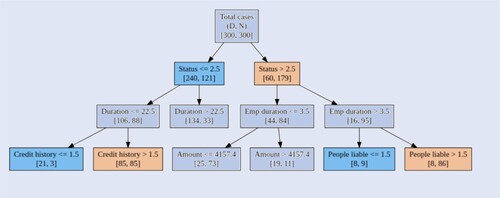
Table 7. The scores obtained from CID.

Feature	D	N	Score	1/Score
Total cases	300	300	0	0
Status < 2.5	240	121	35.0	0.0
Status > 2.5	69	179	0.0	35.0
Duration < 2.5	106	88	0.1	11
Duration >22.5	134	33	11	0.1
Employment duration < 3.5	44	84	9.7	0.1
Employment duration >3.5	16	95	0.1	9.7
Credit history < 1.5	21	3	81	0.0
Credit history >1.5	85	85	0.0	81
Amount < 4157.4	25	73	0.0	25.4
Amount $>4157.4$	19	11	25.4	0.0
People liable < 1.5	86	8	95.6	0.0
People liable $>1.5$	8	86	0.0	95.6

The CID tree provides complementary information for CBR system to detect the causes of default cases.

4.2.4. Further information detection

According to the feature relevance analysis above, we know features have different contributions when determining if a credit applicant is qualified. Typically, status, credit history, and people liable are the three most likely decisive reasons, for all of which a higher value is better. In this section, we implement the clustering technique to extract more criteria for credit application decision-making by using group information from the three salient features.

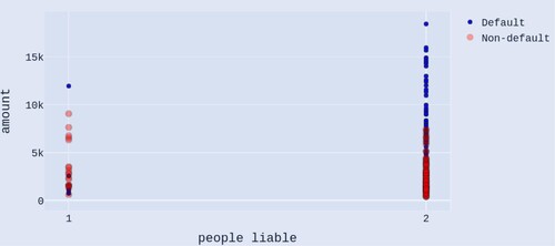
Due to the features with varying degrees of magnitude and range, we normalized their value on a scale of 0–1. Consequently, the overall score of each case (sum value of the three features) ranges from 0 to 3. The relations between the overall score and the rate of good cases can be found in figure 2. In addition, the customer segmentation is useful in understanding demographic and psychographic profiles of the credit applicants in a bank (Zakrzewska and Murlewski 2005). We cluster the cases into three groups using k-means algorithm and highlight each group with different colors, shown in figure 2. From the figure, we can see that the non-default rate of the low value group is steadily less than 53% while the moderate and high value group increases significantly. Compared to the low value group (high probability to default) and high value group (low probability to default), the moderate group has the high potential to increase the rate of good cases with cost-effective assists from the bank. The applicants in moderate group deserve the priority from bank to conduct group analysis and offer constructive advice to escalate the likelihood of their successful applications. To further detect information for credit application decision making, the scatterplots, duration and status, duration and credit history and amount and people liable of the cases data from the moderate group, are shown in figures 3, 4 and 5, respectively. Blue color dots denote default cases and red dots denote non-default.

Figure 2. The rate of good cases increases with the overall score of cases increases. Green, blue, and red areas stand for the low, moderate, and high value groups, respectively.

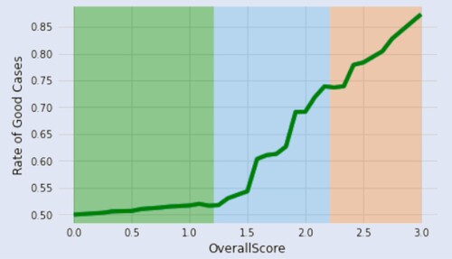
Figure 3. Scatterplot of duration and status of the cases data from the moderate group, with blue and red colors denoting default and non-default, respectively.

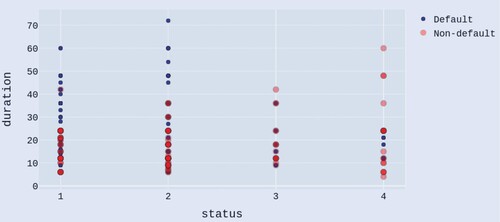
Figure 4. Scatterplot of duration and credit history of the cases data from the moderate group, with blue and red colors denoting default and non-default, respectively.

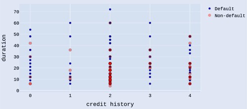
Figure 5. Scatterplot of amount and people liable of the cases data from the moderate group, with blue and red colors denoting default and non-default, respectively.

From figure 3, we can see that if the value of duration excesses some value, the majority of application cases are default when the status of checking accounts of customers is not active with a positive balance (status = 1 or 2). This can direct the bank by setting thresholds to effectively filter and review cases in a preliminary stage. In addition, the reduction of credit application duration would be a constructive suggestion in a quantitative way for a particular customer to improve his application when his financial status is not competent.

From figure 4, we can observe that it is meaningful to set a decisive threshold to reject credit application with a long duration requirement when the debtor has no history of credits taken or all credits paid back duly (credit history = 2). Meanwhile, if the debtor has a delayed history of paying off or a critical account elsewhere, he has a high probability of defaulting with any duration magnitude. There are no obvious relations between the duration and creditability of a debtor when he has all credits at this bank paid back duly. It is interesting to note that if the credit applicant has existing credits paid back duly till now, the short duration is not a good signal. The present applied credit would be abused for repayment.

In figure 5, we can see that the majority of the credit applicants in the moderate group have less than 2 people who financially depend on them. And, it is obvious that there is a decision threshold for approving credit, considered in terms of amount, when 0–2 people are financially supported by the applicant.

5. Conclusion

Financial risks are uncertainties associated with financial decisions, such as credit application approval and bank customers' churn reduction. In recent years, some complex black-box AI methods have achieved unprecedented levels of performance when learning to solve increasing complex computational tasks, including financial risk detection. However, the GDPR rule in Europe contests any automated decision-making that was made on a solely algorithmic basis. Additionally, decision-making processes are required to be accompanied by a meaningful explanation. Consequently, financial industries guided by the regulation urge the need for innovative research on XAI methods. CBR system is an XAI method, which has been identified as a useful method in real-life applications.

In this study, a data-driven explainable CBR system is proposed for solving financial risk prediction problems. In particular, feature relevance scoring methods are applied for assigning global similarity weights for attributes, and the PSO algorithm is employed for optimizing the parameters of local similarity functions. The proposed data-driven approach provides a way to overcome the drawback of the standard CBR system, which highly depends on domain knowledge and prior experience when building a successful model. The experimental results show that the proposed CBR method has a relatively superior prediction performance compared to the widely used classification machine learning methods. In addition, compared to other black-box machine learning methods, the CBR system is capable of interpreting the result of the financial risk prediction, and further detects the schemes to decrease or avoid financial risk. This characteristic is significantly helpful for both financial institutions and their customers. In particular, we introduce four major explanation goals and conduct an experiment to outline a unified view on explanation in the CBR system, using a German credit risk dataset. The results show the scheme to explain the decision making process based on the CBR system and explore more decisive information for the bank.

Several extensions of the current study can be developed. In the proposed CBR system, the design of global similarity depends on the existing feature scoring methods. In further research, we will explore a general way to detect the optimal feature weights. Furthermore, the main limitation of the proposed CBR system is that its training is extremely time-consuming. The PSO algorithm is a computationally-intensive optimization method to search for the parameters of local similarity functions. More efficient optimization algorithms for creating the CBR system are needed. In addition, homogeneous and heterogeneous CBR ensemble systems to enhance forecasting accuracy can be investigated. Moreover, the balance between complexity and explainability of predictive models is subject to further research. Finally, the study was carried out using the five financial risk datasets, but the generality of the proposed CBR system ensures a possible application to other decision-support systems.

Acknowledgments

This work acknowledges research support by COST Action ‘Fintech and Artificial Intelligence in Finance—Towards a transparent financial industry’ (FinAI) CA19130. Critical comments and advice from Denis M. Becker, Christian Ewald, Wolfgang Karl Härdle, Steven Ongena, and Endre Jo Reite are gratefully acknowledged. The computations were performed on resources provided by UNINETT Sigma2—the National Infrastructure for High Performance Computing and Data Storage in Norway.

Disclosure statement

No potential conflict of interest was reported by the author(s).

Appendices

Appendix 1.

Simple example of CBR

Assume there are two persons (Q and C) who have three (L = 3) equally-weighted features ($w_j=1/3$): weight, height, and age as shown in table A1. In addition, among all the people (dataset), the highest and lowest values of weight, height, and age are known as well. The parameters $a_1$, $a_2$, $a_3$, $b_1$, $b_2$, and $b_3$ in equation (1(1) $\mathrm{S}\mathrm{i}\mathrm{m}(Q,C)=\sqrt{\sum _{j=1}^L{w}_j{\left[{\mathrm{s}\mathrm{i}\mathrm{m}}_j\right(q_j,c_j\left)\right]}^2}$(1) ) are assumed to be 3, 2, 1, 1, 2, and 3, respectively. The similarity calculation of Q and C based on those features based on equations (1(1) $\mathrm{S}\mathrm{i}\mathrm{m}(Q,C)=\sqrt{\sum _{j=1}^L{w}_j{\left[{\mathrm{s}\mathrm{i}\mathrm{m}}_j\right(q_j,c_j\left)\right]}^2}$(1) ) and (2(2) ${\mathrm{s}\mathrm{i}\mathrm{m}}_j(q_j,c_j)=\{\begin{array}{ll}{\left[{\displaystyle \frac{D_j-(c_j-q_j)}{D_j}}\right]}^{{\mathit{a}}_{\mathit{j}}},& \mathrm{i}\mathrm{f}{q}_j\le c_j\\ {\left[{\displaystyle \frac{D_j-(q_j-c_j)}{D_j}}\right]}^{{\mathit{b}}_{\mathit{j}}},& \mathrm{i}\mathrm{f}{q}_j>c_j\end{array}$(2) ) is given by $\begin{array}{rl}{\mathrm{s}\mathrm{i}\mathrm{m}}_1(q_1,c_1)& ={\left[\frac{D_1-(q_1-c_1)}{D_1}\right]}^{{\mathit{b}}_{\mathbf{1}}}\\ & ={\left[\frac{100-(120-100)}{100}\right]}^{\mathbf{1}}=0.8\\ {\mathrm{s}\mathrm{i}\mathrm{m}}_2(q_2,c_2)& ={\left[\frac{D_2-(q_2-c_2)}{D_2}\right]}^{{\mathit{b}}_{\mathbf{2}}}\\ & ={\left[\frac{50-(180-170)}{50}\right]}^{\mathbf{2}}=0.64\\ {\mathrm{s}\mathrm{i}\mathrm{m}}_3(q_3,c_3)& ={\left[\frac{D_3-(c_3-q_3)}{D_3}\right]}^{{\mathit{a}}_{\mathbf{3}}}\\ & ={\left[\frac{40-(40-35)}{40}\right]}^{\mathbf{1}}=0.875\\ \mathrm{S}\mathrm{i}\mathrm{m}(Q,C)& =\sqrt{\sum _{j=1}^3{w}_j{\left[{\mathrm{s}\mathrm{i}\mathrm{m}}_j\right(q_j,c_j\left)\right]}^2}\\ & =\sqrt{\frac{\mathbf{1}}{\mathbf{3}}{\left[0.8\right]}^2+\frac{\mathbf{1}}{\mathbf{3}}{\left[0.64\right]}^2+\frac{\mathbf{1}}{\mathbf{3}}{\left[0.875\right]}^2}=0.7779\end{array}$

Table A1. The features of Person Q and C.

	Weight	Height	Age
Person Q	120 ($q_1$)	180 ($q_2$)	35 ($q_3$)
Person C	100 ($c_1$)	170 ($c_2$)	40 ($c_3$)
Maximum	180	200	60
Minimum	80	150	20
Difference between Max and Min ($D_j$)	100 ($D_1$)	50 ($D_2$)	40 ($D_3$)

Appendix 2.

PSO

PSO is a computational method that optimizes a problem by iteratively improving a solution measured in a certain metric. The basic idea is that a population of particles moves through the search space. Each particle has knowledge about its current velocity, its own past best configuration ($\overrightarrow{p}\left(t\right)$), and the current global best solution ($\overrightarrow{g}\left(t\right)$). Based on this information, each particle's velocity is updated such that it moves closer to the global best and its past best solution at the same time. The velocity update is performed according to the following equation: (A1) $\overrightarrow{v}(t+1)=\omega \overrightarrow{v}\left(t\right)+c_1{r}_1\left(\overrightarrow{p}\right(t)-\overrightarrow{x}(t\left)\right)+c_2{r}_2\left(\overrightarrow{g}\right(t)-\overrightarrow{x}(t\left)\right)$(A1) where $c_1$ and $c_2$ are constants defined beforehand that determine the significance of $\overrightarrow{p}\left(t\right)$ and $\overrightarrow{g}\left(t\right)$. $\overrightarrow{v}\left(t\right)$ is the velocity of the particle, $\overrightarrow{x}\left(t\right)$ is the current particle position, $r_1$ and $r_2$ are random numbers from the interval [0,1], and ω is a constant ($0\le \omega \le 1$). The new position is calculated by summing the previous position and the new velocity as follows: (A2) $\overrightarrow{x}(t+1)=\overrightarrow{x}\left(t\right)+\overrightarrow{v}(t+1)$(A2) In each iteration, if the best individual solution is better than the global best solution, which will be updated by the best individual solution. This iterative process is repeated until a stopping criterion is satisfied. In the proposed CBR system, PSO is used to search for the optimal parameters for each feature similarity function. The applied configuration of PSO is [$c_1$: 1.5, $c_2$: 1.5, w: 0.8] and the stop condition is satisfied after 1000 iterations. The population size of particles is varied and initialized as the size of features.

Appendix 3.

Parallel computing

Parallel computing is a type of computation where large calculations can be divided into smaller ones, and their computing processes are carried out simultaneously. The potential speedup of an algorithm on a parallel computing framework is given by Amdahl's law, which can be expressed mathematically as follows: (A3) $\mathrm{S}\mathrm{p}\mathrm{e}\mathrm{e}\mathrm{d}\mathrm{u}\mathrm{p}=\frac{1}{(1-p)+\frac{p}{s}}$(A3) where Speedup is the theoretical maximum speedup of the execution of the whole task, p is the proportion of a system or program that can be made parallel, and s stands for the number of processors.

One successful application of GPU-based parallel computing is deep learning, which is a typical intensive computing and training task that can be split. For the CBR querying process, it also can be paralleled. In particular, the similarity calculation between a query and each case can be processed simultaneously. The algorithm for predicting N queries with L features (query matrix) based on M cases with L features (reference matrix) is shown as follows:

The computation time for querying the test set of the five financial datasets is shown in table A2. The graphics processing unit (GPU) used in this study is the NVIDIA Geforce GTX 1080. From table A2, we can observe that the query time increases with increasing magnitude of data.

Table A2. Query time instances of the datasets used in cross-validation.

	CCF	CCD	GCA	BC	FD
Query time (s)	0.0147	2.3931	0.0053	0.1586	0.0036
Total cases	984	13,272	600	4,074	272
Reference cases	787	10,617	480	3,259	217
Query cases	197	2,655	120	815	55
Features number	30	24	20	10	83

Notes: The randomly under-sampling cases data is apportioned into reference and query, with an 80–20 split. The fivefold cross-validation is used to evaluate the CBR system performance when training model.

Appendix 4.

Cost function

The cost function is non-differentiable. Thus PSO is applied for the optimization since the algorithm does not require the optimization problem to be differentiable as is required by classic optimization methods, such as gradient descent used in training neural networks. The illustration of the cost function can be seen in figure A1.

Appendix 5.

Benchmark models

The benchmark models are briefly introduced as follows:

A.1. Logistic regression

Logistic regression is a mathematical modeling approach that can be used to describe the relationship of several variables to a dichotomous dependent variable (Kleinbaum 1994). It is an efficient and powerful way to analyze the effect of a group of independent variables on a binary outcome (Stoltzfus 2011). In logistic regression, regularization is used to reduce generalization error and preventing the algorithm from overfitting in feature rich dataset. The Ridge and LASSO methods are most commonly used. Consequently, the inverse of regularization strength is also needed to determine. The smaller values specify stronger regularization. The best model can be found by cross-validation grid search.

A.2. k-nearest neighbor

k-nearest neighbors algorithm is a non-parametric classification method, which means it does not make any assumption on underlying data. It only considers the k-nearest neighbors to classify the query point (Mitchell 1997). The hyperparameter required to decide is the k. The best model is achieved through a cross-validation procedure by using a grid search for the k. The applied value of the k ranges from 1 to 20.

A.3. Decision tree

A decision tree is a map of the possible outcomes of a series of related choices, where each internal choice (node) denotes a test on an attribute, each branch represents an outcome of the test, and each leaf node holds a class label (Song and Lu 2015). There are several hyperparameters required to tune. Impurity is used to determine how decision tree nodes are split. Information gain and Gini Impurity are commonly used. The maximum depth of the tree and the minimum number of samples required to be at a leaf node are also important to tune. They are used to prevent a tree from overfitting. The pre-pruning method is typically used and the growth of trees stops by setting the constraints. The applied values of the maximum depth and minimum samples range from 2 to 10 and 5 to 10, respectively. Cross-validation grid search is applied to find the optimal model.

Figure A1. Illustration of the cost function.

The cost function is the average prediction accuracy calculated based a fivefold cross-validation, used for the prediction performance evaluation of a CBR system $\mathrm{S}\mathrm{i}\mathrm{m}(Q,C)$ with specific parameters (K, $w_j$, $a_j$, $b_j$). The training set is partitioned into five folds (one for query and four for reference sets) to run five experiments. For each experiment, each $Q_n$ (n = 1,…, N) from the query set will be used to calculate its similarities with all $C_m$ (m = 1,…, M) from the reference set. For instance, for $Q_1$, the similarities $\mathrm{S}\mathrm{i}\mathrm{m}(Q_1,C_1)$, $\mathrm{S}\mathrm{i}\mathrm{m}(Q_1,C_2)$,…, $\mathrm{S}\mathrm{i}\mathrm{m}(Q_1,C_M)$ will be calculated. Then those similarities will be ranked, and the K cases $C_{{\mathrm{R}\mathrm{a}\mathrm{n}\mathrm{k}}_1}^{Q_1}$, $C_{{\mathrm{R}\mathrm{a}\mathrm{n}\mathrm{k}}_2}^{Q_1}$,…, $C_{\mathrm{R}\mathrm{a}\mathrm{n}{\mathrm{k}}_{\mathrm{K}}}^{Q_1}$ with highest similarities values will be selected. The prediction for $Q_1$ will be made based on the voting in the labels of those K cases. Similarly, the predictions for $Q_2$, $Q_3$,…, and $Q_N$ can be obtained. Afterwards, the accuracy of the prediction in this experiment $\mathbf{A}\mathbf{c}{\mathbf{c}}_{\mathbf{1}}$ can be calculated, which is equal to $\mathbf{n}\mathbf{u}\mathbf{m}\mathbf{b}\mathbf{e}\mathbf{r}\mathbf{o}\mathbf{f}\mathbf{c}\mathbf{o}\mathbf{r}\mathbf{r}\mathbf{e}\mathbf{c}\mathbf{t}\mathbf{l}\mathbf{y}\mathbf{p}\mathbf{r}\mathbf{e}\mathbf{d}\mathbf{i}\mathbf{c}\mathbf{t}\mathbf{e}\mathbf{d}/\mathbf{N}$. Similarly, $\mathbf{A}\mathbf{c}{\mathbf{c}}_{\mathbf{2}}$, $\mathbf{A}\mathbf{c}{\mathbf{c}}_{\mathbf{3}}$, $\mathbf{A}\mathbf{c}{\mathbf{c}}_{\mathbf{4}}$, and $\mathbf{A}\mathbf{c}{\mathbf{c}}_{\mathbf{5}}$ for the other experiments can be computed. Last, the prediction performance for the CBR with the specific parameters can be evaluated by $\mathbf{A}\mathbf{c}\mathbf{c}\mathbf{u}\mathbf{r}\mathbf{a}\mathbf{c}\mathbf{y}$, which is equal to $\mathbf{(}\mathbf{A}\mathbf{c}{\mathbf{c}}_{\mathbf{1}}\mathbf{+}\mathbf{A}\mathbf{c}{\mathbf{c}}_{\mathbf{2}}\mathbf{+}\mathbf{A}\mathbf{c}{\mathbf{c}}_{\mathbf{3}}\mathbf{+}\mathbf{A}\mathbf{c}{\mathbf{c}}_{\mathbf{4}}\mathbf{+}\mathbf{A}\mathbf{c}{\mathbf{c}}_{\mathbf{5}}\mathbf{)}\mathbf{/}\mathbf{5}$.

A.4. Gaussian naive Bayes

Naive Bayes Classifiers are based on the Bayesian rule and probability theorems and has a strong assumption that predictors should be independent of each other (Mitchell 1997). Gaussian naive Bayes classification is an extension of naive Bayes method with an assumption that the continuous values associated with each class are distributed according to a Gaussian distribution. No hyperparameter tuning is required in Gaussian naive Bayes.

A.5. Multilayer perceptron

A Multilayer preceptron (MLP) is a class of feedforward artificial neural network (ANN), which consists of at least three layers of nodes: an input layer, a hidden layer, and an output layer (Gardner and Dorling 1998). It is a supervised non-linear learning algorithm for either classification or regression. MLP requires tuning a number of hyperparameters such as the number of hidden neurons, layers, and iterations. The applied hidden layers range from 2 to 10. For each layer, the units range from 32 to 512. The training dataset is apportioned into train and validation sets, with an 80–20 split. The hyperband algorithm is used for hyperparameters optimization (Li et al. 2018). The ANN with the optimal topology is applied for each dataset to test the performance.

A.6. LASSO regression

LASSO regression is a linear regression method that performs both feature selection and regularization to enhance the prediction accuracy. The goal of the algorithm is to minimize: $\sum _{j=1}^m(y_j-\sum _{i=1}^n{x}_{ji}{\text{β}}_i{)}^2+\lambda \sum _{i=1}^n|w_i|$, where w is the vector of model coefficients and λ is a hyperparameter (Tibshirani 1996). The algorithm has the advantage that it shrinks some of the less critical coefficients of features to zero and λ is basically the amount of shrinkage. The best model is selected by cross-validation.

Appendix 6.

Measure metrics

TP (true positive) is the number of correctly classified positive instances. TN (true negative) is the number of correctly classified negative instances. FP (false positive) is the number of positive instances misclassified. FN (false negative) is the number of negative instances misclassified.

1. Precision is referred to as the positive predictive value. The equation is represented as follows: (A4) $\mathrm{P}\mathrm{r}\mathrm{e}\mathrm{c}\mathrm{i}\mathrm{s}\mathrm{i}\mathrm{o}\mathrm{n}=\frac{\mathrm{T}\mathrm{P}}{\mathrm{T}\mathrm{P}+\mathrm{F}\mathrm{P}}$(A4)

2. Recall or sensitivity is referred to as the true positive rate. The equation is represented as follows: (A5) $\mathrm{R}\mathrm{e}\mathrm{c}\mathrm{a}\mathrm{l}\mathrm{l}=\frac{\mathrm{T}\mathrm{P}}{\mathrm{T}\mathrm{P}+\mathrm{F}\mathrm{N}}$(A5)

3. Specificity is referred to as the true negative rate. The equation is represented as follows: (A6) $\mathrm{S}\mathrm{p}\mathrm{e}\mathrm{c}\mathrm{i}\mathrm{f}\mathrm{i}\mathrm{c}\mathrm{i}\mathrm{t}\mathrm{y}=\frac{\mathrm{T}\mathrm{N}}{\mathrm{F}\mathrm{P}+\mathrm{T}\mathrm{N}}$(A6)

4. F1-score or F-measure is the harmonic mean of precision and recall. The equation is represented as follows: (A7) $\mathrm{F}1\text{-}\mathrm{s}\mathrm{c}\mathrm{o}\mathrm{r}\mathrm{e}=2\times \frac{\mathrm{p}\mathrm{r}\mathrm{e}\mathrm{c}\mathrm{i}\mathrm{s}\mathrm{i}\mathrm{o}\mathrm{n}\times \mathrm{r}\mathrm{e}\mathrm{c}\mathrm{a}\mathrm{l}\mathrm{l}}{\mathrm{p}\mathrm{r}\mathrm{e}\mathrm{c}\mathrm{i}\mathrm{s}\mathrm{i}\mathrm{o}\mathrm{n}+\mathrm{r}\mathrm{e}\mathrm{c}\mathrm{a}\mathrm{l}\mathrm{l}}$(A7)

5. ROC_AUC (the area under the receiver operating characteristic) shows how much a model is capable of distinguishing between classes. Higher the AUC, better the model is.

6. G-mean is the geometric mean of recall and precision. The equation is represented as follows: (A8) $\mathrm{G}\text{-}\mathrm{m}\mathrm{e}\mathrm{a}\mathrm{n}=\sqrt{\mathrm{r}\mathrm{e}\mathrm{c}\mathrm{a}\mathrm{l}\mathrm{l}\times \mathrm{p}\mathrm{r}\mathrm{e}\mathrm{c}\mathrm{i}\mathrm{s}\mathrm{i}\mathrm{o}\mathrm{n}}$(A8)

Appendix 7.

Technique for order preference by similarity to ideal solution (TOPSIS)

The procedure of TOPSIS can be summarized as follows:

1. Calculate the normalized decision matrix. The normalized value $r_{ij}$ is calculated as (A9) $r_{ij}=x_{ij}/\sqrt{\sum _{i=1}^n{x}_{ij}^2},i=1,\dots ,n;j=1,\dots ,m,$(A9) where n and m denote the number of alternative models and the number of criteria, respectively. For alternative model $A_i$, the performance score of the jth criterion $C_j$ is represented by $x_{ij}$.

2. The weighted normalized decision matrix is calculated as follows: (A10) $v_{ij}=w_j{r}_{ij},i=1,\dots ,n;j=1,\dots ,m,$(A10) where $w_j$ is the weight of the jth criterion obtained by the information entropy approach. To minimize the input of decision maker, we consider the criterion are equally important.

3. The ideal alternative solution $A^{+}$ is calculated as (A11) $A^{+}=\{v_1^{+},\dots ,v_m^{+}\}=\left\{\right(\underset{i}{max}{v}_{ij}|j)\in I^{\mathrm{\prime }}),\left(\underset{i}{min}{v}_{ij}|j\right)\in I^{\mathrm{\prime }\mathrm{\prime }}\}$(A11) where $I^{\mathrm{\prime }}$ denotes benefit criteria and $I^{\mathrm{\prime }\mathrm{\prime }}$ denotes cost criteria.

4. The anti-ideal alternative solution $A^{-}$ is calculated as (A12) $A^{-}=\{v_1^{-},\dots ,v_m^{-}\}=\left\{\right(\underset{i}{min}{v}_{ij}|j)\in I^{\mathrm{\prime }}),\left(\underset{i}{max}{v}_{ij}|j\right)\in I^{\mathrm{\prime }\mathrm{\prime }}\}$(A12)

5. The distance of each alternative from the ideal alternative solution $A^{+}$ is calculated as (A13) $D_i^{+}=\sqrt{\sum _{j=1}^m(v_{ij}-v_j^{+}{)}^2},i=1,\dots ,n$(A13) The distance of each alternative from the anti-ideal alternative solution $A^{-}$ is calculated as (A14) $D_i^{-}=\sqrt{\sum _{j=1}^m(v_{ij}-v_j^{-}{)}^2},i=1,\dots ,n$(A14)

6. The relative model degree is calculated as (A15) $R^{+}=D_i^{-}/(D_i^{-}+D_i^{+}),i=1,\dots ,n$(A15) where the degree $R^{+}$ presents the relative rank of alternative models (the larger, the better).

Appendix 8.

The description of the south German credit data

The detailed explanation of the features of the south German credit dataset is presented in table A3.

Table A3. The description of the south German credit data (Grömping 2019).

Feature	Description	Level
Status	Status of the debtor's checking account with the bank	1: no checking account, 2: ‘$\cdots <0$ DM’, 3: ‘$0<=\cdots <200$ DM’, 4: ‘$\cdots >=200$ DM / salary for at least 1 year’
Duration	Credit duration in months	Numeric
Credit history	History of compliance with previous or concurrent credit contracts	0: ‘delay in paying off in the past’, 1: ‘critical account/other credits elsewhere’, 2: ‘no credits taken/all credits paid back duly’, 3: ‘existing credits paid back duly till now’, 4: ‘all credits at this bank paid back duly’
Purpose	Purpose for which the credit is needed	0: ‘others’, 1: ‘car (new)’, 2: ‘car (used)’, 3: ‘furniture/equipment’, 4: ‘radio/television’, 5: ‘domestic appliances’, 6: ‘repairs’, 7: ‘education’, 8: ‘vacation’, 9: ‘retraining’, 10: ‘business’
Amount	Credit amount in DM	Numeric
Savings	Debtor's savings	1: ‘unknown/no savings account’, 2: ‘$\cdots <100$ DM’, 3: ‘$100<=\cdots <500$ DM’, 4: ‘$500<=\cdots <1000$ DM’, 5: ‘$\cdots >=1000$ DM’
Employment duration	Duration of debtor's employment with current employer	1: ‘unemployed’, 2: ‘< 1 yr’, 3: ‘$1<=\cdots <4$ yrs’, 4: ‘$4<=\cdots <7$ yrs’, 5: ‘$>=7$ yrs’
Installment rate	Credit installments as a percentage of debtor's disposable income	1: ‘$>=35$’, 2: ‘$25<=\cdots <35$’, 3: ‘$20<=\cdots <25$’, 4: ‘$<20$’
Personal status	Combined information on sex and marital status	1: ‘male : divorced/separated’, 2: ‘female 1: non-single or male : single’, 3: ‘male : married/widowed’, 4: ‘female : single’
Other debtors	Is there another debtor or a guarantor for the credit?	1: ‘none’, 2: ‘co-applicant’, 3: ‘guarantor’
Present residence	Length of time (in years) the debtor lives in the present residence	1: ‘$<1$ yr’, 2: ‘$1<=\cdots <4$ yrs’, 3: ‘$4<=\cdots <7$ yrs’, 4: ‘$>=7$ yrs’
Property	The debtor's most valuable property	1; ‘unknown / no property’, 2: ‘car or other’, 3: ‘building soc. savings agr./life insurance’, 4: ‘real estate’
Age	Age in years	Numeric
Other installment plans	installment plans from providers other than the credit-giving bank	1: ‘bank’, 2: ‘stores’, 3: ‘none’
Housing	Type of housing the debtor lives in	1: ‘for free’, 2: ‘rent’, 3: ‘own’
Number credits	Number of credits including the current one the debtor has (or had) at this bank	1: ‘1’, 2; ‘2–3’, 3: ‘4–5’, 4: ‘$>=6$’
Job	Quality of debtor's job	1: ‘unemployed/unskilled – non-resident’, 2: ‘unskilled – resident’, 3: ‘skilled employee/official’, 4: ‘manager/self-empl./highly qualif. employee’
People liable	Number of persons who financially depend on the debtor	1: ‘3 or more’, 2: ‘0 to 2’
Telephone	Is there a telephone landline registered on the debtor's name?	1: ‘no’, 2: ‘yes (under customer name)’
Foreign worker	Is the debtor a foreign worker?	1: ‘yes’, 2: ‘no’

References

- Aamodt, A. and Plaza, E., Case-based reasoning: Foundational issues, methodological variations, and system approaches. AI Commun., 1994, 7, 39–59.
- Aamodt, A., Sandtorv, H.A. and Winnem, O.M., Combining case based reasoning and data mining – a way of revealing and reusing rams experience. In Safety and Reliability; Proceedings of ESREL '98, edited by S. Lydersen, G.K. Hansen, H. Sandtorv, pp. 16–19, 1998 (Balkena: Rotterdam).
- Abdou, H., Pointon, J. and El-Masry, A., Neural nets versus conventional techniques in credit scoring in Egyptian banking. Expert Syst. Appl., 2008, 35, 1275–1292.
- Ahn, H. and Jae Kim, K., Bankruptcy prediction modeling with hybrid case-based reasoning and genetic algorithms approach. Appl. Soft Comput., 2009, 9, 599–607.
- Alam, T.M., Shaukat, K., Hameed, I.A., Luo, S., Sarwar, M.U., Shabbir, S., Li, J. and Khushi, M., An investigation of credit card default prediction in the imbalanced datasets. IEEE. Access., 2020, 8, 201173–201198.
- Arshadi, N. and Jurisica, I., Data mining for case-based reasoning in high-dimensional biological domains. IEEE Trans. Knowl. Data Eng., 2005, 17, 1127–1137.
- Atiya, A.F., Estimating the posterior probabilities using the k-nearest neighbor rule. Neural Comput., 2005, 17, 731–740.
- Bach, K. and Althoff, K.D., Developing case-based reasoning applications using mycbr 3. In Case-based reasoning research and development, edited by B.D. Agudo, I. Watson, pp. 17–31, 2012 (Springer: Berlin, Heidelberg).
- Barredo Arrieta, A., Díaz-Rodríguez, N., Del Ser, J., Bennetot, A., Tabik, S., Barbado, A., Garcia, S., Gil-Lopez, S., Molina, D., Benjamins, R., Chatila, R. and Herrera, F., Explainable artificial intelligence (xai): Concepts, taxonomies, opportunities and challenges toward responsible ai. Inf. Fusion, 2020, 58, 82–115.
- Bensic, M., Sarlija, N. and Zekic-Susac, M., Modelling small-business credit scoring by using logistic regression, neural networks and decision trees. Intell. Syst. Account. Finance Manag., 2005, 13, 133–150.
- Brown, C.E. and Gupta, U.G., Applying case-based reasoning to the accounting domain. Intell. Syst. Account. Finance Manag., 1994, 3, 205–221.
- Brunette, E.S., Flemmer, R.C. and Flemmer, C.L., A review of artificial intelligence. In 2009 4th International Conference on Autonomous Robots and Agents, pp. 385–392, 2009 (IEEE: Wellington).
- Bryant, S.M., A case-based reasoning approach to bankruptcy prediction modeling. Intell. Syst. Account. Finance Manag., 1997, 6, 195–214.
- Byanjankar, A., Heikkilä, M. and Mezei, J., Predicting credit risk in peer-to-peer lending: A neural network approach. In 2015 IEEE Symposium Series on Computational Intelligence, pp. 719–725, 2015 (IEEE: Cape Town).
- Ceriani, L. and Verme, P., The origins of the gini index: Extracts from variabilità e mutabilità (1912) by Corrado Gini. J. Econ. Inequal., 2012, 10, 421–443.
- Chi, R.T., Chen, M. and Kiang, M.Y., Generalized case-based reasoning system for portfolio management. Expert Syst. Appl., 1993, 6, 67–76.
- Cost, S. and Salzberg, S., A weighted nearest neighbor algorithm for learning with symbolic features. Mach. Learn., 1993, 10, 57–78.
- Cunningham, P., Doyle, D. and Loughrey, J., An evaluation of the usefulness of case-based explanation. In Case-Based Reasoning Research and Development, edited by K.D. Ashley, D.G. Bridge, pp. 122–130, 2003 (Springer Berlin Heidelberg: Berlin, Heidelberg).
- Dahiya, S., Handa, S. and Singh, N., A feature selection enabled hybrid-bagging algorithm for credit risk evaluation. Expert Syst., 2017, 34, e12217.
- Dal Pozzolo, A., Caelen, O., Le Borgne, Y.A., Waterschoot, S. and Bontempi, G., Learned lessons in credit card fraud detection from a practitioner perspective. Expert Syst. Appl., 2014, 41, 4915–4928.
- Ebrahimi, Kaggle Financial Distress Prediction, 2017. Available at: https://www.kaggle.com/shebrahimi/financial-distress.
- Fayyad, U., Piatetsky-Shapiro, G. and Smyth, P., From data mining to knowledge discovery in databases. AI Mag., 1996, 17, 37.
- Gardner, M. and Dorling, S., Artificial neural networks (the multilayer perceptron) – a review of applications in the atmospheric sciences. Atmos. Environ., 1998, 32, 2627–2636.
- Gouttaya, N. and Begdouri, A., Integrating data mining with case based reasoning (CBR) to improve the proactivity of pervasive applications. In 2012 Colloquium in Information Science and Technology, pp. 136–141, 2012 (IEEE: Fez).
- Gramespacher, T. and Posth, J.A., Employing explainable ai to optimize the return target function of a loan portfolio. Front. Artif. Intell., 2021, 4, 13.
- Grömping, U., South German credit data: Correcting a widely used data set. Beuth University of Applied Sciences Berlin, 2019.
- Guessoum, S., Laskri, M.T. and Lieber, J., Respidiag: A case-based reasoning system for the diagnosis of chronic obstructive pulmonary disease. Expert Syst. Appl., 2014, 41, 267–273.
- Ha, V.S., Lu, D.N., Choi, G.S., Nguyen, H.N. and Yoon, B., Improving credit risk prediction in online peer-to-peer (p2p) lending using feature selection with deep learning. In 2019 21st International Conference on Advanced Communication Technology (ICACT), pp. 511–515, 2019 (IEEE: PyeongChang).
- Henley, W.E. and Hand, D.J., A k-nearest-neighbour classifier for assessing consumer credit risk. J. R. Stat. Soc. Series B Stat. Methodol., 1996, 45, 77–95.
- Hu, X., Xia, B., Skitmore, M. and Chen, Q., The application of case-based reasoning in construction management research: An overview. Autom. Constr., 2016, 72, 65–74.
- Ince, H., Short term stock selection with case-based reasoning technique. Appl. Soft Comput., 2014, 22, 205–212.
- Jaiswal, A. and Bach, K., A data-driven approach for determining weights in global similarity functions. In Case-Based Reasoning Research and Development, edited by K. Bach, C. Marling, pp. 125–139, 2019 (Springer International Publishing: Cham).
- Kao, L.J., Chiu, C.C. and Chiu, F.Y., A Bayesian latent variable model with classification and regression tree approach for behavior and credit scoring. Knowl-Based Syst., 2012, 36, 245–252.
- Kleinbaum, D.G., Introduction to Logistic Regression, pp. 1–38, 1994 (Springer: New York).
- Kononenko, I., Šimec, E. and Robnik-Šikonja, M., Overcoming the myopia of inductive learning algorithms with relief. Appl. Intell., 1997, 7, 39–55.
- Kraskov, A., Stögbauer, H. and Grassberger, P., Estimating mutual information. Phys. Rev. E, 2004, 69, 066138.
- Kullback, S., Information Theory and Statistics, 1959 (Wiley: New York).
- Lahmiri, S., Bekiros, S., Giakoumelou, A. and Bezzina, F., Performance assessment of ensemble learning systems in financial data classification. Intell. Syst. Account. Finance Manag., 2020, 27, 3–9.
- Lahmiri, S., Giakoumelou, A. and Bekiros, S., An adaptive sequential-filtering learning system for credit risk modeling. Soft Comput., 2021, 25, 8817–8824.
- Lamy, J.B., Sekar, B., Guezennec, G., Bouaud, J. and Séroussi, B., Explainable artificial intelligence for breast cancer: A visual case-based reasoning approach. Artif. Intell. Med., 2019, 94, 42–53.
- Li, H. and Sun, J., Business failure prediction using hybrid2 case-based reasoning (h2cbr). Comput. Oper. Res., 2010, 37, 137–151.
- Li, H.G. and Hand, D.J., Direct versus indirect credit scoring classifications. J. Oper. Res. Soc., 2002, 53, 647–654.
- Li, L., Jamieson, K., DeSalvo, G., Rostamizadeh, A. and Talwalkar, A., Hyperband: A novel bandit-based approach to hyperparameter optimization. J. Mach. Learn. Resh., 2018, 18, 1–52.
- Li, W. and Becker, D.M., Day-ahead electricity price prediction applying hybrid models of lstm-based deep learning methods and feature selection algorithms under consideration of market coupling. Energy, 2021, 237, 121543.
- Likas, A. and Vlassis, N., The global k-means clustering algorithm. Pattern Recognit., 2003, 36, 451–461.
- Lin, H. and Ding, H., Predicting ion channels and their types by the dipeptide mode of pseudo amino acid composition. J. Theor. Biol., 2011, 269, 64–69.
- Mitchell, T.M., Machine Learning, 1st ed., 1997 (McGraw-Hill, Inc: USA).
- Mohammed, M.A., Abd Ghani, M.K., Arunkumar, N., Obaid, O.I., Mostafa, S.A., Jaber, M.M., Burhanuddin, M. and Matar, B.M., Genetic case-based reasoning for improved mobile phone faults diagnosis. Comput. Electr. Eng., 2018, 71, 212–222.
- Morris, B.W., Scan: A case-based reasoning model for generating information system control recommendations. Intell. Syst. Account. Finance Manag., 1994, 3, 47–63.
- Moxey, A., Robertson, J., Newby, D., Hains, I., Williamson, M. and Pearson, S.A., Computerized clinical decision support for prescribing: Provision does not guarantee uptake. J. Am. Med. Inform. Assoc., 2010, 17, 25–33.
- Novaković, J., Toward optimal feature selection using ranking methods and classification algorithms. Yugosl. J. Oper. Res., 2011, 21, 119–135.
- O'Roarty, B., Patterson, D., McGreal, S. and Adair, A., A case-based reasoning approach to the selection of comparable evidence for retail rent determination. Expert Syst. Appl., 1997, 12, 417–428.
- Pavlidis, N.G., Tasoulis, D.K., Adams, N.M. and Hand, D.J., Adaptive consumer credit classification. J. Oper. Res. Soc., 2012, 63, 1645–1654.
- Peng, Y., Wang, G., Kou, G. and Shi, Y., An empirical study of classification algorithm evaluation for financial risk prediction. Appl. Soft Comput., 2011, 11, 2906–2915.
- Prati, R.C., Combining feature ranking algorithms through rank aggregation. In The 2012 International Joint Conference on Neural Networks (IJCNN), pp. 1–8, 2012 (IEEE: Brisbane).
- Quinlan, J.R., C4.5: Programs for Machine Learning, 1993 (Morgan Kaufmann Publishers Inc.: San Francisco).
- Rahman, M. and Kumar, V., Machine learning based customer churn prediction in banking. In 2020 4th International Conference on Electronics, Communication and Aerospace Technology (ICECA), pp. 1196–1201, 2020 (IEEE: Coimbatore).
- Richter, M.M. and Weber, R.O., Case-Based Reasoning: A Textbook, 2013 (Springer Publishing Company: Berlin).
- Sariev, E. and Germano, G., An innovative feature selection method for support vector machines and its test on the estimation of the credit risk of default. Rev. Financ. Econ., 2019, 37, 404–427.
- Selvamani, B.R. and Khemani, D., Decision tree induction with CBR. In Pattern Recognition and Machine Intelligence, edited by S.K. Pal, S. Bandyopadhyay, S. Biswas, pp. 786–791, 2005 (Springer Berlin Heidelberg: Berlin, Heidelberg).
- Sermpinis, G., Tsoukas, S. and Zhang, P., Modelling market implied ratings using lasso variable selection techniques. J. Empir. Finance, 2018, 48, 19–35.
- Song, Y. and Peng, Y., A mcdm-based evaluation approach for imbalanced classification methods in financial risk prediction. IEEE. Access., 2019, 7, 84897–84906.
- Song, Y.Y. and Lu, Y., Decision tree methods: Applications for classification and prediction. Shanghai Arch. Psychiatry, 2015, 27, 130–135.
- Sørmo, F. and Cassens, J., Explanation goals in case-based reasoning. In ECCBR 2004. LNCS (LNAI), edited by P. Funk, P.A. González Calero, pp. 165–174, 2004 (Springer: Madrid).
- Sørmo, F., Cassens, J. and Aamodt, A., Explanation in case-based reasoning–perspectives and goals. Artif. Intell. Rev., 2005, 24, 109–143.
- Stoltzfus, J.C., Logistic regression: A brief primer. Acad. Emerg. Med., 2011, 18, 1099–1104.
- Tibshirani, R., Regression shrinkage and selection via the lasso. J. R. Stat. Soc. Series B Stat. Methodol., 1996, 58, 267–288.
- Trivedi, S.K., A study on credit scoring modeling with different feature selection and machine learning approaches. Technol. Soc., 2020, 63, 101413.
- Tsai, C.F. and Wu, J.W., Using neural network ensembles for bankruptcy prediction and credit scoring. Expert Syst. Appl., 2008, 34, 2639–2649.
- Voigt, P. and Bussche, A.V.D., The EU General Data Protection Regulation (GDPR): A Practical Guide, 1st ed., 2017 (Springer Publishing Company: Cham).
- Vukovic, S., Delibasic, B., Uzelac, A. and Suknovic, M., A case-based reasoning model that uses preference theory functions for credit scoring. Expert Syst. Appl., 2012, 39, 8389–8395.
- West, D., Neural network credit scoring models. Comput. Oper. Res., 2000, 27, 1131–1152.
- Wihartiko, F.D., Wijayanti, H. and Virgantari, F., Performance comparison of genetic algorithms and particle swarm optimization for model integer programming bus timetabling problem. IOP Conference Ser.: Materials Sci. Eng., 2018, 332, 012020.
- Wu, J. and Lin, Z., Research on customer segmentation model by clustering. In Proceedings of the 7th International Conference on Electronic Commerce, pp. 316–318, 2005 (Association for Computing Machinery: New York).
- Yeh, I.C., The comparisons of data mining techniques for the predictive accuracy of probability of default of credit card clients. Expert Syst. Appl., 2009, 36, 2473–2480.
- Zakrzewska, D. and Murlewski, J., Clustering algorithms for bank customer segmentation. In 5th International Conference on Intelligent Systems Design and Applications (ISDA'05), pp. 197–202, 2005 (IEEE: Warsaw).
- Zhang, Y., Wang, S. and Ji, G., A comprehensive survey on particle swarm optimization algorithm and its applications. Math. Probl. Eng., 2015, 2015, 931256.