Analysis and modeling of client order flow in limit order markets

Abstract

Four distinct clusters of client order flow are identified and their properties analyzed

© 2023 iStockphoto LP

1. Introduction

Price formation in major financial exchanges takes place through the interaction of buy and sell orders sent by a variety of market participants. Orders are submitted to the exchange either through execution services or directly by the agents themselves. These orders are routed through a central limit order book (LOB) which continuously records the state of outstanding limit orders on the exchange.

The dynamics of the limit order book, which ultimately drives price dynamics, is determined by the flow of buy and sell orders. Market participants may employ a wide variety of trading strategies and intervene at different frequencies, ranging from millisecond to daily. High-frequency traders (HFTs) and market makers (MMs) tend to have direct access to exchanges, while other market participants may route orders through a broker. This results in an aggregate order flow which is the superposition of multiple, heterogeneous components with different frequencies and characteristics, as depicted in figure 1.

Figure 1. Clients submit ‘parent orders’ to execution services and different trading desks. For example, these could be high touch (HT) and low touch (LT) desks. Parent orders are sliced into child orders via ‘Desks’ and ‘Algos’ and routed to different venues for cost-efficient execution. Usually, a routing system (SOR) determines to which venue a child order is sent.

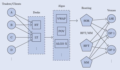
In first instance, one might separate traders into two groups – those trading with proprietary access to exchanges, and those trading through execution services/brokers. The first group primarily contains high-frequency traders and market makers. Note, that most market makers (MMs) are also high-frequency traders. Nonetheless, we distinguish between these as MMs have a particular, liquidity-providing function. The remainder are traders which trade through execution services and are not in full control of the actual placement of limit orders. These traders, depicted on the left side, send parent orders (also called meta orders) to a particular desk of a broker. The broker then uses scheduling algorithms, such as VWAP, TWAP, POV to slice the parent order into a stream of child orders according to the trader's preferences. The resulting child orders are then sent as limit or market orders to different venues via a smart order router (SOR). Some of these venues may be lit venues, such as XETRA or LSE exchange, others could be, for example, dark pools or other systematic internalizers. Studies using public LOB data only see what is being sent to exchanges at the end of the order process (right hand-side of figure 1).

This heterogeneity, which is arguably an important feature for risk managers and market regulators (Kirilenko et al. 2017), is challenging to model. Indeed, most stochastic models proposed for limit order book dynamics (Smith et al. 2003, Cont et al. 2010) represent the order flow as a homogeneous point process, often for reasons of analytical tractability. These models are generally based on aggregate order flow data such as the LOBSTER database¹ , which does not contain information on parent orders or agents submitting them.

Our contributions are twofold. First, we introduce a new granular representation of the limit order book which accounts for the origin of orders and distinguish different levels of information such as the anonymized view, which has been the focus of previous studies, from the broker view which is the focus of our analysis.

Second, using detailed order flow data from a major broker, we investigate the structure of the incoming order flow (e.g. the left side of figure 1. We use trade execution data to segment traders into representative groups with similar attributes. These are then analyzed for stability in both the cross-sectional (i.e, cross-asset) and temporal dimensions. To the best of our knowledge, our study is the first one to provide an analysis of a broker's parent order flow.

We find that equity order flow can be segmented into four different components: Quant, Day VWAP, Signal and Res(residual) order flows. The different groups are stable both over time as well as across stocks. This also holds for the traders themselves. Heterogeneity in both the agents' structure and the order flow they generate in LOBs allows the development of heterogeneous order flow models.

Based on these results, we present a modeling framework for client order flow from the viewpoint of a broker. Without going down to the level of granularity of an agent-based model, our framework decomposes the order flow into components representing different agent types, while remaining easy to calibrate and simulate.

Outline. Section 2 introduces a granular representation of the LOB accounting for the origins of orders, which allows for different views on the LOB. Section 3 presents the data on client order flow and describes its segmentation into different components, which we identify as representative agent types. Section 4 describes the properties of the order flow for each agent type. A simple model for parent order flow capturing the main heterogeneity between the different agent types is presented in Section 5. Section 6 summarizes the results and presents future research directions.

1.1. Related work

There exists a vast literature on the statistical properties and stochastic modeling of limit order books, using public data; some references may be found in Bouchaud et al. (2002), Cont (2011), and Gould et al. (2013).

Smith et al. (2003), Cont et al. (2010), and Cont and De Larrard (2013) model the LOB via Poisson point processes. Sirignano and Cont (2019) and Zhang et al. (2019) use deep learning for short-term prediction of price moves. Agent-based models have also been proposed for LOBs (Byrd et al. 2019, Vyetrenko et al. 2019), but such models struggle with calibration since it is not clear how to calibrate parameters governing agent behavior in the absence of agent-level order information.

There are fewer studies on order flow characteristics of particular types of market participants, due to the confidential nature of such data. Brogaard (2010) and Brogaard et al. (2014) study LOB data in which orders from HFTs and MMs are flagged, in order to analyze the impact of HFT and MM accounts on market quality and price discovery. The studies find evidence that HFTs increase market quality by potentially dampening intraday volatility among other properties. Furthermore, they argue that the trade directions of HFTs are based on public information such as ‘macro news announcements, market-wide price movements, and limit order book imbalances’ Brogaard et al. (2014). Hagströmer and Nordén (2013) analyze LOB data with information about orders from HFTs and MMs, specifically outlining the differences between these two types of market participants in the way they tend to trade. They find MMs to take the majority of limit order traffic and to hold lower inventories compared to HFTs. Along these lines, Van Kervel and Menkveld (2019) investigate the behavior of HFTs when large institutional orders are being executed. Hasbrouck and Saar (2013) attempt to extract HFT trades by identifying the so-called ‘strategy runs’, i.e. periods with similar inter-arrival times and order sizes, which is unique for HFTs, as the authors argue. Their suggested measure of low latency indicates that with increasing low latency trading, spreads decrease and the depth at the first level increases.

The information content of broker order flow has been studied by Barbon et al. (2019), Di Maggio et al. (2019) and Hendershott et al. (2020). Hendershott et al. (2020) analyze transaction costs in over-the-counter corporate bonds markets, depending on the network size of the insurers. Di Maggio et al. (2019) analyze non-public data to study the network of links between institutional investors and brokers. Barbon et al. (2019) use similar data focusing on large liquidations of funds, finding that clients of brokers which are aware of such large liquidations tend to execute much more during such events.

A related study is Kirilenko et al. (2017)'s analysis on transactions in S&P 500 E-Mini futures during the Flash Crash of May 2010 using audit trail data. Kirilenko et al. (2017) classify the agents into high-frequency traders, market makers, fundamental buyers, fundamental sellers and opportunistic traders, based on transaction volume and scaled net positions. Despite having access to a very granular data set, the analysis is focused on high-frequency traders and market makers during the flash crash, and less on the properties of the remaining market participants.

Our analysis is broader and focused on multiple tickers across a longer period, using a more detailed data set containing information on parent orders and order flow as well as transactions. In particular we are able to include order flow from traders who do not have direct market access to the exchanges.

2. The limit order book as a heterogeneous queuing system

We consider a set of agents A, representing different traders or agent types submitting orders to a limit order book.

Definition 2.1

A limit order (LO) $x=(t,p,q,\alpha )$ is characterized by

• an arrival time $t\in {\mathbb{R}}^{\mathbb{+}}$,

• a price $p\in \delta \mathbb{N}$ which is a multiple of the price tick $\delta >0$,

• a quantity $q\in \mathbb{Z}\setminus \left\{0\right\}$ with q<0 denoting buy orders and q>0 denoting sell orders,

• the identity $\alpha \in A$ of the agent submitting the order.

A limit order is considered ‘outstanding’ as long as it has neither been cancelled nor fully executed.

A market order is an order for immediate execution. We represent market orders as an executable limit order with price p = 0 (for a market buy order) or $p=\mathrm{\infty }$ (for a market sell order).

If an order is cancelled, it is removed from the LOB. Alternatively, when a partial cancellation occurs, the order size q is decreased.

Denote by ${ϵ}_x$ the unit point mass at x by and by ${\mathcal{M}}_{+}({\mathbb{R}}_{+}\times \delta \mathbb{N}\times A),$ the space of (Radon) measures on ${\mathbb{R}}_{+}\times \delta \mathbb{N}\times A$. and One can represent the collection of buy (resp. sell) orders as a pair of measures ${\mu }_{+},{\mu }_{-}\in {\mathcal{M}}_{+}({\mathbb{R}}_{+}\times \delta \mathbb{N}\times A)$ where ${\mu }_{+}\left(\right[0,t]\times \{p\}\times \{\alpha \left\}\right)$ (resp. ${\mu }_{-}\left(\right[0,t]\times \{p\}\times \{\alpha \left\}\right)$ ) represents the volume of buy (resp. sell) orders submitted by agent α at price p, between time 0 and t.

The order book may then be represented as a signed measure (1) $\mu ={\mu }^{+}-{\mu }^{-}.$(1)

2.1. Anonymized view

The anonymized or aggregate view of the limit order book corresponds to the information available to market participants who observe the volume of orders at each price. It does not contain any information regarding the origin nor the submission times of the orders. Hence, most market participants only observe the queue size $Q_p$ at each price level p

Definition 2.2

The queue size for any price $p\in \delta \mathbb{N}$ is denoted by (2) $Q_p=\sum _{\alpha \in A}\mu \left(\right[0,t],\{p\},\alpha ).$(2) We call $Q:\delta \mathbb{N}\to \mathbb{Z}$ the anonymized limit order book, $Q\in \mathcal{M}\left(\delta \mathbb{N}\right)$ and belongs to the state space ${\mathbb{Z}}^{\delta \mathbb{N}}$. Note, for the anonymized view, t must generally correspond to the current time. In other words, market participants with access to the anonymized view at time t are not able to access the net volume of those outstanding orders that have been submitted in $[0,t^{\prime }]$, with $t^{\prime }<t$. This would reveal information about the queue position, which generic market participants generally do not have. In case exchanges offer detailed event-to-event flow with, in particular, cancellations referring to particular orders, tracking the queue position is possible.

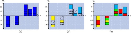
The anonymized view is visualized in figure 2(a) and corresponds to the sum of all orders' quantity at a particular level. The agent neither observes the number of orders nor the color (i.e. the agent id).

Figure 2. Different views of the same LOB snapshot. Note, only the omniscient view has complete information about the queue priority of each order. (a) anonymized view (b) Broker view (c) Omniscient view.

2.2. Omniscient view

The omniscient view of the limit order book is the collection of all outstanding limit orders, including the information about their time of submission and the identity of the submitter. This information is represented by the measure μ. E.g. in figure 2(c), the omniscient view not only contains the single orders with prices and quantities, but also the color (i.e. the agent id). Outstanding orders from agent $\alpha \in A$ are then represented by (3) $\mu (\cdot ,\cdot ,\{\alpha \left\}\right)\in {\mathcal{M}}_{+}({\mathbb{R}}_{+}\times \delta \mathbb{N}).$(3)

2.3. Broker view

The omniscient view and the anonymized limit order book represent two extreme cases of information on the limit order book. However, there are intermediate situations corresponding to partial information on the limit order book. An important case is the case of a broker who can observe the order submission times and identities for a subset $B\subset A$ of agents. This broker will have a less detailed view of the limit order book, which corresponds to aggregating over all agents not in B. Denote by $B^{\ast }=B\cup \left\{\mathrm{\Delta }\right\}$ the set obtained by adding one element to B; this element will represent all other agents not included in the broker's set of clients. The broker view of the limit order book may then be described by a measure ${\mu }_B\in \mathcal{M}({\mathbb{R}}_{+}\times \delta \mathbb{N}\times B^{\ast })$ defined by (4) $\begin{array}{rl}{\mu }_B(\cdot ,\cdot ,\{\alpha \left\}\right)& =\mu (\cdot ,\cdot ,\{\alpha \left\}\right)\alpha \in B,\end{array}$(4) (5) $\begin{array}{rl}{\mu }_B(\cdot ,\cdot ,\{\mathrm{\Delta }\left\}\right)& =\sum _{\alpha \notin B}\mu (\cdot ,\cdot ,\{\alpha \left\}\right).\end{array}$(5) An exemplary broker view snapshot is visualized in figure 2(b) next to the public and omniscient view of the same snapshot. Yellow and light blue correspond to agents $\alpha \in B$ thus are from the broker's clients. These orders are observed with their particular ID and viewed via ${\mu }_B(.,.,\{\alpha \left\}\right)$, while green and red orders would correspond to ‘all other agents’ (Δ) which are not in B, the broker's set of clients. These orders are seen as ${\mu }_B(.,.,\{\mathrm{\Delta }\left\}\right)$. Furthermore, the broker does not observe the specific time as (5(5) $\begin{array}{rl}{\mu }_B(\cdot ,\cdot ,\{\mathrm{\Delta }\left\}\right)& =\sum _{\alpha \notin B}\mu (\cdot ,\cdot ,\{\alpha \left\}\right).\end{array}$(5) ) suggests, but rather the relative time since the broker knows its queue position. Hence, the broker can (only) know that an order has been submitted between two orders of its own clients.

Most literature aims to model the anonymized view of the LOB. These models have been shown to be useful for describing certain dynamics of limit order books. They include general price moves or distribution of queue sizes. The detailed queue and a specific order's queue position, however, is generally not available in both public data and the majority of the models in the literature. This has led to research aiming to estimate the queue position of an order (Moallemi and Yuan 2016). As shown by Moallemi and Yuan (2016), ‘queueing effects can be very significant’ and accounting for the queue position should not be ignored when designing trading algorithms. In accordance to this, keeping track of the queue size rather than the entire collection of orders does not allow cancellations to refer to particular orders. This makes keeping track of how orders flow through the queue impossible. Instead, a LOB model which accounts for this heterogeneity allows to do this. We remark that the topic of identifying determinants of limit order cancellations has been extensively studied recently and would be an interesting research direction to explore, in itself.

As figure 1 visualizes, limit orders sent through a broker part of a larger parent order. Since these parent orders are central in the sequel of the paper, we formally introduce the structure of a parent order.

Definition 2.3

A parent order P is defined by a number of variables some of which are determined by the submitting trader, others are only known at the end of the execution.

• a submission or arrival time $t\in {\mathbb{R}}^{+}$,

• a target quantity $q^{target}\in \mathbb{Z}\setminus \left\{0\right\}$, the total quantity which shall be executed in the market,

• an executed quantity $q^{exec}\in \mathbb{Z}$ which corresponds to the total sum of executed child orders.

The parent order's target quantity $q^{target}$ can be decomposed in its absolute quantity $\tilde{q}=\left|q^{target}\right|\in \mathbb{N}$ and sign (buy or sell order) (6) $\mathrm{s}\mathrm{i}\mathrm{g}\mathrm{n}\left(q^{target}\right)=\{\begin{array}{ll}-1,& if{q}^{target}<0\\ 1,& if{q}^{target}>0.\end{array}$(6) Each order has an order placement schedule, which we denote by (7) $\mathcal{X}=\{x_1,\dots ,x_N\},x_i=(t_i,p_i,q_i,{\alpha }_i)\mathrm{\forall }{x}_i\in \mathcal{X},$(7) where each element has the form of a LO as defined in Definition 2.1. The schedule contains all LOs placed within the parent order execution. Hence, ${\alpha }_i=\alpha$ since all limit orders are posted by the same agent. Note, $\mathcal{X}$ may contain effective market orders as executable limit orders. As mentioned above, a buy limit order ($q_i<0$ with price $p_i=\mathrm{\infty }$) would correspond to a buy market order ($q_i>0$ and $p_i=0$ to a sell market order, respectively).

Additionally, there is an execution schedule (8) $\begin{array}{r}{\mathcal{X}}^{exec}=\{x_1,\dots ,x_N\},x_i=(t_i,p_i,q_i,{\alpha }_i)\mathrm{\forall }{x}_i\in {\mathcal{X}}^{exec},\end{array}$(8) which is comprised of all market orders affecting the parent order P. This can either be a market order x with $p\in \{0,\mathrm{\infty }\}$ sent within the order schedule in equation (7(7) $\mathcal{X}=\{x_1,\dots ,x_N\},x_i=(t_i,p_i,q_i,{\alpha }_i)\mathrm{\forall }{x}_i\in \mathcal{X},$(7) ); in this case, $x\in \mathcal{X}$. Or, a market order x is sent by any other agent which (partially) executes an outstanding order from $\mathcal{X}$; in this case, $x\in {\mathcal{X}}^{exec}$ but $x\notin \mathcal{X}$.

Note, any element $x\in {\mathcal{X}}^{exec}$ from another agent ${\alpha }^{\prime }$ may not be the complete market order. Assume an incoming market order executes several limit orders. In this case, only the fraction affecting a limit order in $\mathcal{X}$ is kept in ${\mathcal{X}}^{exec}$. If two limit orders of $\mathcal{X}$ are executed by the same market order, then there are two entries with the same time stamp. Alternatively, several market orders affect a limit order from $\mathcal{X}$ currently outstanding. In this case, there are also several elements in ${\mathcal{X}}^{exec}$, one for each partial execution of an order in $\mathcal{X}$. Note, both the limit order schedule as well as the execution schedule are only fixed after execution.

A full description of the market, the omniscient view, is not always available. The broker view, however, offers a partially more detailed view on the market, in particular, of the broker's set of agents B. Thus, we want to shed some light into what B consists of to better understand the limit order market ecosystem. In case, the ecosystem can be separated into several groups of order flows, modeling the order flow of each group is a much more feasible and tractable task in comparison to modeling every single agent $\alpha \in B$. Thus, the remainder of this paper analyses the order flow of a broker and separates a typical set of agents using execution services into different representative groups. These show homogeneous behavior within their group but differ substantially across different groups.

3. Segmentation of agent types

This section considers the task of segmenting the population of traders that send orders to the brokers. Traders sending orders build the very left hand side of figure 1. Our analysis of this process stands in contrast to known works in the literature, since most studies only use anonymized order flow data, as outlined in section 1.1. Few studies use non-public LOB data, and mainly Kirilenko et al. (2017) have access to the trading accounts. Consequently, the available data structure not only allows us to observe what arrives in the LOB and who sends it, but also whether several limit orders come from the same parent order. Uncovering latent similarities across traders and identifying different trader typologies can potentially facilitate better modeling of the parent order flow in LOBs. The main implication of our findings is that one can move beyond modeling each agent or trader independently and pave the way for modeling each homogeneous group or cluster of agents.

3.1. Data set and features

For the analysis, we use anonymized trade execution data from a major broker. Market shares can be found in reports from industry providers of strategic benchmarking such as Coalition. The data used in this paper forms a market share mostly in the high single-digit percentage – depending on the stock. This makes it amongst the largest private data sets of broker execution data in European markets. This gives reason to assume that the results are unlikely to be completely different at other large brokers. The motivation for this stems from the fact that traders often do not only trade solely via one broker but via several major brokers. This data set builds a detailed view on a subset of the entire market, as explained in the previous sections. In particular, it allows one to observe what traders submit to the broker as a parent order, up to where and when different child orders corresponding to this parent order are placed. This holds for both lit and dark venues. The universe is comprised of stocks from STOXX 600, and buckets of 1-month duration will be employed in the segmentation.

For each asset i and time period t, the set of traders that execute their trades via the broker is denoted as $B_{i,t}$ where each agent $\alpha \in B_{i,t}$ has sent at least one order to the broker which led to an execution. Clearly, $B_{i,t}\subseteq A_{i,t}$, the whole set of agents active in a LOB of the given ticker. Instruments are primarily analyzed separately; joint analysis is used primarily for matters of comparison and stability, in particular in section 3.4.

Generally speaking, the broker manages the execution and the child orders which are sent to the LOB. For the analysis, we thus rely on the parent order structure and the corresponding statistics for each agent. Features regarding the single-child orders are not included. This means: when do agents send orders, how large are they, and how aggressive shall they be executed? The corresponding data fields are primarily side (buy/sell), number of orders, time of submission and size. The resulting features/statistics of this information include, for example, the average direction of an agent's trades, the number of orders an agent has submitted, distributional properties of the day time an agent submits orders, or an agent's order sizes' standard deviation. Information regarding external information or market conditions such as momentum, volatility, etc. are also used. A detailed description of each feature can be found in table A1.

Altogether, this amounts to a data set of $n=\left|B_{i,t}\right|$ agents with p features $X\in {\mathbb{R}}^{n\times p}\text{ with }{x}_{\alpha }=(x_{\alpha ,1},\dots ,x_{\alpha ,p})\in {\mathbb{R}}^p\mathrm{\forall }\alpha \in B_{i,t}$ describing $B_{i,t}$. Each vector $x_{\alpha }$ describes the parent order structure of agent α in instrument i during period t. The data sets, and in particular the various features considered, are of different dimensions and also ranges. Furthermore, some features are heavily skewed, having many smaller values and few very large values. This holds true in particular for features like order size or number of orders. Thus, we use the logarithm of such features and then standardize the data before proceeding with any further analysis. To this end, we apply z-standardization using the sample mean and standard deviation. Alternatively, methods like min-max normalization may be used. In the present case, no major differences could be noted using different normalization techniques.

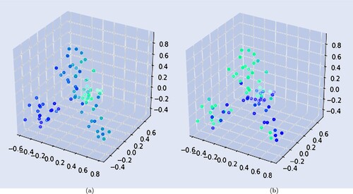
To visualize agents in a lower-dimensional space and get a first idea of the data structure, methods such as principal component analysis (Hastie et al. 2009) or spectral embedding (Belkin and Niyogi 2002) may be applied to obtain further insights into the structure of the agents interacting with financial brokers. To this end, figure 3 shows two exemplary features in the embedding space. The mean creation time of a client's orders in figure 3(a) and the ratio indicating the fraction of orders of a particular trader which contains a maximum price for the execution (minimum price for sell orders, respectively) in figure 3(b). For both features in figure 3, there are areas of the embedding where traders with similar values of the corresponding features are clustered. For example, there exists an area of traders which have much higher mean creation time compared to that of other clusters. In figure 3(b), a group of traders can be encountered which tends to specify a limit price when sending orders for executions. Additionally, the fact that the point cloud in the embedding is not just a sphere indicates some structure in the underlying data which can be further exploited.

Figure 3. Exemplary embedding using the first three eigenvectors of the normalized Laplacian matrix using the spectral embedding method from Belkin and Niyogi (2002). The color of the nodes indicates the values of the associated feature. The brighter the points, the higher the value of the corresponding feature. (a) Mean creation time (b) Ratio of specified limit price.

3.2. Spectral clustering

As outlined in section 2, a broker has a detailed view on a subset of the market, i.e. knows the trader identity and the specific time of an order, for all agents $\alpha \in B_{i,t}$. For ease of notation, we will refer to $B_{i,t}$ as B in the sequel. To better understand the structure of a typical set of traders which use a broker, this section segments B into a disjoint partition $\mathcal{C}=\{C_1,\dots ,C_K\}$, in order to obtain representative agent types that best describe the structure of a broker's clients.

Clustering algorithms are designed to do exactly what is this section's purpose. They separate the observations into different, typically unknown, classes or clusters. These types/clusters should be heterogeneous, but traders of the same type should rather form a homogeneous population with similar characteristics. Referring to figure 1, we would like to shrink down the number of nodes representing many individual traders submitting parent orders on the left hand side to just a few nodes representing each trader type. K indicates the number of types the agents shall be separated into. ${\overline{x}}_1,\dots ,{\overline{x}}_K\in {\mathbb{R}}^p$ are the corresponding cluster centers indicating the average features (i.e. coordinates) of the data points (i.e. agents) affiliated with the corresponding cluster, so ${\overline{x}}_{k,j}=\frac{1}{\left|C_k\right|}\sum _{\alpha \in C_k}{x}_{\alpha ,j}\mathrm{\forall }j\in \{1,\dots ,p\}$. Essential to each clustering algorithm is a distance matrix $W\in {\mathbb{R}}^{n\times n}$ which contains the distance $W_{\alpha ,{\alpha }^{\prime }}$ between observation $x_{\alpha }$ and $x_{{\alpha }^{\prime }}$, for some distance measure d. This distance is often the Euclidean distance.

The spectral clustering technique used in this study combines two methods, spectral embedding and the K-means clustering algorithm (Shi and Malik 2000, Meila and Shi 2001, Ng et al. 2002). In other words, it creates the partition via an iterative ascent algorithm on a $p^{\prime }$-dimensional, non-linear embedding of the data set, describing the agents' trading behavior.

1. Construction of the adjacency graph

   The adjacency graph indicates for each pair of observations whether these are connected or not. In particular, (9) $\begin{array}{rl}A& \in {\mathbb{R}}^{n\times n}\text{ where }{A}_{i,j}\\ & =\{\begin{array}{ll}1& \mathrm{i}\mathrm{f}\Vert x_i-x_j{\Vert }^2<ϵ\\ 0& \mathrm{e}\mathrm{l}\mathrm{s}\mathrm{e},\end{array}\mathrm{\forall }i,j\in \{1,\dots ,n\}.\end{array}$(9) Two vertices are connected by an edge if their Euclidean distance in the actual space ${\mathbb{R}}^p$ is below a certain threshold ϵ. Alternatively, one may connect a vertex i to its l nearest neighbors where $l\le n,l\in \mathbb{N}$.

2. Weighting the similarities

   This step weighs the connections between observation i (row) and j (column). The common choice is the heat/rbf kernel. In this case, the matrix $W\in {\mathbb{R}}^{n\times n}$ is computed with (10) $W_{i,j}=\{\begin{array}{ll}{e}^{-\frac{\Vert x_i-x_j{\Vert }^2}{\sigma }}& \mathrm{i}\mathrm{f}{A}_{i,j}=1\\ 0& \mathrm{e}\mathrm{l}\mathrm{s}\mathrm{e}\end{array}\mathrm{\forall }i,j\in \{1,\dots ,n\},$(10) for some user-tuned bandwidth parameter $\sigma \in {\mathbb{R}}_{+}$. The closer (i.e. more similar) the observations $x_i$ and $x_j$ are in Euclidean distance, the higher the value $W_{ij}$. Alternatively, whenever the input matrix is binary, with $A_{i,j}=1$ for connected vertices, we set $W_{i,j}=1$ if $A_{i,j}=1$.

3. Compute eigenmaps via first $p^{\prime }$ eigenvectors

   Next, the generalised eigenvector problem (11) $Lf=\lambda Df,$(11) is solved. $D\in {\mathbb{R}}^{n\times n}$ is a diagonal matrix containing the row-sums of W, i.e. $D_{i,i}=\sum _j{W}_{i,j}$. We define L = D−W to be the unnormalized Laplacian matrix (also referred to as the Combinatorial Laplacian).

   The solution of equation (11(11) $Lf=\lambda Df,$(11) ) is a set of (sorted) eigenvalues $\lambda =({\lambda }_0,\dots ,{\lambda }_{n-1})$ for which ${\lambda }_0\le {\lambda }_1\le \cdots \le {\lambda }_{n-1}$ holds. For the corresponding eigenvectors $f=(f_0,\dots ,f_{n-1})$ from equation (11(11) $Lf=\lambda Df,$(11) ) ${\lambda }_0=0$ and $f_0=(1,\dots ,1)\in {\mathbb{R}}^n$ holds Von Luxburg (2007). The multiplicity of the ${\lambda }_0=0$ indicates the number of connected components in the graph. Finally, the eigenvectors $f_1,\dots f_{p^{\prime }}$ are then used for the $p^{\prime }$-dimensional embedding and $y_i=\left(f_1\right(i),\dots ,f_{p^{\prime }}(i\left)\right)\in {\mathbb{R}}^{p^{\prime }}$.

4. Clustering the low-dimensional embedding

   Finally, the agents are clustered in this low-dimensional embedding via the K-means algorithm MacQueen (1967). The objective function optimized by the algorithm is given by (12) $\underset{\mathcal{C},\{{\overline{y}}_k{\}}_k}{min}\sum _{k=1}^K\left|C_k\right|\sum _{\alpha \in C_k}\Vert y_{\alpha }-{\overline{y}}_k{\Vert }^2,$(12) where $y_{\alpha },{\overline{y}}_k\in {\mathbb{R}}^{p^{\prime }}$, the space of the embedding. The objective function (12(12) $\underset{\mathcal{C},\{{\overline{y}}_k{\}}_k}{min}\sum _{k=1}^K\left|C_k\right|\sum _{\alpha \in C_k}\Vert y_{\alpha }-{\overline{y}}_k{\Vert }^2,$(12) ) corresponds to the minimization of the variance within the clusters with respect to partition $\mathcal{C}$. Optimization is done via iterative descent, alternating between recomputing cluster centers ${\overline{y}}_k$ and reassigning the observations $y_{\alpha }$ to the nearest cluster center² .

In contrast to K-Means, spectral clustering is a non-linear clustering method. This enables the algorithm to potentially uncover clusters that are not convex since the clustering is not performed in the original feature space ${\mathbb{R}}^p$, but rather in the embedding space ${\mathbb{R}}^{p^{\prime }}$ (Von Luxburg 2007). This capability of uncovering non-linear relationships makes spectral clustering more flexible in comparison to K-Means.

Extracting centroids of a partition when using spectral clustering is not as straight forward as for K-Means. This is because the embedding procedure described above is not invertible for any arbitrary point. Hence, a point $y\in {\mathbb{R}}^k$ cannot be mapped into the actual feature space ${\mathbb{R}}^p$. To overcome this, one can use the center of a cluster's observations in the actual space from the data $X\in {\mathbb{R}}^{n\times p}$, i.e. ${\overline{x}}_k=\frac{1}{\left|C_k\right|}\sum _{i\in C_k}{x}_i\mathrm{\forall }k\in \{1,\dots ,K\}$. Alternatively, the prototype for cluster k can be defined as $x_i\in {\mathbb{R}}^p\mathrm{w}\mathrm{i}\mathrm{t}\mathrm{h}i=\underset{i\in C_k}{\mathrm{a}\mathrm{r}\mathrm{g}\mathrm{m}\mathrm{i}\mathrm{n}}\Vert y_i-{\overline{y}}_k{\Vert }^2$. In other words, the observation $x_i$ is the one whose embedding $y_i$ is the closest to the cluster center ${\overline{y}}_k$ in the embedding space. In this study, the first method is used to obtain cluster centers, as it is less prone to outliers for some features of the prototype $x_i$. The cluster centers are then used to give details about properties and provide a comparison of the different agent types.

Several algorithms were used to cluster $B_{i,t}$ and find an optimal partition $\mathcal{C}$. In the following, we particularly outline observations and statistics when comparing the partitions between K-means and spectral clustering in more detail for one exemplary $B_{i,t}$. The number of clusters K ranges from 2 to 5. The number of agents for the ticker is $\sim 80$.

Cluster sizes: Generally, the number of observations in the clusters is neither very large nor very small. There is no cluster with only very few observations.

Consistency: The partitions using K-means and spectral clustering are very similar. This consistency can be quantified by the adjusted rand index (ARI) which indicates the consistency across two partitions. Let ${\mathcal{C}}^{\left(1\right)}=\{C_1^{\left(1\right)},\dots C_K^{\left(1\right)}\}$ and ${\mathcal{C}}^{\left(2\right)}=\{C_1^{\left(2\right)},\dots C_K^{\left(2\right)}\}$ be two partitions. The ARI reads (13) $ARI=\frac{\sum _{k,k^{\prime }}(\genfrac{}{}{0ex}{}{n_{k,k^{\prime }}}{2})-\left[\sum _k(\genfrac{}{}{0ex}{}{a_k}{2})\sum _{k^{\prime }}(\genfrac{}{}{0ex}{}{b_{k^{\prime }}}{2})\right]/(\genfrac{}{}{0ex}{}{n}{2})}{\frac{1}{2}[\sum _k(\genfrac{}{}{0ex}{}{a_k}{2})+\sum _{k^{\prime }}(\genfrac{}{}{0ex}{}{b_{k^{\prime }}}{2})]-\left[\sum _k(\genfrac{}{}{0ex}{}{a_k}{2})\sum _{k^{\prime }}(\genfrac{}{}{0ex}{}{b_{k^{\prime }}}{2})\right]/(\genfrac{}{}{0ex}{}{n}{2})},$(13) where $n_{k,k^{\prime }}=|C_k^{\left(1\right)}\cap C_{k^{\prime }}^{\left(2\right)}|$ denotes the number of observations inside $C_k^{\left(1\right)}$ and $C_{k^{\prime }}^{\left(2\right)}$ and $a_k=\sum _j{n}_{k,k^{\prime }}=\left|C_k^{\left(1\right)}\right|$ ($b_{k^{\prime }}=\sum _k{n}_{k,k^{\prime }}=\left|C_{k^{\prime }}^{\left(2\right)}\right|$). The index takes a maximum value of 1 if ${\mathcal{C}}^{\left(1\right)}={\mathcal{C}}^{\left(2\right)}$.

Table 1 shows the ARI for different values of K. A particularly high consistency is indicated for 2 and 4 clusters. Noteworthy is the high consistency taking into account that K-means is performed on the actual feature space (${\mathbb{R}}^p$), while the spectral clustering is based on the non-linear embedding in ${\mathbb{R}}^{p^{\prime }},p^{\prime }\ll p$. In other words, regardless of the feature space employed, the recovered partitions are very similar.

Table 1. Table indicating the ARI between K-means and spectral clustering.

# Clusters	2	3	4	5
ARI	0.7979	0.5107	0.7968	0.6153

Note: The higher the number, the higher the consistency between to partitions; the maximum value ARI can attain is 1, indicating a perfect matching of the clusters.

Stability of clusters: Increasing K leads to a sequential splitting of the data cloud into clusters. E.g. one cluster gets further split when increasing K by one unit. The other clusters and their affiliated traders remain stable.

Number of clusters: Setting K = 2 or K = 4 leads to the best scores. First of all, the consistency is better than for 3 and 5 clusters indicated by higher ARIs in table 1. Lastly, table 2 shows the variance between agents and their corresponding cluster center. In particular, the more the variance decreases, the more justified is the addition of another cluster. The second differences of the variance within the clusters can indicate how the variance reduction of an additional new cluster changes. This helps to identify a K, for which an increase leads to a much lower variance reduction. In particular, values for K would be either 2 or 4, which goes in line with the other metrics.

Table 2. The variance between an observation and its corresponding cluster.

# Clusters	1	2	3	4	5	6	7	8	9
Variances	3.914	3.507	3.210	2.981	2.871	2.738	2.640	2.596	2.536
2nd Diffs.	–	0.108	0.069	0.118	−0.021	0.034	0.053	−0.016	–

Note: The stronger the decrease when K is increased by one cluster, the larger is the marginal effect of the new cluster to separate the data.

3.3. Representative agent types

Despite the final goal being the heterogeneity of the aggregated order flow caused by different clusters, the cluster centers ${\overline{x}}_k=\frac{1}{\left|C_k\right|}\sum _{i\in C_k}{x}_i$ are computed to interpret the agent types. Such resulting cluster centers for a subset of the features used are shown in table 3, for one exemplary $B_{i,t}$.

Table 3. Exemplary centroids setting K = 4 for one of the 25 most liquid STOXX 600 instruments during December 2019.

	1: Quant	2: Day VWAP	3: Signal	4: Res
Buy ratio	0.63	0.55	0.63	0.65
Cancellation ratio	0.26	0	0.15	0.07
# Trades per month	219.7	1.72	4.08	5.03
Maximum order creation time	16:10:47	08:32:04	15:02:03	14:34:05
Mean order creation time	12:03:50	08:25:34	14:20:00	11:31:56
Mean order size (in ADV)	0.01	0.03	0.06	0.06
Mean momentum (bps)	2.285	−17.87	29.94	38.26
Mean volatility	22.2	23.03	22.42	22
Minimum order creation time	07:58:08	08:19:10	13:34:31	08:40:12
# Active days per month	13.47	2.1	3.71	4.95
St. dev. of order creation time	02:24:49	00:07:12	00:42:16	02:40:46

Notes: Liquidity, in this case, refers to the total number of trades in the data base. The highest (lowest) value of the corresponding features are highlighted in bold (italics).

In fact, as shown in table 4, the four agent types may be summarised as follows:

1. Quantitative agents (Quant): The most distinguishable agent type is cluster 1, which contains those agents that submit many trades within the period, with a smaller trade size. Despite trading rather small amounts, the total volume traded is by far the highest in this cluster. Also, the number of days during which the cluster's agents trade is 12 days, which is several times higher than the second highest value. Cluster 1 exhibits the highest average cancellation rate, indicating that this agent type perhaps tracks the execution of its trades more actively than other types. Also, the day time of the trades is uniformly distributed across the whole day, with a mean creation time around noon. This type of agent may be summarised as a ‘quantitative agent’, called Quant in the following sections.

2. Day VWAP agents (Day VWAP): The most distinct cluster from Quant is cluster 2 as its features exhibit the largest anti-correlation to features of Quant. The number of trades per agent is the lowest, and all trades are submitted very early in the morning. The average trade size is larger than for Quant, yet not the largest across the agents for this partition. Most noticeable apart from the few number of trades with larger size is the creation time of the order, which typically only occurs before market open. This indicates that these orders are large orders typically sent before market opening, and with an execution target over the entire day. Looking at the execution algorithm, one can primarily find rather passive algorithms such as VWAP, which further support the previous statement. This trading behavior is further reflected in the cancellation rate, which is the lowest across all clusters, while having most child orders during the execution. This type of agent is summarised as a ‘Day VWAP agent’, called Day VWAP in the following sections.

3. Signal agents (Signal): Cluster number 3 is most distinguishable due to its creation time, which shows a minimum of ∼ 13:30 and a maximum of ∼ 15:00 for the corresponding data slice. Hence, this is an agent type which is typically active in the afternoon (which corresponds to the opening of the US market since it is a STOXX 600 instrument). Similar to Day VWAP, the cancellation rate is quite small, only $\sim 5\mathrm{\%}$, when compared to Quant which is around $\sim 14\mathrm{\%}$. This agent type tends to execute large order sizes ($5\mathrm{\%}$ of the average daily volume of the last 20 days). Additionally, the cluster in this example has a high percentage of volume, and significant fractions are executed via dark venues which leads us to assume the agent type is less concerned about execution costs but has a high urgency – hence also executes a lot in dark venues to mitigate traces in the market. The reason may be that this agent type wants to act on trading signals and is thus referred to as a ‘Signal agent’, called Signal in the following sections.

4. Residual agents (Res): Cluster 4 indicates agents with the largest average trade size, and only about five trades per month. The trades are submitted during the entire day, which is also indicated by the high standard deviation of the creation time. Furthermore, the standard deviation of the sizes, as measured in the logarithm of the average daily volume percentage, is the highest. This is the ‘least distinguishable’ agent type, and seems to be in-between the other three clusters. One possible reason may be that some agents trade different strategies and thus do not act very homogeneously. Hence, these agents may be referred to as ‘residual agent’, denoted as Res in the following sections.

Table 4. Summary of agent types.

Cluster Name	Cluster Description
Quant	Mainly quantitative traders, many trades, small volumes, orders sent throughout the day, execution with few child orders leading to a large POV, net inventory closer to 0
Day VWAP	Mostly VWAP as execution, few orders, only sent in the morning, almost no cancellation
Signal	Typically trading in the afternoon (especially US market opening), large trades, large amount traded in dark venues, large POV in general
Res	Large orders, medium frequency, sent throughout the day

3.4. Stability of clusters

Section 3.3 shows that the set of agents $B_{i,t}$, trading asset i during period t through a broker, can be segmented into different clusters. Setting K = 4 gives an appropriate number of agent types which can be interpreted and are also very distinct in their representative features. Moreover, the partitions do not change significantly when changing the clustering algorithm or the feature standardization procedure.

It is, however, unknown how the cluster affiliations and the representative agent types change over time or different instruments. Are the results in section 3.3 random or is the partition rather stable? This section addresses the stability of the agents and clusters, both across different instruments as well as different time slices. One problem arising when comparing two partitions in the present case is that most often $B_{i,t}\ne B_{j,t^{\prime }}$. In other words, traders which are active in asset i during period t do not necessarily trade asset j during period $t^{\prime }$. Nonetheless, the following two questions are of particular interest. First, how stable is the affiliation of an agent to a particular cluster? Do agents change their behavior and act differently across time or different tickers? Second, how stable are the agent types and their features presented in section 3.3?

Two approaches are pursued to answer these questions:

1. Joint clustering of several data slices:

   As before, $B_{i,t}$ is the set of agents α with at least one trade in asset i during period t. For example, ${\overline{x}}_{i,\alpha }=\frac{1}{\left|T_{i,\alpha }\right|}\sum _{t\in T_{i,\alpha }}{x}_{i,t,\alpha }$ (where $T_{i,\alpha }=\left\{t\right|\alpha \in B_{i,t}\}$) denotes the average of a trader's features across all time periods in which they have traded at least once. If T periods of one asset i, i.e. $B_{i,t}\mathrm{\forall }t\in \{1,\dots ,T\}$ are clustered together, a high concentration of observations from one agent, e.g. $x_{i,t,\alpha }\mathrm{f}\mathrm{o}\mathrm{r}\mathrm{a}\mathrm{l}\mathrm{l}t\in T_{i,\alpha }$ in one cluster $C_k$ indicates the consistency of the agent across different time spans, and similar for different assets in the same period. Denoting $P_{\alpha }(\alpha \in C_k)$ as the empirical probability for an observation of agent α to be in cluster $C_k$, the entropy (14) $H_{\alpha }=-\sum _{k\in \{1,\dots ,K\}}{P}_{\alpha }(\alpha \in C_k)\log \left(P_{\alpha }\right(\alpha \in C_k\left)\right)$(14) is used to measure a client's concentration in one cluster. Additionally, the maximum affiliation probability, defined as (15) $\underset{k}{max}{P}_{\alpha }(\alpha \in C_k),$(15) indicates a more interpretable degree of concentration.

   Table 5 shows log-weighted values for entropy and maximum affiliation in both ticker and time dimension. The log-weighted entropy is $\sim 0.4$, which is relatively low compared to the maximum value of entropy for 4 clusters of 1.4. The log weighted maximum affiliation probability is $\sim 0.8$. In other words, for the cluster $C_k$ which contains most of some agent's observations, the average probability of that agent's observation to be in this cluster is $80\mathrm{\%}$. This indicates some stability of the agent's behavior as well as affiliation to a cluster, across different tickers. For the temporal dimensions, the numbers are similar providing evidence that an agent's trading behavior does not completely change over time either.

2. Meta clustering:

   We investigate the stability of the representative agent types, namely whether their features are similar across different tickers (or time spans). To investigate this, meta clustering can be applied. In the first step, every $B_{i,t}$ is clustered as before. The result are N different cluster partitions for each instrument (or T for each time period): ${\mathcal{C}}^{i,t}\text{ with }{\mathcal{C}}^{i,t}=\{C_0^{i,t},\dots ,C_K^{i,t}\}\mathrm{\forall }i\in \{1,\dots ,N\},$ where each partition $C_k^{i,t}$ has its cluster center ${\overline{x}}_k^{i,t}=\frac{1}{\left|C_k^{i,t}\right|}\sum _{\alpha \in C_k^{i,t}}{x}_{i,t,\alpha }$. The $K\cdot N$ for ($K\cdot T$ for time dimension respectively) cluster centers are then clustered again. A high concentration of the first-stage cluster centers, i.e. a clear partition, indicates high stability of the agent types and their features.

   Figure 4 shows the cluster centers in their embedding in ${\mathbb{R}}^2$, with the color indicating the cluster from the first stage. Cluster centers of the same type are very much concentrated – e.g. all Quant cluster centers are located closely together in the embedding. Just few points are close to the cluster centers of other types. For some partitions, some clusters are closer to the Res point cloud.

   This is also confirmed by the meta-clustering using K = 4 meta clusters. Both meta clustering across different tickers as well as different time periods shows very small confusion as shown in table 6. Very few cluster centers are not correctly grouped into their corresponding meta cluster. The most prominent confusion is occurs when for clustering across different tickers. For three tickers, the Quant cluster is allocated to the Meta Residual cluster.

To further support the evidence for the agent types' stability, one may look at certain representative features from the clusters across different months or tickers. Figure 5 visualizes three of the clusters' representative features for 24 different months:

Figure 4. Embedding of first stage cluster centers from the single time slice clustering process. Colors indicate the first stage clustering result. As discovered in table 3, Res is positioned in-between the other three clusters. (a) Different tickers, same time period. (b) Same ticker, different time periods.

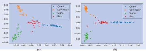
Figure 5. Exemplary centroid features of one ticker for 24 months. The solid lines indicate the actual values over the months, the dashed horizontal lines indicate the average over all months. (a) Number of orders (log scale) (b) Mean submission time (c) Cancellation rate.

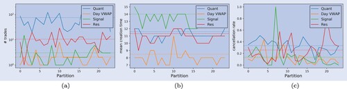
Table 5. Log-weighted average entropy and maximum affiliation probability of the agents.

Dimension	Entropy	Maximum Affiliation
Ticker	0.4	0.8
Time	0.5	0.76

Notes: The first row indicates both values for the consistency in ticker dimension. The second row indicates the values in time dimension.

Table 6. Affiliation of clusters to meta clusters for different tickers (time periods in parentheses).

	Meta Quant	Meta Day VWAP	Meta Signal	Meta Res
Quant	22 (23)	0 (0)	0 (0)	3 (1)
Day VWAP	0 (0)	25 (23)	0 (0)	0 (1)
Signal	0 (0)	0 (0)	24 (24)	1 (0)
Res	1 (0)	0 (0)	0 (0)	24 (24)

The average number of orders ( figure 5(a)) has shown to be one of the most relevant features in the clustering. Also the centroid values over time show strong discriminative behavior here. Quant is trading by far the most in all months, but one where Res trades similarly often. Day VWAP and Signal show a similar number of trades on the lowest level. This further supports our interpretation above and the embedding in figure 4 that Res lies in-between all clusters and sometimes much closer to Quant in terms of the number of trades.

The mean creation time depicted in figure 5(b) shows a both a discriminative and stable behavior, similar to the number of trades in figure 5(a). Quant and Res have a mean creation time around noon both types typically trade throughout the entire day. In contrast, Day VWAP trades very early in the morning and thus shows a mean submission time much earlier than the remaining agent types. For Signal, the mean submission time for different months fluctuates to a certain degree around the US market open. In general, the feature values from Day VWAP and Signal are well separated from Quant and Res.

For the cancellation rate, the situation differs. In general, the centroids' mean value fluctuates more and the time series of the values throughout different months are more overlapping. The dashed lines indicating the mean values of the different partitions still indicate the same ranking, where, in particular, Quant tends to have a higher cancellation rate indicating they more actively track the execution. Second highest is Res, which in several periods contains traders which tend to behave like Quant agents, potentially causing the increased cancellation rate. Day VWAP, apart from one large outlier, has the lowest cancellation rate of all clusters. In general, this feature illustrates that not all of the features used in the clustering process are stable or have the same ranking throughout different partitions.

The results of this section indicate high stability of the agent types presented in section 3.3. It consequently leads to assume that the observations are not random but rather follow a consistent pattern that exhibits different types of traders acting in the limit order market ecosystem. It is, however, not immediately clear whether the results are representative for other brokers. To ultimately verify this, a similar analysis of richer execution data sets consolidated from several brokers would be necessary, but highly unlikely to come by given the sensitivity of the data. Nonetheless, there are several reasons which make it rather unlikely that a similar analysis for another broker would lead to completely different results. Our data set does represent one of the largest market shares. This makes it likely that also a broad range of different traders interact with this broker. Furthermore, the stability analysis is done over two years of data and shows very consistent results. Making the assumption that traders change brokers from time to time and do not solely trade via a single broker leads to a varying set of clients. The temporal stability then implies that even though traders may trade more or less with a certain broker, the partition remains quite stable over time. Hence, one may assume that the overall picture in the market is rather similar. A difference may be caused by particular specialties of certain brokers. Consequently, we expect the agent types to be similar but potentially with different sizes, both in terms of agents but also in terms of traded volume.

4. Decomposition of order flow

This section reviews the properties of the order flow components which were segmented by clustering the agents in section 3. This shall answer the question whether the aggregated flows of each cluster show different also show different dynamics. This section builds a change of perspective as we do not look at different traders but aggregate over a particular cluster as one component. First, we look at the sizes and activities of the components' flow. Following this, child order properties, profitability and the correlation of inventory with the price moves are analyzed to outline notable differences between the components.

Figure 6(a) illustrates the distribution of the number of orders for each of the order flow components, throughout 25 different instruments of the STOXX 600 in two years. The distributions differ substantially. While Day VWAP and Signal show a similar distribution in terms of numbers of trades per month, Quant exhibits the largest numbers of orders. Res is once more located in-between the Quant and Day VWAP/Signal. This matches and further intensifies our previous interpretation that Res is some mixture of the first three agent types. Table 7 also indicates that the majority of the trades are done by Quant, and only a small fraction by Day VWAP and Signal.

Figure 6. Distribution of the number of trades and the executed quantity. (a) Number of submitted orders (b) Fraction of executed quantity.

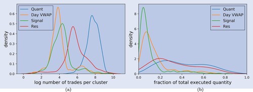
Table 7. Average values of the distributions of clients, trades and executed quantities across different clusters.

	Quant	Day VWAP	Signal	Res
Number of orders	0.69	0.06	0.06	0.20
Executed qty	0.41	0.15	0.11	0.34

The fraction of the total executed quantity from each of the single data slices is indicated in figure 6(b). The distributions of the fractions from Quant and Res show a similar shape. The same holds for Day VWAP and Signal. In fact, the sum of the executed quantity from Quant and Res does not vary much due to their strong negative correlation. The fraction of Res tends to increase when a trader from Res behaves rather like a Quant trader or potentially as a mixture of Quant, Day VWAP and Signal. In comparison to the very small number of orders submitted by Day VWAP and Signal, the actual executed quantity is much higher. In other words, while Day VWAP and Signal tend to account for only a small fraction of the number of orders, their contribution to the overall executed quantity is much larger since the orders are generally larger and/or lead to higher execution size (for example, due to fewer cancellations and longer execution). The mean fractions are displayed in the ‘Executed qty’ row of table 7.

4.1. Heterogeneity of child orders

This section reviews the differences of the four different components regarding the child orders which are sent to different venues. This may give further insights into the degree to which the order flow components differ not only at parent order, but also at the child order level. Table 8 shows a summary of the orders submitted to exchanges for one exemplary $B_{i,t}$. These sample results are for BATS.L for the month of December 2019. The numbers are normalized either by the mean of the corresponding statistic or by their sum.

Table 8. Aggregated statistics of child orders by clusters.

	C-Quant	C-Day VWAP	C-Signal	C-Res
# Child Orders	0.88	0.02	0.03	0.06
Mean Order Qty.	0.23	0.42	2.74	0.61
Median Order Qty.	0.29	0.28	3.11	0.33
Std Order Qty.	0.52	0.61	2.02	0.85
Mean Exec Qty.	0.12	0.18	3.53	0.17
Median Exec Qty.	0.70	0.75	1.76	0.79
Std Exec Qty.	0.33	0.40	2.95	0.31
DMA Ratio	2.27	0.03	1.63	0.07
Cancellation Ratio	1.07	0.90	1.09	0.94
Median Distance to Best Price	0.52	1.81	0.90	0.77

Notes: This table shows the total number of submitted child orders, the ratio of orders which were sent due to direct market access, the ratio of child orders which were cancelled, the mean, median and standard deviation for both order quantity and the executed quantity of orders. The last row shows the median distance of a limit order from the best opposite price. The number of child orders is normalized by the sum of all clusters; the remainder of the statistics are normalized by the mean of the four clusters.

In line with the observations regarding the number of orders and executed quantity from figure 6(a-b), the number of child orders submitted by Quant is by far the largest. Furthermore, the quantitative agents have the highest direct market access (DMA) ratio. This means these child orders come from parent orders that skip the processing of the broker's execution algorithms, hence primarily using the broker as a platform to send their orders to a venue. The DMA ratio is also high for the Signal component. In this particular segmentation, Signal contains one agent that heavily and exclusively trades with DMA orders leading to both an unusually high DMA and cancellation rate. This may be an agent which rather belongs to the Quant cluster and impacts the statistics of the Signal order flow component. For the Res and Day VWAP clusters, the DMA ratio is almost zero, and only around 75% of the child orders get cancelled.

Regarding the order and execution sizes of child orders, the orders of Quant have the lowest mean and standard deviation, as indicated in table 8. Signal has by far the highest mean order and execution quantity. A significantly higher mean compared to median indicates the presence of outliers for all clusters, which might be caused by larger orders placed in dark venues. In particular, component Signal exhibits many executions in dark venues for this month, as mentioned in section 3.3, hence rendering a large mean order quantity more plausible. As for the median, the execution quantities are significantly lower than the order sizes. One reason for this may be partially filled orders – in particular, in dark venues. Note that we exclude child orders without any partial fills for the present statistics.

Median Distance to Best Price indicates the relative price level at which the child orders of the particular component tend to be placed (i.e. this can be construed as a proxy for aggressiveness or urgency). Again, the median is displayed due to its robustness. Quant child orders are placed closest to the best price. The median distance from the best price for Res and Signal is roughly similar, while the orders from Day VWAP tend to be placed, when compared to child orders from the other clusters.

Lastly, we look at daily net inventory of the different components' child orders, the sum of the signed traded sizes (positive for buy, negative for sell) submitted by a cluster during one day. Table 9 indicates the mean cumulative inventory for one exemplary month. In particular, Quant appears to have been a net seller, while the remaining clusters were net buyers in that particular month during which the corresponding stock showed a positive return.

Table 9. Table indicating the mean cumulative inventory of the clusters.

	C-Quant	C-Day VWAP	C-Signal	C-Res
Average inventory	−0.62	0.12	0.11	0.16

Note: Values are normalized with the absolute inventory of the clusters.

Tables 10 and 11 indicates the correlation between the components over the whole duration and all instruments for both the net inventory as well as the order flow imbalance³. Clusters Signal and Res exhibit the strongest correlation. However, the correlations obtained are mostly statistically insignificant. Regressing the net inventory or the order flow imbalance of one cluster on any of the three other components, the coefficients rarely show any significant deviations from zero on instrument basis. For only very few instruments, weak significant correlations can be found, but the average p-value over all instruments considered here is around 0.25. We furthermore fit regressions over several instruments but a smaller time horizon, under the assumption that the correlations may change over time. Again, few variables show a persistent significance throughout time and the resulting $R^2$ are very low. This indicates that, despite significance for few variable combinations, the explanatory power is small.

Table 10. Correlation matrix of net inventory between different components.

	Quant	Day VWAP	Signal	Res
Quant	1.00	−0.05	−0.02	−0.04
Day VWAP	−0.05	1.00	0.00	−0.03
Signal	−0.02	0.00	1.00	−0.09
Res	−0.04	−0.03	−0.09	1.00

Table 11. Tables indicating the correlation of the order flow imbalance between different components.

	Quant	Day VWAP	Signal	Res
Quant	1.00	−0.07	0.00	−0.11
Day VWAP	−0.07	1.00	−0.02	−0.04
Signal	0.00	−0.02	1.00	−0.03
Res	−0.11	−0.04	−0.03	1.00

The resulting both inconclusive as well as insignificant correlation between the net inventories (OFIs respectively) indicates that not only the behavior between the cluster differs quite substantially but they are also independent from each other in the way they accumulate inventory. One possible reason for this may be that different trader types trade different strategies which are either not correlated at all (leading to insignificant correlations). Another explanation would be that changes depend on the market environment as some strategies may only correlate during certain market conditions. In particular, the first makes sense since the trading types seem to act on different time scales in the market. The most persistent observation is a slight negative correlation between Quant and the remainder of the order flow components which, however, is relatively weak.

4.2. Profitability

In section 3, we showed that traders using execution services may be summarised into different clusters. These trader types have different properties when it comes to the type of orders they send. This leads to the assumption that the objectives of the segmented agent types may differ as well, for example, with respect to their horizon of investment. To this end, we analyze the hypothetical profit and loss (PnL) for each order flow component, in order to investigate structural differences in the returns of the components' trades. We remark that this PnL is hypothetical as it does not refer to the actual inventory of the trader. For example, it may be that a trader is not holding a position for the respective future horizon of time, or that it is actually unwinding a short position instead of building a long position, or the holding period is different. It much rather represents the average PnL of the respective component, at a certain fixed time horizon.

To investigate the hypothetical profitability of each component, we compute the PnL of each trade via (16) $Pn{L}_t^l=-\mathrm{s}\mathrm{i}\mathrm{g}\mathrm{n}\left(q^{target}\right)\log \left(\frac{p_{t+l}}{p^{exec}}\right),$(16) where $p^{exec}$ is the volume-weighted execution price of the corresponding parent order. $q^{target}$ is the target quantity of the parent order, as specified in Definition 2.3, and $-\mathrm{s}\mathrm{i}\mathrm{g}\mathrm{n}\left(q^{target}\right)$ the negative sign of the return. If, for example, $q^{target}>0$ the order is a sell order, thus we multiply the log-return with $-1$. For some time step t + l, $p_{t+l}$ denotes the closing price at t + l, where we consider trading days as increments. For l = 0, $p_t$ corresponds to the close price of the day when the corresponding trade happens.

The volume weighted average price of a parent order's execution $p^{exec}$ is computed via (17) $p^{exec}=\frac{1}{q^{exec}}\sum _{x\in {\mathcal{X}}^{exec}}{q}_x\cdot p_x,$(17) where $q_x$ and $p_x$ indicate the quantity and the price of each execution in ${\mathcal{X}}^{exec}$ of the corresponding parent order. Finally, we compute the expected PnL for each component $k\in \{1,\dots ,K\}$ of trades at day t, as $\mathbb{E}\left(Pn{L}_{t,k}^l\right)$ by averaging over all returns for a given l, t, k. The result is a daily time series for different lags $l\in \{0,1,10,20\}$ and different components $k\in \{1,\dots ,K\}$, where each element is the average PnL of the trades that occurred on that particular day. The same computation is done using market excess return, where we subtract the future market return from the instrument's future return, for the PnL computation in equation (16(16) $Pn{L}_t^l=-\mathrm{s}\mathrm{i}\mathrm{g}\mathrm{n}\left(q^{target}\right)\log \left(\frac{p_{t+l}}{p^{exec}}\right),$(16) ).

Table 12 indicates the average expected PnL in basis points for 2018 and 2019 for 25 instruments. From trade to close, Quant appears to be the only order flow component generating a slight profit over the period covered here. This indicates that Quant is potentially pursuing more intraday/short-term strategies. This is supported by the statistical significance of the market excess return of Quant for l = 1. For Signal, the 20-day return (both raw return and market excess return) is the largest and furthermore significantly different from 0 to a confidence level of $95\mathrm{\%}$. Even though this is not a realized return, it gives reason to assume this agent type has some medium-frequency edge it is trading. Furthermore, Signal showing the smallest PnL on the same trading day (l = 0) supports our interpretation of Signal given in section 3 that this component is not aiming for a profit that realizes within the same day. It may well be that the Signal agent type trades mean reversion patterns which realize only after around a month. Apart from that, Day VWAP shows a slight outperformance on the l = 1 horizon.

Table 12. Table indicating the average $\mathbb{E}\left(Pn{L}_k^l\right)$ for agent types in basis points (bps).

	Gross return				Excess
	l = 0	l = 1	l = 10	l = 20	l = 1, excess	l = 10, excess	l = 20, excess
Quant	0.38	0.72	3.39	3.76	0.78${}^{\ast }$	3.78	2.83
Day VWAP	−0.25	1.54	−2.04	−3.95	1.42	0.15	1.44
Signal	−0.47${}^{\ast }$	−0.43	3.09	13.17${}^{\ast }$	0.32	2.65	10.63${}^{\ast }$
Res	0.08	0.37	−1.36	−1.51	0.52	−2.24	−2.19

Notes: The suffix _excess indicates market excess returns over the STOXX 600 baseline. A * behind the return in basis points indicates significance using a one-sample t-test and with a confidence level of $95\mathrm{\%}$.

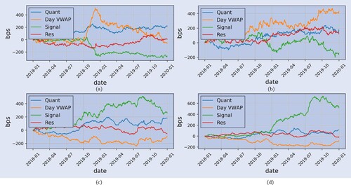
Additionally, figure 7 shows the cumulative hypothetical PnL for each component. In line with the observations from table 12, Signal is clearly outperforming the other agent types on a 20-day horizon (lower right plot) while having the worst performance from trade to close and to t + 1 (upper plots). Nonetheless, all Sharpe ratios (risk-adjusted returns) are very close to zero.

Figure 7. Cumulative PnL $\mathbb{E}\left(Pn{L}_{t,k}^l\right)$ in basis points (bps) of agent types over different time horizons, $l=\{0,1,10,20\}$. (a) l = 0 (b) l = 1 (c) l = 10 (d) l = 20.

4.3. Order flow imbalances during volatile periods

While some components show differences in their expected returns with respect to the trading horizon, it stands to question to which degree the components' order flow on a particular day is correlated with the return of the day. In particular, how does the order flow of different agent types behaves when markets move substantially. To this end, we compute the order flow imbalance (OFI) for each instrument via the following measures (18) $OF{I}^{C_k}=\frac{\sum _{p\in {\mathcal{X}}^k}{q}^{exec}}{\sum _{p\in {\mathcal{X}}^k}\left|q^{exec}\right|},$(18) and (19) $OF{I}^{ADV}=\frac{\sum _{p\in {\mathcal{X}}^k}{q}^{exec}}{\mathrm{A}\mathrm{D}\mathrm{V}},$(19) where ${\mathcal{X}}^k$ is the set of parent orders from cluster k on a given day. We compute the imbalance of the order flow in two ways. The first imbalance is shown in equation (18(18) $OF{I}^{C_k}=\frac{\sum _{p\in {\mathcal{X}}^k}{q}^{exec}}{\sum _{p\in {\mathcal{X}}^k}\left|q^{exec}\right|},$(18) ) is normalized by the total executed quantity of the cluster, hence called $OF{I}^{C_k}$. The second imbalance is shown in equation (19(19) $OF{I}^{ADV}=\frac{\sum _{p\in {\mathcal{X}}^k}{q}^{exec}}{\mathrm{A}\mathrm{D}\mathrm{V}},$(19) ) is normalized by the average daily volume (ADV) from the last 20 days and denoted as $OF{I}^{ADV}$. This is to take into account that a large OFI, as defined in equation (18(18) $OF{I}^{C_k}=\frac{\sum _{p\in {\mathcal{X}}^k}{q}^{exec}}{\sum _{p\in {\mathcal{X}}^k}\left|q^{exec}\right|},$(18) ), does not necessarily mean a large impact to the market during the particular day. That is because the total traded volume of the cluster might only be a small fraction of the daily volume. In contrast, equation (19(19) $OF{I}^{ADV}=\frac{\sum _{p\in {\mathcal{X}}^k}{q}^{exec}}{\mathrm{A}\mathrm{D}\mathrm{V}},$(19) ) makes different values of the same day more comparable across different clusters, and is large only if a component's net inventory is large in relation to the historical ADV. E.g. one cluster might have a large OFI in terms of own orders but still a very small OFI measured on the ADV due to small traded volume.

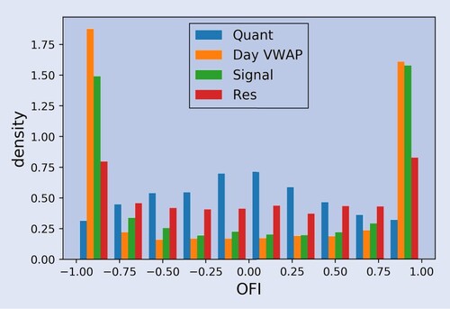
Figure 8 shows a histogram of the OFI as in equation (18(18) $OF{I}^{C_k}=\frac{\sum _{p\in {\mathcal{X}}^k}{q}^{exec}}{\sum _{p\in {\mathcal{X}}^k}\left|q^{exec}\right|},$(18) ) to simplify comparison. Quant stands in contrast to the other three components. The net order flow peaks around zero, while the other order flow components have two peaks at zero and one. In particular, the aggregated order flow from Quant tends to be rather neutral in terms of order flow imbalance, which can be due to two reasons. First, Quant trades much more often (albeit smaller sizes) and thus facilitates order flow imbalances closer to zero. Second, Quant pursues more intraday/medium frequency strategies without accumulating larger positions.

Figure 8. Order flow imbalance by cluster, during days of returns with large magnitude.

The correlation of the OFI with the log return from open to close (logOC) is shown in table 13 (via equation (18(18) $OF{I}^{C_k}=\frac{\sum _{p\in {\mathcal{X}}^k}{q}^{exec}}{\sum _{p\in {\mathcal{X}}^k}\left|q^{exec}\right|},$(18) )) and in table 14 (via equation (19(19) $OF{I}^{ADV}=\frac{\sum _{p\in {\mathcal{X}}^k}{q}^{exec}}{\mathrm{A}\mathrm{D}\mathrm{V}},$(19) )). Day VWAP and Res show the clearest picture. For both the case of days of large returns of the particular instrument (left columns), as well as days of large returns of the index (right columns), Day VWAP and Res exhibit a fairly strong positive correlation. This holds for the net inventory scaled by the traded volume of the particular component ( table 13), as well as the net inventory scaled by the market volume ( table 14). In fact, the correlation of $OF{I}^{ADV}$ with both the instrument and the index return are larger than the correlation of $OF{I}^{C_k}$ with the return. In other words, when these clusters accumulate net inventory which is also large in terms of the average daily volume, the instrument is likely to also exhibit a larger return. A possible reason for this may be that the order flow becomes a driving factor in the market.

Table 13. Correlation between OFI and returns of stocks (column logOC) and return of the index (column logOC_index).

Cluster	logOC	logOC_index
Quant	−0.0301	0.0113
Day VWAP	0.1590	0.0229
Signal	−0.1506	0.0499
Res	0.1102	0.1616

Note: $OF{I}^{C_k}$ as in equation (18(18) $OF{I}^{C_k}=\frac{\sum _{p\in {\mathcal{X}}^k}{q}^{exec}}{\sum _{p\in {\mathcal{X}}^k}\left|q^{exec}\right|},$(18) ).

Table 14. Correlation between OFI and returns of stocks (column logOC) and return of the index (column logOC_index).

Cluster	logOC	logOC_index
Quant	0.1368	0.0833
Day VWAP	0.2044	0.1416
Signal	−0.0441	−0.0794
Res	0.2189	0.2390

Note: $OF{I}^{ADV}$ as in equation (19(19) $OF{I}^{ADV}=\frac{\sum _{p\in {\mathcal{X}}^k}{q}^{exec}}{\mathrm{A}\mathrm{D}\mathrm{V}},$(19) ).

Signal is the only cluster exhibiting a fairly large negative correlation with negative returns of the instruments. This correlation seems to be less strong when the net inventory is large as defined in equation (19(19) $OF{I}^{ADV}=\frac{\sum _{p\in {\mathcal{X}}^k}{q}^{exec}}{\mathrm{A}\mathrm{D}\mathrm{V}},$(19) ). A reason for this may be that due to the high participation rate, Signal becomes a driving factor of the market, similar to Day VWAP and Res above. The correlation with the index is less clear and varies between $OF{I}^{C_k}$ and $OF{I}^{ADV}$. However, it seems that the index is more likely to decrease if the net inventory is large, also based on the average daily volume of the corresponding stock.

Quant shows the lowest correlation of net inventory scaled with total trade size, with both the daily return as well as the index (−0.03 and 0.01, respectively). This is to be expected, taking into account figure 8 which shows the tendency of Quant to keep a net inventory closer to zero. For net inventories which are large measured on the total market volume following equation (19(19) $OF{I}^{ADV}=\frac{\sum _{p\in {\mathcal{X}}^k}{q}^{exec}}{\mathrm{A}\mathrm{D}\mathrm{V}},$(19) ), however, the correlation also seems to turn stronger. Similar as for Day VWAP and Res, if the net inventory is large measured on the ADV, the cluster becomes more of a market driver and a higher correlation with the daily return can be observed.

5. Towards a heterogeneous parent order model

As illustrated in the order process in figure 1, limit orders sent through execution services are usually part of a larger parent order. This section outlines how to capture the most important heterogeneous properties for each of the components extracted in section 3. Heterogeneous parent order flow can then be modeled. The resulting flow can then be processed, resulting in child orders into the LOB as depicted in figure 1 via known execution and order routing algorithms, some of which are well studied in the literature. Modeling the flow of these components itself without the direct scheduling and execution can additionally be of high interest to brokers, as this can possibly improve the broker's knowledge and service to clients. Rather than aiming to replicate and fit the data to the full extent, this section's remainder is designed as a starting point for future research. It also further underpins the structural differences between the different clusters, which have been outlined in the previous sections. Furthermore, we assume independence between the flows presented in the following, due to the absence of a significant correlation structure between the components.

5.1. Quant

As outlined in section 3, the Quant order flow component is submitting orders throughout the day. Figure 9(c) suggests the U-shaped intraday pattern commonly observed in trading behavior of limit order books (Cont 2011). In the morning and towards closing time of the market, the intensity of the orders increases. Quant order sizes are of mostly small size and typically executed in just a few child orders. This, however, does not imply that only one order is sent to the exchange.

Figure 9. Aggregated parent order flow distributions for one stock, over two years, for Quant. (a) Order counts: QUANT order flow. (b) Order size distribution: QUANT order flow (c) Submission times (d) Fraction of buy orders.

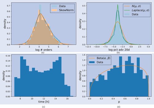
As per modeling the Quant order flow component, we suggest a non-homogeneous Poisson process. Orders arrive proportional to the intraday shape shown in figure 9(c). The expected total number of orders can be easily fitted with a skewed normal distribution as shown in figure 9(a). Every order then comes with a size q which can be drawn from a Laplacian distribution as indicated in figure 9(b). What is missing for the specification of the parent order is the side. As noted, the ratio in which Quant buys or sells is not constant. Hence, a possibility is to model the buy ratio of the Quant component with a Beta distribution. The fit for an exemplary ticker is indicated in figure 9(d).

The plots in figure 9 show that all necessary quantities of the Quant parent orders can be well fit with simple distributions. Once these parent orders are modeled, it can be simulated how these flow to different venues. The execution of the Quant orders could be done with the Almgren-Chriss optimal execution framework, first presented in Almgren and Chriss (2001). The execution generally consists of only very few, if not just one child order, and the execution time is very short.

5.2. Day VWAP

As outlined in table 3, Day VWAP mainly sends parent orders in the early morning around the market opening. The total number of parent orders is quite small, while execution generally takes place throughout the entire day. A model for these orders is thus quite simple and can be done without any time dependence, since it can be assumed all orders are submitted at market open (i.e. t = 0). The orders are then executed throughout the day proportional to some estimated volume profile.

Consequently, it suffices to know how the sum of all buy (respectively, sell) orders is distributed, which is then executed as one large buy order (respectively, sell order). Denoting ${\mathcal{X}}^{DayVWAP}$ as the set of all parent orders from the Day VWAP component for a given day, the quantities of interest are $\sum _{p\in {\mathcal{X}}^{DayVWAP}}\left(q^{target}{)}_{-}\mathrm{a}\mathrm{n}\mathrm{d}\sum _{p\in {\mathcal{X}}^{DayVWAP}}\right(q^{target}{)}_{+},$ where the first term builds the cumulative size of all Day VWAP buy orders, and the second term all Day VWAP sell orders. The Day VWAP component then consists of two (aggregated) parent orders with t = 0 as submission time and the corresponding target quantities. In figure 10, it can be seen that the cumulative buy/sell sizes of the orders are fairly well fit by a skewed normal distribution.

Figure 10. Aggregated parent order sizes (on a log scale) for one stock over two years for Day VWAP.

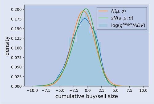
The aggregated buy and sell Day VWAP orders are executed following to the volume profile of the previous day or some other modeled volume profile.

5.3. Signal

The Signal cluster as outlined in table 3 sends quite large orders and executes them in a relatively short horizon. This lets assume Signal is a more aggressive player in the LOB, moving the LOB in a certain time horizon.

As per modeling the Signal component, we suggest a non-homogeneous Poisson process similar to Quant. The intraday shape shows a completely different pattern, as illustrated in figure 11(c). The distribution of total number of orders is shown in figure 11(a) and can be easily fit with a Geometric distribution. The quantities of each parent order fit a skewed normal distribution as indicated in 11(b), for the same exemplary ticker as for above.

Figure 11. Aggregated parent order flow distributions for one stock over two years for Signal. (a) Order counts (b) Order sizes (c) Submission times.

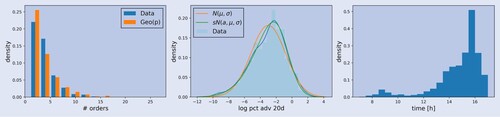
A large proportion of the Signal component consists of closing session-related orders. These are removed since they do not form part of the continuous trading session, and only pertain to the end-of-day closing session. Once the parent orders are modeled, they can be fed into the execution pipeline which can be further modeled with known approaches. We suggest the execution of the Signal orders is performed similarly to the Quant orders using the Almgren-Chriss framework Almgren and Chriss (2001). The detailed execution, however, is well outside of the scope of this work and not pursued here. Note that orders from Signal are substantially larger than those from Quant, which – together with the frequency of orders and the intraday pattern – constitutes the main difference between the two clusters.

5.4. Res

Both the representative features in table 3 as well as the embedding of the first stage clustering in figure 4 indicate that Res lies in between the remainder of the other clusters. In addition, the confusion matrices in table 6 confirm that whenever there exists instability in the market segmentation, one of the remaining clusters is indistinguishable from Res.

One simple approach to model the Res is as a random mixture of C-Quant, C-Day VWAP and Res. This can be done for instance via a Dirichlet distribution whose parameters entail the expected weights between the three other clusters. The order volume of Res can then simply be allocated to the corresponding components.

6. Conclusion

Electronic markets involve a variety of market participants with different frequencies, trading horizons and information sets, leading to a heterogeneous order flow with distinct components corresponding to different types of agents and strategies. We have introduced in section 2, a new representation of the limit order book which accounts for this heterogeneity by keeping track of the origin of each order by agent type. This representation, which corresponds to a level of information intermediate between an anonymized view and a fully omniscient view, is a realistic representation of the information available to a broker.

To investigate the heterogeneity of those agents which make use of brokers, trade execution data was analyzed. Results show these agents may be summarised in four representative clusters, which differ substantially in both their trading behavior as well as the order flow induced in the limit order book by the parent orders. In particular, trading frequency, trade size but also order submission time and execution strategies show notable differences between these agent types which gives evidence that some heterogeneity may be assumed. The insights were used to propose a simple model for parent order flow of each cluster in order to capture some of the heterogeneous dynamics of the different trader types in section 5.

Our results complement those of Kirilenko et al. (2017). We do recover the ‘fundamental buyers/sellers’ and ‘opportunistic traders’ classes from Kirilenko et al. (2017), but Kirilenko et al. (2017) mainly focus on HFTs and market makers which are excluded from our data as they have their own execution platforms. On the other hand, in contrast to Kirilenko et al. (2017), we are able to access parent orders across several tickers, which gives us more information on agents trading styles. This enables to show that the agent types presented in section 3.3 are stable over longer time periods and across different stocks.

The results of this study and Kirilenko et al. (2017) provide evidence for the strong heterogeneity of order flow in limit order markets and suggest that a realistic model for this order flow should account for its multiple components operating at different frequencies.

Disclosure statement

No potential conflict of interest was reported by the author(s).

Additional information

Funding

Felix Prenzel has been supported by the EPSRC Centre for Doctoral Training in Mathematics of Random Systems: Analysis, Modelling and Simulation (EP/S023925/1).

Notes

1 https://www.lobsterdata.com/

2 See Hastie et al. (2009) for the detailed algorithm.

3 The order flow imbalance is computed with the net inventory divided by the total trade volume of the component. A more detailed explanation can be found in section 4.3.

Appendices

Appendix 1. Feature table

Table A1. Feature list used for the clustering.

Feature name	Explanation
Buy ratio	Pct. of client orders which is a buy order
Cancellation ratio	Pct. of client orders which are cancelled before full execution
# Trades per month	Number of trades per month.
Inventory	Mean inventory accumulation of a client on a given day
NO Limit price ratio	Percentage of the client's orders for which no limit price has been specified (maximum/minimum price for execution of child orders)
Maximum order creation time	Latest time at which a client submits an order
Mean order creation time	Average time at which a client submits an order
Mean order size (ratio of ADV)	Mean order size measured on the average daily volume of the last 20 days, execution may be less.
Mean momentum (bps)	Mean momentum of entire trading day measured in basis points (bps)
Mean percentage of volume	Mean percentage of traded volume during trade horizon (visible fills + dark fills) / (visible market volume), exceeding 100 is indicator for larger placements in dark venues
Mean volatility	Mean volatility during which a client trades measured on the last 20 days
Minimum order creation time	Earliest time a client creates an order
# Active days per month	Number of days a client trades per month
Mean # orders per active day	Number of orders a client trades if it trades during a day
Standard deviation # orders per active day	Standard deviation of the number of orders of days during which a client places at least one order
Standard deviation of order creation time	Standard deviation of a client's creation time
Standard deviation order size	Standard deviation of a clients order size
Total order size	Cumulative trade size measured on the average daily volume of the last 20 days. Indication of how much a client in average trades at all

Notes: All features are computed on the base of a one-month dataset. For instance, #Trades indicates the number of trades for a particular client per month. The creation time, measured from the time passed since midnight is set to a minimum of 7 as some clients, sending their orders on the evening before disrupt the feature distribution. 7 am in this case involves all orders sent before market opening.

Appendix 2. Disclaimer

Opinions and estimates constitute our judgement as of the date of this Material, are for informational purposes only and are subject to change without notice. This Material is not the product of J.P. Morgan's Research Department and therefore, has not been prepared in accordance with legal requirements to promote the independence of research, including but not limited to, the prohibition on the dealing ahead of the dissemination of investment research. This Material is not intended as research, a recommendation, advice, offer or solicitation for the purchase or sale of any financial product or service, or to be used in any way for evaluating the merits of participating in any transaction. It is not a research report and is not intended as such. Past performance is not indicative of future results. Please consult your own advisors regarding legal, tax, accounting or any other aspects including suitability implications for your particular circumstances. J.P. Morgan disclaims any responsibility or liability whatsoever for the quality, accuracy or completeness of the information herein, and for any reliance on, or use of this material in any way.

References

- Almgren, R. and Chriss, N., Optimal execution of portfolio transactions. J. Risk, 2001, 3, 5–40.
- Barbon, A., Di Maggio, M., Franzoni, F. and Landier, A., Brokers and order flow leakage: Evidence from fire sales. J. Finance, 2019, 74, 2707–2749.
- Belkin, M. and Niyogi, P., Laplacian eigenmaps and spectral techniques for embedding and clustering. In Proceedings of the Advances in Neural Information Processing Systems, pp. 585–591, 2002.
- Bouchaud, J.P., Mézard, M. and Potters, M., Statistical properties of stock order books: Empirical results and models. Quant. Finance, 2002, 2, 251–256.
- Brogaard, J., Hendershott, T. and Riordan, R., High-frequency trading and price discovery. Rev. Financ. Stud., 2014, 27, 2267–2306.
- Brogaard, J., High frequency trading and its impact on market quality. Working Paper, Northwestern University Kellogg School of Management, No. 66, 2010.
- Byrd, D., Hybinette, M. and Balch, T.H., Abides: Towards high-fidelity market simulation for ai research. arXiv preprint arXiv:1904.12066, 2019.
- Cont, R., Statistical modeling of high-frequency financial data. IEEE. Signal. Process. Mag., 2011, 28, 16–25.
- Cont, R. and De Larrard, A., Price dynamics in a Markovian limit order market. SIAM J. Financial Math., 2013, 4, 1–25.
- Cont, R., Stoikov, S. and Talreja, R., A stochastic model for order book dynamics. Oper. Res., 2010, 58, 549–563.
- Di Maggio, M., Franzoni, F., Kermani, A. and Sommavilla, C., The relevance of broker networks for information diffusion in the stock market. J. Financ. Econ., 2019, 134, 419–446.
- Gould, M.D., Porter, M.A., Williams, S., McDonald, M., Fenn, D.J. and Howison, S.D., Limit order books. Quant. Finance, 2013, 13, 1709–1742.
- Hagströmer, B. and Nordén, L., The diversity of high-frequency traders. J. Financ. Mark., 2013, 16, 741–770.
- Hasbrouck, J. and Saar, G., Low-latency trading. J. Financ. Mark., 2013, 16, 646–679.
- Hastie, T., Tibshirani, R. and Friedman, J., The Elements of Statistical Learning: Data Mining, Inference, and Prediction, 2009 (Springer: New York).
- Hendershott, T., Li, D., Livdan, D. and Schürhoff, N., Relationship trading in over-the-counter markets. J. Finance, 2020, 75,683–734.
- Kirilenko, A., Kyle, A.S., Samadi, M. and Tuzun, T., The flash crash: High-frequency trading in an electronic market. J. Finance, 2017, 72, 967–998.
- MacQueen, J., Some methods for classification and analysis of multivariate observations. In Proceedings of the fifth Berkeley Symposium on Mathematical Statistics and Probability, Vol. 1, pp. 281–297, 1967 (Oakland).
- Meila, M. and Shi, J., A random walks view of spectral segmentation. In Proceedings of the Eighth International Workshop on Artificial Intelligence and Statistics, pp. 203–208, 2001 (PMLR).
- Moallemi, C.C. and Yuan, K., A model for queue position valuation in a limit order book. Columbia Business School Research Paper No. 17-70, 2016.
- Ng, A.Y., Jordan, M.I. and Weiss, Y., On spectral clustering: Analysis and an algorithm. In Proceedings of the Advances in Neural Information Processing Systems, pp. 849–856, 2002 (MIT Press: Boston).
- Shi, J. and Malik, J., Normalized cuts and image segmentation. IEEE. Trans. Pattern. Anal. Mach. Intell., 2000, 22, 888–905.
- Sirignano, J. and Cont, R., Universal features of price formation in financial markets: Perspectives from deep learning. Quant. Finance, 2019, 19, 1449–1459.
- Smith, E., Farmer, J.D., Gillemot, L.s. and Krishnamurthy, S., Statistical theory of the continuous double auction. Quant. Finance, 2003, 3, 481–514.
- Van Kervel, V. and Menkveld, A.J., High-frequency trading around large institutional orders. J. Finance, 2019, 74, 1091–1137.
- Von Luxburg, U., A tutorial on spectral clustering. Stat. Comput., 2007, 17, 395–416.
- Vyetrenko, S., Byrd, D., Petosa, N., Mahfouz, M., Dervovic, D., Veloso, M. and Balch, T.H., Get real: Realism metrics for robust limit order book market simulations. arXiv preprint arXiv:1912.04941, 2019.
- Zhang, Z., Zohren, S. and Roberts, S., Deeplob: Deep convolutional neural networks for limit order books. IEEE. Trans. Signal. Process., 2019, 67, 3001–3012.