


 ?Mathematical formulae have been encoded as MathML and are displayed in this HTML version using MathJax in order to improve their display. Uncheck the box to turn MathJax off. This feature requires Javascript. Click on a formula to zoom.
Abstract
Leveraged and inverse exchange-traded funds seek daily returns equal to fixed multiples of indexes' returns, but the ensuing rebalancing costs create a tension between a high correlation with the index and a low average deviation from the leveraged index' performance. With proportional trading costs, we find that the optimal replication policy is robust to the index' dynamics and obtain a sufficient statistic for index replication performance, the implied spread, which is insensitive to risk-premia and enables comparisons of funds tracking different factors of an index. Overall, the impact of trading costs on replication performance is comparable to or higher than the effect of management fees.
1. Introduction
Leveraged and inverse exchange-traded funds (LIETFs) aim to deliver daily returns that scale an index' return by a constant factor. Introduced in the United States in 2006, the 12 funds available at the end of that year barely held $2 billion. Since then, new funds have become available for equity indexes specific to countries and industry sectors, bonds, commodities, currencies, and real estate. At the end of 2022, over 240 leveraged or inverse funds held over $65 billion in assets, almost all of them managed by two firms, Profunds and Direxion.Footnote1
Typical factors for these funds range from for inverse funds to
for leveraged ones, which may lead to large losses in turbulent markets, thereby raising regulators' concerns—and doubts. In 2015, an SEC proposal sought to cap leverage to 150%, but was not implemented. In 2017, the SEC initially approved the listing of funds with factors of
, only to later reconsider its decision.Footnote2 Overall, LIETFs appear to have grown faster than their research.
Despite the ostensible simplicity of LIETFs, even the determinants of their returns are not fully understood. For example, since inception in 2006 to the end of 2022, the ProShares Ultra S&P500 (SSO), which doubles the daily return of the S&P 500 index, had a cumulative return of 396%. However, compounding the daily returns of its benchmark strategy would imply a gross (i.e. before management fees) theoretical return of 594%. Net of such fees, the return would have been 486%, which still leaves an unexplained gap of 1.01% per year.
Such deviations of LIETF returns from their benchmarks are economically significant, and of the same order of magnitude as management fees. They are also systematic, and call for sharper analytical tools to understand and evaluate the performance of these funds, which this paper aims to provide.
LIETFs represent shares of ownership of an asset pool, managed so that its exposure to the underlying index matches approximately the target factor of the fund. In practice, for leveraged funds on indexes with liquid constituents such as the S&P 500, a fraction of the exposure is achieved by investing in the index' components. The remainder of the exposure—for inverse funds, all of the exposure—is obtained through over-the-counter index swap contracts collateralized by the fund's assets, the bulk of which is in cash instruments. The funds' holdings and net asset value are published daily.
The mechanism that keeps the shares of such funds aligned with their net asset value is the activity of authorized participants (typically market makers and broker dealers), who exchange blocks of funds' shares (creation units) for the underlying basket of securities at their net asset value (minus a transaction fee of approximately 0.10%). As a result, authorized participants quickly exploit arbitrage opportunities created by minimal departures of the market price of the fund's shares from its net asset value, thereby ensuring that the former closely tracks the latter.
Keeping a constant leverage ratio requires rebalancing the portfolio daily, as to keep the amount of index exposure near the target multiple of the fund's value: both leveraged and inverse funds buy the index when it increases and sell it when it decreases (Cheng and Madhavan Citation2009). Rebalancing requires a significant amount of trading: for example, a typical 1% daily return (one standard deviation, for an annual volatility of 16%) implies a daily turnover of 2% for a fund with factor or
, 6% with factors
or
, and a remarkable 12% with factor
.Footnote3 Such trading volume generates substantial trading costs, especially for funds with high leverage ratios and for indexes with high volatility and low liquidity. While funds managers seek to mitigate trading frictions using swaps and derivatives, the question is to what extent the trading costs generated by frequent rebalancing are responsible for the observed underperformance of LIETFs.
The tradeoff between correlation and underperformance underlies the two main metrics used to evaluate passive investment funds, which focus on the difference between the index' multiple and the fund's daily returns. The tracking error (), the annualized standard deviation of such difference, reflects the precision with which the fund mimics its target at a daily frequency. The tracking difference (
), the annualized average of such difference, measures the systematic gap between the benchmark index and the fund. Tracking error and tracking difference are the main indicators used by academics (Charteris and McCullough Citation2020), practitioners (Frino and Gallagher Citation2001, Johnson et al. Citation2013), and regulators (ESMA Citation2014) to evaluate the performance of ETFs.Footnote4
This tension raises two central problems for managers and investors. Fund managers need to trade as efficiently as possible to achieve the desired tracking error while minimizing the deviation from the leveraged index. Investors compare competing funds that differ in leverage ratios, tracking error, and tracking difference, and need performance measures that control for such differences. The contribution of this paper is to answer these questions in a model with arbitrary volatility dynamics, continuous trading, and trading costs proportional to volume, leading to two main results for managers and investors.
A manager's optimal replication policy is independent of volatility, while it depends only on the trading cost ε, the target factor Λ, and the desired tradeoff between tracking error and tracking difference, summarized by a positive parameter γ, which captures investors' aversion to tracking error. The manager should keep the fund's index exposure, as a multiple of the fund's assets, within the approximate thresholds
by minimally increasing and decreasing the fund's exposure as it reaches the lower and upper levels, respectively. In this formula, higher values of the parameter γ lead to a narrower no-trade region, which results in lower tracking error, higher trading costs, and consequently a more negative tracking difference. The formula is similar to the optimal trading boundaries arising in problems of optimal portfolio choice with transaction costs, with one crucial difference: here the approximate policy is insensitive to the index price dynamics, both volatility and expected return.Footnote5 Even as these boundaries remain constant, in more volatile times rebalancing is higher as the index position is more volatile, and boundaries reached more frequently.
The robust replication of leveraged funds has some analogies with the robust hedging of variance swaps, developed by Dupire (Citation1993), Neuberger (Citation1994), and Carr and Madan (Citation2001): if the underlying index follows a continuous process, the optimal replication policy does not depend on the particular volatility dynamics, and in the absence of frictions the replication is perfect. In the present context, such robustness remains valid in the presence of trading frictions, though the optimal strategy's performance does depend on realized volatility.
The optimal replication policy under frictions explains the underexposure puzzle observed by Tang and Xu (Citation2013), who report that average exposures of both leveraged and inverse funds in US markets are significantly smaller than their target factor. We confirm this effect in recent data on US funds and show that it is consistent with the model's predictions: though the optimal rebalancing boundaries are symmetric (at the first order) around the target factor, the fund's volatility is lower when its exposure is closer to zero, which increases the time spent at such smaller exposures and generates a bias towards zero for the average exposure. The effect is stronger for larger factors and more volatile indexes.
The main implication for investors is that a summary of a fund's overall tracking performance is the implied spread, defined as
(1)
(1)
This quantity estimates the hypothetical bid-ask spread that would make the investor indifferent between using the fund or replicating the index by trading with such a spread.
Formula (Equation1(1)
(1) ) offers a tool for comparing the performance of funds with different factors and tracking errors: the implied spread combines the tracking difference (
) and tracking error (
) in a single number, measuring the fund's performance after controlling for the factor Λ and the index' average volatility
, which otherwise magnify the effect of trading frictions. The formula implies that, holding the factor constant, an optimally managed fund that seeks to halve its (negative) tracking difference should be prepared to approximately double its tracking error. In addition, the formula does not depend on the index' risk premium, which is notoriously hard to estimate with precision.
Most implied spreads in US funds range between 2 and 20 basis points, with smaller spreads for funds with larger factors, implying that more volatile funds offer a better tradeoff between tracking difference and tracking error. An explanation for this phenomenon lies in the management fees charged by leveraged funds, which are nearly the same for funds with different factors, making funds with larger factors comparatively cheaper in their unit cost of exposure.
These findings shed new light on the growing literature on leveraged funds. Tang and Xu (Citation2013) report that leveraged funds deviate significantly from their benchmarks even after management fees, and separate tracking error into a compounding component, due to the convexity of leveraged returns, and a rebalancing component, due to trading frictionsFootnote6 . Wagalath (Citation2014) derives an asymptotic expression for the slippage that results from rebalancing at fixed intervals. Anderson et al. (Citation2012) note the sensitivity to trading frictions of risk-parity strategies, a popular class of leveraged strategies, and Anderson et al. (Citation2014) propose a leveraged performance attribution formula that emphasizes, in addition to transaction costs, the comovement between portfolio exposure and index return. The recent work of Dai et al. (Citation2022) studies the problem of continuous intraday replication of leveraged ETFs with quadratic transaction costs.
The paper is organized as follows: section 2 introduces the model and the optimization problem. Section 3 contains the main results on optimal leverage replication and performance evaluation ( theorem 3.1). Section 4 describes how the replication of LIETFs takes place in practice, providing a quantitative analysis of the trading costs associated to rebalancing. With such context, section 5 investigates the paper's implications empirically, focusing on families of leveraged and inverse ETFs traded in US markets. Section 6 discusses the robustness of the paper's results to risk-premia proportional to return variance, finite horizons, and discrete trading. Section 7 concludes. All proofs are in the appendix.
2. Model
The market has a safe asset earning an interest rate and a risky asset (the index) with ask (buying) price
, where
and with the index' bid (selling) price
, which implies a constant relative bid-ask spread of
, or, equivalently, constant proportional transaction costs. Here
is a standard Brownian motion on a filtered probability space
, while
is an adapted process such that
a.s. Volatility is integrable and stationary:
Assumption 2.1
The process satisfies
and is weakly ergodic with stationary variance
, i.e.
Thus the dynamics of the safe rate and volatility are essentially arbitrary, though volatility should neither explode nor vanish: as in Melnyk and Seifried (Citation2018), this ergodicity condition ensures that average volatility is finite, hence the problem is well posed.
The baseline model in this section focuses on the case of a zero risk premium, i.e. , while section 6 extends the analysis to include a nonzero risk premium proportional to return variance and finds that it has only a second-order effect on the main results. In addition, the assumption of a zero risk premium is substantively appropriate for the optimal tracking problem at hand, as it removes a manager's incentive to generate positive tracking difference by systematically deviating from the target's exposure to earn a risk premium. Such hypothetical deviation would be counterfactual, as it would imply a positive bias for both leveraged and inverse funds. On the contrary, the ‘underexposure puzzle’ of Tang and Xu (Citation2013) documents negative bias for leveraged funds and positive bias for inverse funds.
A manager's trading strategy is described by the number of shares of the index held at time t. The corresponding fund's value
at time t is the sum of the index position
and the safe position
, which follows the dynamicsFootnote7
(2)
(2)
where
and
are the minimal increasing functions that satisfy
and represent the cumulative number of shares purchased and sold, respectively. Furthermore, a strategy is required to be solvent, in that its corresponding wealth
is strictly positive at all times. (Admissible strategies are formally described in Definition A.1 below.)
Thus the fund value satisfies the dynamics
(3)
(3)
where
represents the ratio of the index' position and the fund value at time t.
Absent any motive to systematically deviate from the target, the manager's objective is to trade off the fund's tracking error against its tracking difference, defined as follows. The (cumulative) difference between the fund's return above the safe rate and the multiple of the index' return above the safe rate is defined as
(4)
(4)
Accordingly, the definitions of annualized tracking difference and tracking error between the fund's and the index' multiple are
(5)
(5)
(6)
(6)
where
denotes the quadratic variation of the process D.Footnote8
The manager's objective is to find a trading policy that minimizes tracking error without deteriorating performance with excessive trading costs, i.e. for a fixed level of tracking difference. Such cost-adjusted tracking error is summarized by the quantityFootnote9
(7)
(7)
The parameter
is interpreted as aversion to tracking error, and the empirical results in section 5 suggest that typical values of γ range between 5 and 10, as LIETFs aim at closely tracking the daily returns of their indexes, at the price of a moderate but significant average underperformance.
The final term in (Equation7(7)
(7) ) represents trading costs, which hinder continuous portfolio rebalancing and make constant-proportion strategies infeasible. (Otherwise, in the absence of trading frictions the optimal choice is to set
constantly equal to Λ, which achieves perfect replication, with realized tracking difference and tracking error both zero.)
The appeal of the above objective is twofold: first, it makes quantitatively explicit the tradeoff between tracking error and trading costs, which is implicitly acknowledged in LIETF documents. For example, the prospectus of the fund Proshares Ultra S&P 500 states that ‘The Fund seeks daily investment results, before fees and expenses, that correspond to two times (2x) the daily performance of the Index’ before warning that ‘A number of other factors may also adversely affect the Fund's correlation with the Index, including fees, expenses, transaction costs, financing costs […]’.
Second, the long-term average of (Equation7(7)
(7) ) admits the interpretation of equivalent expense ratio, i.e. the hypothetical expense ratio that a frequent user of these funds would be willing to pay on the fund's assets to avoid both trading costs and tracking error in the fund's payoff:Footnote10
(8)
(8)
As leveraged and inverse funds are typically open-ended, without a specific maturity target, this paper focuses on the long-term objective (Equation8
(8)
(8) ).
Note that such ergodic average may be interpreted either as the long-term average that appears in the definition, or as the unconditional expectation of the daily cost-adjusted tracking error, given a stationary initial condition for the fund's composition at the beginning of the trading period.
Indeed, suppose that the investor could choose between the fund , which tracks imperfectly the leveraged index, and another contract, which can be exercised anytime, and delivers the payoff
, defined as follows:
which does not entail any tracking error or trading costs, but rather a management fee ϕ. For such a contract, the difference process is simply
, as trading costs and tracking error are zero, which means that the right-hand side of (Equation8
(8)
(8) ) is precisely ϕ, justifying its interpretation as the equivalent expense ratio that would make an investor indifferent between the fund
with its tracking error and trading costs, and a hypothetical substitute that has neither, but rather pays such management fee.
The above comparison is more than a thought experiment: reflects the characteristics of leveraged and inverse funds typical of US markets, while
mirrors the structure of factor certificates prevalent in Europe, derivatives contracts issued by a financial institution, which pay the holder the value of a leveraged index minus a management fee, rather than the value of a replicating portfolio.
3. Main results
The first main result characterizes the optimal policy and its performance in terms of the solution to a one-dimensional free-boundary problem that is independent of the volatility process.
Theorem 3.1
Let and
. For
small enough:
The free boundary problem
(9)
The trading strategy
The minimum Equivalent Expense Ratio is
The optimal Tracking Difference and Tracking Error are
The average volatility
The following asymptotic expansions hold:
Proof.
See appendix 4.
The main message of this theorem is that the solution to the optimal tracking problem is completely determined by the two buy and sell boundaries , in terms of which all performance statistics follow in closed form. As volatility dynamics does not enter the free boundary problem,
are independent of the volatility process, and depend only on the factor Λ, the tracking-error aversion γ, and the spread ε. In consequence, also the average exposure
and the squared correlation
are independent of volatility dynamics. By contrast, the tracking difference
, tracking error
, and the fund's volatility
also depend on the average volatility
.
Part (vi) turns these qualitative insights into quantitative implications by deriving explicit series expansions of and of the performance statistics. Each of these expansions depends on the unobservable parameter γ: eliminating this parameter from (Equation17
(17)
(17) ) and (Equation18
(18)
(18) ) yields the relation (Equation21
(21)
(21) ) among tracking error, tracking difference, and spread, which must hold regardless of the value of γ. In summary, the above theorem summarizes the optimal trading policy, its performance, and their statistical attributes. The next sections describe their main normative implications for replication and performance evaluation, while the following sections examine such implications empirically.
3.1. Trading boundaries
The optimal trading boundaries identified by theorem 3.1 define a range of leverage ratios around the target factor Λ, on which it is optimal for the manager to refrain from buying and selling. For small trading costs, the first-order term of the asymptotic expansion in (Equation16
(16)
(16) ) coincides with the optimal policy in Gerhold et al. (Citation2014) for an investor with constant relative risk aversion γ, constant investment opportunities, and a target portfolio equal to Λ: superficially, tracking optimally is like investing optimally after replacing the investor's desired portfolio with the target factor.
The crucial difference between optimal tracking and portfolio choice is that the optimal tracking boundaries are insensitive to the volatility process. This means that in more volatile times the manager does rebalance more often, but only because the leverage ratio reaches the boundaries more often, not because the rebalancing policy changes.
An intuitive explanation of such robustness is that, because volatility is stationary, the objective function is invariant to a time change that stretches periods of high volatility and compresses periods of low volatility, as to normalize it to a constant: while in the original setting tracking error is high when volatility is high, in the time-changed problem volatility remains fixed, but time ticks faster, thereby accumulating more tracking error on average. As the optimal policy of the time-changed problem is independent of volatility, so is the optimal policy of the original one.
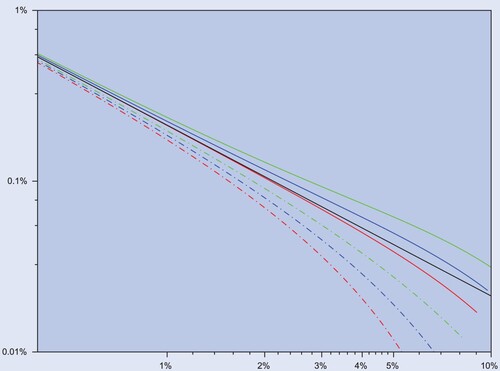
Figure displays the optimal trading boundaries against tracking error: low tracking error (left, corresponding to high γ) implies a narrow no-trade region, and thus frequent rebalancing. This regime is the most relevant for leveraged ETFs, as the users of these funds are primarily short-term traders, for whom the precise replication of daily returns is more important than average performance (Cheng and Madhavan Citation2009).
Figure 1. Buy (dashed) and sell (solid) boundaries (vertical, as risky weights π) versus average tracking error (horizontal) for leveraged (top) and inverse (bottom) funds, with multipliers 4 (top), 3, 2,
,
,
(bottom). As aversion to tracking error γ decreases from left (
) to right (
), for inverse funds (bottom) the trading boundaries widen around the target, whereas for leveraged funds (top) they first widen and then collapse to one.
and zero risk premium.
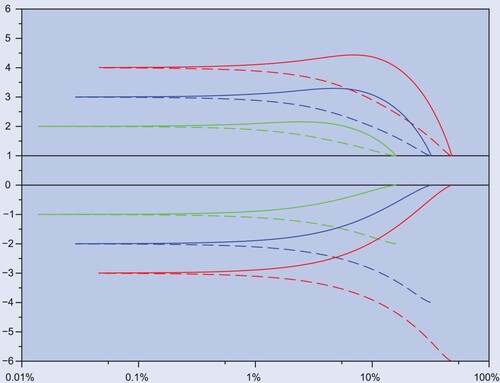
As the aversion to tracking error decreases (right), the priority shifts to reducing long-term average rebalancing costs, at the expense of higher tracking error. For leveraged funds, widening the no-trade region serves this purpose—up to a point. As the emphasis on low trading costs dominates, it becomes virtually impossible for a leveraged fund to track its target: the next best alternative is to closely replicate the index, which can be done essentially for free.
For inverse funds the situation is different: the closest factor that is replicable at no cost is zero, therefore the no-trade region continues to widen until its sell boundary becomes exactly zero, while remaining symmetric around its target multiple to preserve pre-existing short positions. At that point, negative exposure is seldom decreased (at the buy boundary, for the sake of solvency) and never increased (as the sell boundary of zero is never reached).
Overall, the small tracking errors that are typically sought by managers of leveraged and inverse funds lead to similar replication strategies, based on nearly symmetric no-trade regions. Excessive emphasis on small costs would break this symmetry: because the only costless multiples are zero and one, leveraged funds would veer toward one, while inverse funds would veer toward preservation of negative exposure while retaining solvency.
3.2. Tracking difference versus tracking error
Figure displays in log scale the tradeoff between tracking difference and tracking error for funds with different factors. For small trading costs, (Equation21(21)
(21) ) implies that this tradeoff is approximately
which corresponds to the negative, approximately linear dependence in the left of the graphs. As the right-hand side remains constant if Λ is replaced by
, for small tracking error a
inverse fund faces a tradeoff similar to the one of a leveraged fund with factor Λ. Put differently, a
leveraged fund is as difficult to manage as a
inverse fund. This is clear from the comparison of solid and dashed lines with same color in the figure.
Figure 2. Negative tracking difference (, vertical) against tracking error (horizontal) for leveraged (solid) and inverse (dashed) funds, in logarithmic scale, from −3, +4 (top), to −2, +3 (middle), and −1, +2 (bottom). As aversion to tracking error γ decreases from left (
) to right (
), a k + 1-leveraged fund is akin to a
inverse one, as the respective curves (same color) approach low and high
aversion.
,
, and zero risk premium.
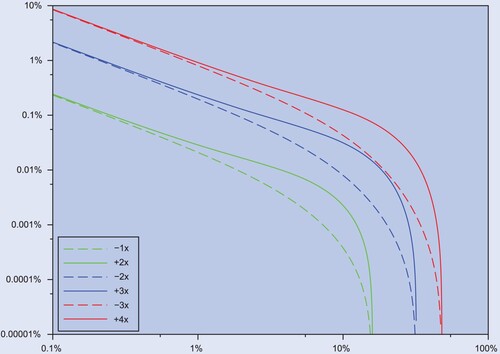
As tracking error increases, the inverse fund's tradeoff improves, in that its optimal policy yields a less negative tracking difference than the symmetric leveraged fund because the boundaries of inverse funds keep widening even as those of leveraged funds start shrinking. As the tracking error increases further, their performances become again trivial, as both leveraged and inverse exposures are allowed to depart from their targets to avoid trading costs.
3.3. Implied spread
Equation (Equation21(21)
(21) ) links the tracking difference, tracking error, leverage factor, index volatility, and trading spread ε. As the tracking error represents the standard deviation of the estimate of the tracking difference
, a low tracking error means that in this equation all quantities are estimated accurately, with the exception of the spread ε. In principle, one could estimate ε as the average bid-ask spread observed in the index, but in practice such an estimate would overstate the rebalancing costs of leveraged and inverse funds, as they achieve their index exposure primarily through total return swaps and futures, which offer much lower trading costs than the index components. In practice (cf. section 4), direct holdings of the index' components are typically less than the fund's assets for leveraged funds and are actually zero for inverse funds (i.e. there are no short positions in index' components but only in swaps and futures).
This observation suggests to use (Equation21(21)
(21) ) to define the implied spread as
in a similar way as the familiar Black–Scholes formula is used to define implied volatility rather than to price options. The implied spread offers a more attractive measure of the fund's performance than the tracking difference or the tracking error, as it controls for the effects of both volatility and the leverage factor.
This definition measures the trading cost, above which the investor is better off replicating the fund's payoff by trading, and below which the fund offers a cheaper alternative. The theoretical (population) spread is always positive, as the corresponding tracking difference is necessarily negative in view of trading costs. However, sample estimates can and do lead to occasionally negative implied spreads, which materialize if the fund deviates from a close replication, and happens to outperform its target by mere chance. In fact, such imprecise estimates of the implied spread result from the imprecise estimates of the tracking difference when the tracking error is large.
In summary, the implied spread offers a synthetic figure that represents the cost for investors of leveraged and inverse funds, adjusting for the effects of the factor, volatility, and the tradeoff between tracking error and tracking difference. However, such a measure is accurate only when the tracking difference is accurate, which is when the tracking error is sufficiently low.
3.4. R-Squared
The squared correlation of a fund's return with its benchmark is an intuitive, scale-free statistic, which reflects the fraction of the fund's variance that is explained by the benchmark's own variance. For funds with relatively low factors, such as the ones traded in US markets, the squared correlation is similarly close to the frictionless level of 100%, leaving few insights to be gleaned from this quantity.
Equations (Equation15(15)
(15) ) and (Equation20
(20)
(20) ) provide respectively the exact and asymptotic formulas of squared correlation. Importantly, the
does not depend on the volatility process, but only on the trading cost ε, the leverage factor Λ, and the aversion parameter γ that controls the tradeoff between tracking difference and tracking error. Figure plots the squared correlation against the leverage factor, highlighting several effects. First, squared correlation declines for large positive and negative factors, as the optimal no-trade region widens and the fund's exposure is increasingly variable.
Figure 3. Exact (vertical) for inverse and leveraged factors Λ (horizontal), with aversion parameter
(blue) and
(green).
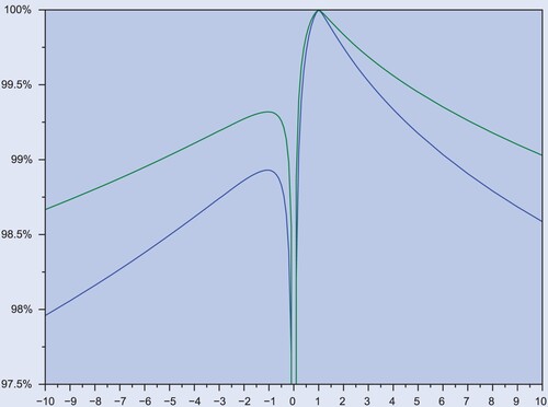
Second, squared correlation is asymmetric in the factor and systematically lowers for inverse funds. For positive factors, correlation is poor near zero, becomes perfect at the benchmark value of one, and deteriorates as leverage increases further. As negative factors do not include the benchmark, their correlation is generally lower, and achieves its maximum near minus one.
The low correlation near the zero factor, though empirically irrelevant, deserves a comment, in view of its differences with the factor of 1. The explanation of such low correlation is that a fund with near-zero exposure combines a very low volatility with a relatively wide no-trade region, resulting in a fund's exposure that is rather variable, and poorly explained by the benchmark's return.
There are two extreme cases, , which are explicitly excluded in theorem 3.1. In these cases, an optimal trading policy is not to engage in trading at all; thus both transaction costs and tracking error vanish. Therefore, the tracking error cannot be freely chosen, as the value function vanishes and the optimal policy is independent of the value of γ.
Indeed, equations (Equation13(13)
(13) ), (Equation14
(14)
(14) ) and (Equation15
(15)
(15) ) imply the relation between
and tracking error
which yields the asymptotic formula
This formula validates the usual interpretation of
as fraction of variance in the fund unexplained by the variation in the benchmark and shows that for Λ near zero even a small but positive tracking error can lead to a low
, as the factor Λ appears in the denominator.
4. Replication of LIETFs
The model in this paper relies on the assumption that trading costs incurred by fund managers are a small constant proportion of amounts traded. Thus it is opportune to investigate the relevance of such an assumption for the replication of LIETFs.
Engle et al. (Citation2012) estimate average transaction costs of 8.8 and 13.8 basis points (bps) for NYSE and NASDAQ respectively, based on orders executed by Morgan Stanley in 2004. Their estimates for trading cost rise to 27 bps for relatively larger orders—higher than 1% of the stock's daily trading volume. Similarly, Frazzini et al. (Citation2012) estimate median transaction cost of 4.9 bps, with a value-weighted average of 9.5 bps, which reflect the higher cost of larger trades. In short, empirical studies suggest that trading costs are near 0.1%, except for orders that are higher than 1% of daily trading volume. Thus, to evaluate whether the assumption of constant trading costs is appropriate, it is necessary to understand (i) the details of the rebalancing strategies of leveraged and inverse ETFs and (ii) the relative size of their trading volume compared to that in the underlying index.
To investigate rebalancing strategies, we obtained from ProShares the daily holdings at the security level of the main leveraged and inverse ETFs on the S&P 500 index from January 26 to April 6, 2018. This period included a number of days with large market movements, which offer the opportunity to observe rebalancing behavior in volatile times. Because the institutional objective of these funds is to offer a multiple of the daily return on the underlying index, the daily frequency is the natural one to study rebalancing. It is also the highest frequency for which public data are available.
Note also that LIETFs trade both to rebalance in response to the index' return, and to adjust exposure in response to the creation and redemption of shares by authorized participants. Thus the index return alone is not a reliable indicator of the trading volume. Instead, the direct inspection of daily portfolio composition reflects the overall trading volume resulting from both managers' rebalancing and investors' flows.
The left panel in table shows the source of exposure to the index for each of the S&P 500 funds: most of the exposure is achieved through index swaps contracts with various counterparties (such as Goldman Sachs, Bank of America, JP Morgan, Credit Suisse, and other financial institutions). Such contracts are typically multiples of 10 or 100 million USD and are rebalanced in such multiples. A small fraction of the exposure is achieved through E-mini futures contracts on the S&P 500. For leveraged funds, a substantial amount of exposure, approximately 80% percent of the fund's assets, is achieved through direct ownership of each of the 505 index' components. By contrast, inverse funds do not take short positions in the index' components, thereby avoiding short sale costs associated with borrowing shares of individual stocks, while achieving exposure entirely through swaps and futures.
Table 1. Average exposure (left) and average daily turnover (right), both as percent of funds' values, in different asset classes for S&P 500 LIETFs: SPXU (−3), SDS (−2), SH (−1), SSO (+2), UPRO (+3), from 2018-01-26 to 2018-04-06.
Comparing the changes in each security's daily holdings over time reveals the magnitude of the trading amounts generated by ProShares funds on the S&P 500 index. The right panel in table displays the average daily turnover for each factor and asset class as a percentage of the fund's assets. As observed in the introduction, the overall turnover is significantly higher for larger negative factors, with the factor generating approximately twice as much turnover as
or 3. In addition, the table reveals that in practice most of the turnover is concentrated in index swaps, with a significant minority of trading in futures and, for positive factors, in stocks. Such a pecking order reflects the lower trading costs of index swaps relative to futures and of futures relative to stocks.
To understand the size of trading volume in LIETFs compared to trading volume in the index, we examined daily assets under management for all the Proshares funds on the S&P 500 index since June 23, 2009, the first day on which all funds multiples are available. This information allows to compute the total volume generated by all funds, both from rebalancing and from the subscription or redemption of shares. Comparing such daily volume to the total volume generated by trading in the stocks included in the S&P 500 index, yields for each day the ratio between ETFs volume and stock market volume. The summary statistics are in table : trading volume generated by LIETFs activity averages approximately 0.20% of trading volume in the S&P 500 index components, and on 99 out of 100 days it is below 0.86%.
Table 2. Summary statistics for the ratio (as percent) between (i) daily volume generated by LIETFs on the S&P 500 and (ii) daily volume in the S&P 500 components. Data from 2009-06-23 to 2018-03-27.
These figures imply that, even in the implausible worst case scenario that all trading generated by LIETFs took place in underlying assets, such volume would be on average five times below the 1% threshold above which price impact starts to become relevant. In practice, as shown by table , only a minority of trading takes place in the underlying assets, with the bulk concentrated in index swaps and futures, which entail much lower trading costs, thereby indicating that the assumption of constant trading costs is germane to the present application.
5. Empirical results
This section examines the model's implications for leveraged and inverse exchange-traded funds listed in the USA.
Table displays the performance statistics for some of the largest families of leveraged and inverse ETFs. To facilitate comparisons among different factors of the same benchmark, observations for each family are trimmed to the longest period that includes all factors (the youngest funds are usually the ones with triple exposure). Each row displays the relative performance of a leveraged or inverse fund compared to a hypothetical portfolio that trades without costs in the nonlevered fund on the same benchmark (e.g. SPY before management fees for the S&P 500), using as safe rate the 1-month treasury rate. The beta and tracking differences are calculated from the linear regression of the fund's daily returns on the returns of the corresponding hypothetical portfolio.
Table 3. Performance of LIETFs on selected indexes through December , 2022. For each index, observations begin on the earliest date for which all inverse (−3, −2, −1) and leveraged (2, 3) multiples are available. (Earliest date is November
, 2008.) Historical prices from Yahoo Finance, Interest rates from US Treasury.
Average exposures (betas) are closely aligned with their targets, but consistently biased towards zero, and such differences are statistically significant for higher factors, as documented by their t-statistics. This is the underexposure puzzle, observed by Tang and Xu (Citation2013), and explained in our model by equation (Equation22(22)
(22) ) as the result of optimal rebalancing policies. The higher tracking error of funds with larger factors follow from the wider no-trade regions that are optimal for larger factors. Likewise, more negative tracking differences for larger factors may reflect higher rebalancing costs rather than management issues.
The implied spreads in table tend to be lower for larger factors ( than they are for smaller ones
. In other words, the tracking differences of a larger factor is less negative than it should be if the spread was the same as for smaller factors. Such differences are large, ranging from around 5 basis points for larger factors to about 20 for small factors.
An explanation of this difference is in the relatively flat management fees charged by funds with different factors: for example, the funds that replicate multiples of the S&P 500 index have expense ratios of 0.90% (−3), 0.90% (−2), 0.89% (−1), 0.89% (+2), and 0.91% (+3). These expenses detract directly from the tracking difference of the fund, and make it much more onerous for an investor (in terms of implied rebalancing cost) to pay for a fund that generates twice the index return, than to pay
for three times. For inverse funds it is even more obvious, as the once and twice inverse funds have virtually the same expenses.
The relevance of this explanation is further confirmed by the gross implied spreads, that is, the implied spreads obtained by the tracking differences before management fees (obtained in the data by adding to the market return the daily management fee of the fund). In accordance with the above explanation, such gross implied spreads are significantly closer to each other across different factors. Some of the gross spreads for the most liquid funds take small negative values due to the effect of tracking error, as the realized return in the sample period is minimally positive before fees.Footnote11 Consistently with the model, gross implied spreads are higher for less liquid asset classes, such as smaller stocks (S&P Midcap 400 and Russel 2000).
In summary, while the gross implied spread is useful to understand the impact of management fees and managers' tracking efficiency, the relevant performance measure for investors is the net implied spread, as it captures the only return that is available to them, i.e. net of fees.
5.1. Underexposure
In their empirical work on leveraged and inverse ETFs listed in US exchanges, Tang and Xu (Citation2013) report that ‘LETFs show an underexposure to the index that they seek to track’. That is, empirical average exposures are significantly closer to zero than their target multiple. Table confirms the underexposure phenomenon for several families of leveraged and inverse ETFs traded in US markets: the comparison of realized average exposure with target factors yields significant t-statistics for the riskiest funds, with deviations consistently biased toward zero.
This empirical regularity is explained by equations (Equation14(14)
(14) ) and (Equation19
(19)
(19) ) as a consequence of managers' optimal rebalancing policies. Indeed, the transaction cost correction in
(22)
(22)
is negative for
and positive for
. This effect may seem puzzling at first, as the buy and sell boundaries are approximately symmetric around Λ.
The crucial point is that when the exposure is larger (farther from zero), it is also more variable. As the trading policy forces exposure to remain in a fixed range, the implication is that, within such range, the exposure on average spends more time on less variable values—where it is closer to zero. Thus the underexposure effect arises from the combination of symmetric trading boundaries with the asymmetric volatility of the fund.
Substituting in equation (Equation22(22)
(22) ) a fund's average realized exposure as
, it is possible to solve for the ratio
, which, combined with a value of the trading cost ε, yields an estimate for γ. Larger deviations of the average exposure
from the target factor Λ imply a lower γ (the manager favors lower trading costs over lower tracking error) while smaller deviations imply a larger value of γ.
For example, the SPXU has a realized and a factor
, which imply
assuming that
, a figure consistent with the discussion in the previous section. Table displays the average exposure implied for funds with typical factors for different values of ε and γ. Small factors (
and 2) lead to average exposures that are almost indistinguishable from their targets, especially when statistical error is accounted for. On the other hand, larger factors (
,
, and 3) lead to discernible differences across
aversion γ and trading costs ε. In particular, the configuration
closely approximates the panel of S&P 500 funds and
the panel of Dow Jones funds. In general, values of γ between 5 and 10 with
closely reproduce the empirical estimates on funds tracking large-capitalization stocks, while higher trading costs ε are warranted for small-capitalization stocks and treasuries.
Table 4. Average exposure () for typical factors (Λ) across trading costs (ε) and
aversion (γ), obtained from equation (Equation22
(22)
(22) ).
Granularity
It is worthwhile to consider whether the observed underexposure may have different explanations. One ostensible source of underexposure could be granularity. Indeed, the minimum trade size for the E-mini S&P 500 Futures contract (which is held by the ETFs tracking this index, as explained in the previous section) equals $50 times the index value, which means that when the index is 2800, the contract size is $140,000. Thus for a fund with a $1 billion exposure (the SSO has more than 2 billion in assets, hence an exposure of over 4 billions), the granularity of futures contracts could explain a discrepancy in average exposure of the order of .
In fact, the inspection of daily portfolio holdings described above reveals that, because daily rebalancing of leveraged (but not inverse) funds is partly achieved by trading incremental quantities of individual equities, the minimum trade unit for a fund is the price of one share, typically between $10 and $1000. Thus, for a fund with $1 billion exposure, the granularity of equity prices could justify a discrepancy in average exposure of the order of . Note also that granularity—whether from futures contract sizes or equity prices—would generate either underexposure or overexposure with comparable probabilities.
Empirically, the underexposure observed even for the largest ETFs, with assets under management above $1 billion, is of the order of , while overexposure never appears in any of the 40 funds in our original sample. Taken together, these observations indicate that granularity does not reproduce quantitatively the observed underexposure of major leveraged and inverse exchange-traded funds.
Noisy Returns
Another potential source of underexposure is measurement error in the returns of LIETFs and their underlying index. For example, such an error can arise if such returns are calculated from net asset values (NAVs) rather than market prices, which differ slightly from NAVs, due to time lags in their calculation and to small deviations, within the cost of subscription and redemption, which cannot be arbitraged away.
Thus, denote the observed return of a fund as , where
is the true return and
is a measurement error and, likewise, the observed return of the underlying index as
. Then, assuming that returns are stationary and that errors are uncorrelated with true returns and with each other, the large sample average exposure converges in probability to
where
is the true average exposure. In other words, measurement error in the fund's return does not bias the estimate of average exposure, but measurement error in the index' return generates a spurious proportional underexposure of
.
Note that such underexposure is independent of the true or observed fund returns, and in particular it would be independent of the leverage factor, while the underexposure observed in table is much bigger for larger factors. This qualitative observation already casts doubt on such mechanism as a source of the observed underexposure. (In addition, the results in table do not rely on NAVs but on market prices only.)
A detailed analysis of returns of NAV and market prices sheds additional light on this issue. Indeed, for the SPY, which replicates the S&P 500 index, the standard deviation of the difference between daily NAV returns and market returns is 0.16%, while the standard deviations of both the market and the NAV daily returns are 1.15%, which implies that
(The observation period is 2003-12-02 to 2018-12-31.) Put differently, a measurement error equivalent to the discrepancy between NAV and market price would generate a reduction in average exposure of nearly 2%, irrespective of the factor considered. By contrast, the underexposures in table are much smaller for small factors, as NAVs are never used in the analysis.
The above observation helps understand why the underexposures reported here are smaller than the ones observed by Tang and Xu (Citation2013). Indeed, they calculate average exposures of LIETFs with respect to the underlying indexes rather than the market return of the nonlevered fund on the same index (this paper's approach). The benchmark index (which is not itself traded) may exhibit deviations from the market price of the same order as the NAV, and in fact Tang and Xu (Citation2013, table 1 B) report for the SPY an exposure of 98.48%, i.e. an underexposure of 1.52%, which is broadly consistent with the effect of noisy returns.
6. Robustness
This section discusses, theoretically and numerically, the robustness of previous results to risk premia with stochastic volatility, finite horizons, and discrete (as opposed to continuous) trading.
6.1. Risk premia: trading strategies and performance
Assume that the underlying S has non-zero risk premia,
where
, with
. Thus this specification prescribes that the Sharpe ratio increases as return variance increases, as in the asset pricing models of Campbell and Cochrane (Citation1999), Bansal and Yaron (Citation2004), and others, and consistent with the empirical countercyclicality of risk premia.
In view of the excess returns , the cumulative returns process
defined by (Equation4
(4)
(4) ) includes a component
that can be ascribed to the deviation of the fund's exposure from its target. As the exposure
is observable to investors,Footnote12 they can accordingly control for overexposure while evaluating performance, by modifying the definition of the deviation process as
(23)
(23)
Replacing (Equation4
(4)
(4) ) with (Equation23
(23)
(23) ), the previous identities (Equation5
(5)
(5) )–(Equation6
(6)
(6) ) for Tracking Difference (
) and Tracking Error (
) remain valid, and thus the objective of a leveraged ETF manager is to find a trading policy
that minimizes the average equivalent expense ratio
over all
, where Φ is the set of admissible strategies (see appendix 1). Note that in this problem, although the objective function controls for extra exposure, the risk-premium κ has not disappeared completely, as it affects the dynamics of the portfolio weight
. The question is whether this effect is significant enough to alter the previous results.
The next theorem offers a negative answer, in which the effect of the risk premium is found to be of the second order:
Theorem 6.1
(Risk Premia)
Let and
. For
small enough:
The free boundary problem
The trading strategy
The trading boundaries
The minimum Equivalent Expense Ratio is
Thus the risk premium κ affects the optimal trading boundaries only in the term, which is negligible for reasonable parameter values, as illustrated by figure . Similarly, the tracking difference and the average exposure of the fund are also affected at the second order. In particular, the performance formula (Equation21
(21)
(21) ) remains valid, as it involves only first-order terms.
Figure 4. Trading boundaries (vertical) for factor against tracking error (horizontal), from first-order asymptotics (Equation25
(25)
(25) ) (red) and exact solutions for
(black),
(blue), and
(green). For realistic levels of tracking error, the impact of κ is of second order.
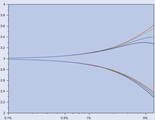
On the issue of performance, figure reproduces the relevant part of figure with realistic risk premia. Again, the main message is that the tradeoff between tracking error and tracking difference remains virtually unchanged at typical levels of tracking error and target factors.
Figure 5. Negative tracking difference () for
leveraged fund (vertical, colored solid lines) and
(dashed colored lines), against tracking error (TrE) (horizontal), for
(black),
(blue) and
(green). The solid red line represents the asymptotic formula in (Equation1
(1)
(1) ), which is the same for L and 1−L.
6.2. Finite horizons, trading frequency, and stochastic volatility
The use of a stationary objective raises the question of how robust the results are to fixed horizons, and how well stationary optimal strategies perform when trading takes place at discrete frequency, rather than continuously. Figure plots the asymptotic tradeoff between tracking difference and tracking error to the one obtained from Monte Carlo simulations from geometric Brownian motion (Black–Scholes model) and from the Heston stochastic volatility model, in the presence of a risk premium, with daily rebalancing frequency, and for a finite horizon of 5 years.
Figure 6. Negative tracking difference () for a
leveraged fund (vertical), against tracking error (horizontal), for
(solid lines), 1.5625 (dashed) and 3.125 (dashed-dotted), when
. The black lines depicts the exact performance from (Equation26
(26)
(26) ) with
. The blue and green lines correspond to Monte Carlo Estimates (15000 paths, daily grid) for the Black–Scholes (blue) and Heston (green) models, with time horizon of T = 5 years, daily sampling and trading frequency, and correlation
.
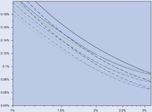
For the Heston model, set , where
satisfies the dynamics
with an instantaneous correlation
, and the parametrization
,
, unconditional mean
, mean-reversion speed
and diffusion coefficient σ. A minimal trade is executed whenever the proportion of wealth π leaves the no-trade region
as to return π to its closest boundary. The exact trading boundaries
are obtained by solving numerically (Equation24
(24)
(24) ) subject to the free boundary conditions (Equation10
(10)
(10) )–(Equation11
(11)
(11) ).
Again, the message of figure is that, for realistic parameter values, risk premia, trading frequencies, and finite horizons have only a minor effect on the basic tradeoff identified by the asymptotic formulas in the paper. While these features make the optimization problem more complex, they remain largely inconsequential for performance evaluation and replication purposes.
7. Conclusion
Leveraged and inverse funds seek to replicate a multiple of the daily return on an index by frequently rebalancing their portfolio to keep a constant leverage ratio. In theory, in a frictionless market continuous rebalancing yields a perfect replication of a leveraged benchmark, i.e. zero alpha and tracking error. In practice, trading costs create a trade-off between the frequent rebalancing that generates low tracking error and the low trading costs that prevent alpha from becoming too negative. This trade-off becomes more relevant for products that seek to replicate larger multiples or less liquid benchmarks.
Portfolio performance measures based on the regression of a fund's return against its benchmark's return are ubiquitous, hence closely monitored by managers who may be evaluated on their basis. On average, the negative tracking difference of a leveraged fund results from management fees and trading costs, while the tracking error reflects the inevitable deviations from the target exposure that are necessary to keep trading costs under control. Other things equal, a fund that seeks to replicate a larger multiple of an index' return has a higher tracking error and a more negative tracking difference.
It is misleading to compare funds with different factors, and to conclude that one is better managed than the other merely because its tracking error is lower, or because its alpha is less negative: two funds with the same factor may be optimally managed, as one may seek lower tracking error at the expense of more negative tracking difference. High tracking error is not necessarily evidence of poor manager performance if the index is less liquid. On the contrary, a savvy management strategy must accept higher tracking error to achieve less negative tracking differences, and low tracking error inevitably depresses average performance.
Open Scholarship
This article has earned the Center for Open Science badges for Open Data and Open Materials through Open Practices Disclosure. The data and materials are openly accessible at https://github.com/guasoni/leveraged-funds/.
Acknowledgments
For helpful comments, we thank Michael Brennan, Doug Breeden, Lisa Goldberg, Tim Leung, Johannes Muhle-Karbe, Mathieu Rosenbaum, Ronnie Sircar, Matt Spiegel, Renè Stulz, Peter Tankov and seminar participants at University of Vienna, London School of Economics, Johns Hopkins University, Séminar Bachelier Paris, University of Warwick, the 9th Financial Risks International Forum (Paris), and the Byrne Workshop at the University of Michigan. A special thanks to the anonymous referee, who helped improve the interpretation of figure .
Data Availability Statement
The code and data supporting this paper's findings are at https://github.com/guasoni/leveraged-funds.
Disclosure statement
No potential conflict of interest was reported by the authors.
Additional information
Funding
Notes
1 These figures exclude other leveraged and inverse exchange-traded products such as exchange-traded notes, which have significantly different characteristics.
2 See https://www.sec.gov/news/pressrelease/2015-276.html and https://www.wsj.com/articles/sec-reconsidering-staff-approval-of-first-quadruple-leveraged-etf-1494970106.
3 A fund with factor Λ generates a daily turnover of times the index return (Cheng and Madhavan Citation2009).
4 The website https://www.trackingdifferences.com/ publishes the tracking differences of ETFs listed in several exchanges.
5 See Magill and Constantinides (Citation1976), Constantinides (Citation1986), Taksar et al. (Citation1988), Davis and Norman (Citation1990), Dumas and Luciano (Citation1991), and the asymptotic results in Shreve and Soner (Citation1994), Rogers (Citation2004), Gerhold et al. (Citation2014), Kallsen and Muhle-Karbe (Citation2017), and Melnyk and Seifried (Citation2018).
6 Cf. Cheng and Madhavan (Citation2009), Jarrow (Citation2010), Avellaneda and Zhang (Citation2010), and Lu et al. (Citation2012).
7 The convention of evaluating the risky position at the ask price is inconsequential. Using the bid price instead leads to the same results up to a change in notation.
8 Both limits hold in probability. The first convergence follows by the continuity of D, and the second one from theorem IV.1.3 in Revuz and Yor (Citation1999) by localization.
9 The equality follows from lemma A.2, see also Remark A.3.
10 This quantity is well defined by virtue of assumption 2.1, which guarantees that tracking error does not diverge. The lim inf guarantees a good definition a priori. A posteriori, optimal strategies exist in which the limit inferior is a limit, hence the similar problem defined in terms of lim inf has the same solution. Note also that, if volatility σ is a function of some stationary Markov process, the first term in (Equation8(8)
(8) ) is equivalent to
, where the random variable Y has the stationary distribution under the expectation
. In particular, the formulation in (Equation7
(7)
(7) ) in terms of a time-average is equivalent to a direct ergodic formulation of the problem. We keep the current formulation because it is does not involve the Markov property and because an ergodic formulation of the trading cost in (Equation8
(8)
(8) ) would require the use of local times as well as further restrictions on trading strategies.
11 The notable exception is the EET, which has a large negative tracking difference and hence a large implied spread, even after controlling for management fees.
12 Note that and
, whence
.
13 are increasing processes (therefore, if
, then L, U are decreasing).
14 Note that in the present setting, equation (EquationA27(A27)
(A27) ) generalizes to
but in view of the logarithmic term (
), it is not tractable and therefore abandoned. (We therefore invoke in this section optimality of the trading strategy associated with the boundaries
,
, cf. remark A.12).
References
- Anderson, R.M., Bianchi, S.W. and Goldberg, L.R., Will my risk parity strategy outperform? Financial Anal. J., 2012, 68(6), 75–93.
- Anderson, R.M., Bianchi, S.W. and Goldberg, L.R., Determinants of levered portfolio performance. Financial Anal. J., 2014, 70(5), 53–72.
- Avellaneda, M. and Zhang, S., Path-dependence of leveraged ETF returns. SIAM J. Financial Math., 2010, 1(1), 586–603.
- Bansal, R. and Yaron, A., Risks for the long run: A potential resolution of asset pricing puzzles. J. Finance, 2004, 59(4), 1481–1509.
- Campbell, J.Y. and Cochrane, J.H., By force of habit: A consumption-based explanation of aggregate stock market behavior. J. Econom. Theory, 1999, 107(2), 205–251.
- Carr, P. and Madan, D., Towards a theory of volatility trading. In Option Pricing, Interest Rates and Risk Management, Handb. Math. Finance, pp. 458–476, 2001 (Cambridge University Press: Cambridge).
- Charteris, A. and McCullough, K., Tracking error vs tracking difference: does it matter? Investment Anal. J., 2020, 49(3), 269–287.
- Cheng, M. and Madhavan, A., The dynamics of leveraged and inverse exchange-traded funds. J. Investment Manag., 2009, 16(4), 43.
- Constantinides, G., Capital market equilibrium with transaction costs. J. Polit. Economy, 1986, 94(4), 842–862.
- Dai, M., Kou, S., Soner, H.M. and Yang, C., Leveraged exchange-traded funds with market closure and frictions. Manage. Sci., 2022, 69(4), 2517–2535.
- Davis, M.H.A. and Norman, A.R., Portfolio selection with transaction costs. Math. Oper. Res., 1990, 15(4), 676–713.
- Dumas, B. and Luciano, E., An exact solution to a dynamic portfolio choice problem under transactions costs. J. Finance, 1991, 46(2), 577–595.
- Dupire, B., Model art. Risk, 1993, 6(9), 118–124.
- Engle, R., Ferstenberg, R. and Russell, J., Measuring and modeling execution cost and risk. J. Portfolio Manag., 2012, 38(2), 14–28.
- ESMA, Guidelines for competent authorities and units management companies: Guidelines on ETFs and other UCITS issues, 2014. European Securities and Markets Authority. https://www.esma.europa.eu/sites/default/files/library/2015/11/esma-2014-0011-01-00_en_0.pdf.
- Frazzini, A., Israel, R. and Moskowitz, T.J., Trading costs of asset pricing anomalies. Fama-Miller Working Paper, 14–05, 2012.
- Frino, A. and Gallagher, D.R., Tracking S&P 500 index funds. J. Portfolio Manag., 2001, 28(1), 44–55.
- Gerhold, S., Guasoni, P., Muhle-Karbe, J. and Schachermayer, W., Transaction costs, trading volume, and the liquidity premium. Finance Stoch., 2014, 18(1), 1–37.
- Guasoni, P. and Mayerhofer, E., The limits of leverage. Math. Finance, 2019, 29(1), 249–284.
- Gunning, R.C. and Rossi, H., Analytic Functions of Several Complex Variables, Vol. 2009 (American Mathematical Society).
- Jarrow, R.A., Understanding the risk of leveraged ETFs. Finance Res. Lett., 2010, 7(3), 135–139.
- Johnson, B., Bioy, H., Kellett, A. and Davidson, L., On the right track: measuring tracking efficiency in ETFs. J. Index Investing, 2013, 4(3), 35–41.
- Kallsen, J. and Muhle-Karbe, J., The general structure of optimal investment and consumption with small transaction costs. Math. Finance, 2017, 27(3), 659–703.
- Lu, L., Wang, J. and Zhang, G., Long term performance of leveraged ETFs. Financial Services Rev., 2012, 21(1). https://go.gale.com/ps/retrieve.do?tabID=T002&resultListType=RESULT_LIST&searchResultsType=SingleTab&retrievalId=8f6fb502-7809-4a00-90cf-f06b2d717375&hitCount=6&searchType=AdvancedSearchForm¤tPosition=6&docId=GALE%7CA309587934&docType=Report&sort=Relevance&contentSegment=ZONE-Exclude-FT&prodId=AONE&pageNum=1&contentSet=GALE%7CA309587934&searchId=R2&userGroupName=anon%7E61bbbbab&inPS=true.
- Magill, M.J.P. and Constantinides, G.M., Portfolio selection with transactions costs. J. Econom. Theory, 1976, 13(2), 245–263.
- Melnyk, Y. and Seifried, F.T., Small-cost asymptotics for long-term growth rates in incomplete markets. Math. Finance, 2018, 28(2), 668–711.
- Neuberger, A., The log contract. J. Portfolio Manag., 1994, 20(2), 74–80.
- Revuz, D. and Yor, M., Continuous Martingales and Brownian Motion, 3rd ed., 1999 (Springer: Berlin).
- Rogers, L.C.G., Why is the effect of proportional transaction costs O(δ2/3)? In Mathematics of Finance, Vol. 351 of Contemp. Math., pp. 303–308, 2004 (American Mathematical Society: Providence, RI).
- Shreve, S.E. and Soner, H.M., Optimal investment and consumption with transaction costs. Ann. Appl. Probab., 1994, 4(3), 609–692.
- Taksar, M., Klass, M.J. and Assaf, D., A diffusion model for optimal portfolio selection in the presence of brokerage fees. Math. Oper. Res., 1988, 13(2), 277–294.
- Tang, H. and Xu, X.E., Solving the return deviation conundrum of leveraged exchange-traded funds. J. Financial Quant. Anal., 2013, 48(1), 309–342.
- Wagalath, L., Modelling the rebalancing slippage of leveraged exchange-traded funds. Quant. Finance, 2014, 14(9), 1503–1511.
Appendices
Appendix 1. Admissible Trading Strategies
Definition A.1
A non-anticipative, self-financing strategy (compare (Equation2(2)
(2) )–(Equation3
(3)
(3) )) is admissible if it is solvent and satisfies sufficient integrability:
its liquidation value is strictly positive at all times: There exists
Let
The family of admissible trading strategies is denoted by Φ.
Let be the safe position of an admissible, self-financing trading strategy φ, and
the risky position. The following lemma describes the dynamics of the fund value
, the risky weight
, and the risky/safe ratio
.
Lemma A.2
Let φ be an admissible trading strategy, then
(A2)
(A2)
Moreover, the functional
can be written as
(A3)
(A3)
Proof.
The proof follows from similar arguments as in Guasoni and Mayerhofer (Citation2019, lemma A.2).
Remark A.3
Note that zero risk premia () imply
(as in this case
equals
in expectation, compare (Equation4
(4)
(4) )). Accordingly, the appendix (except part A) focuses on the equivalent problem of maximizing the functional
(A4)
(A4)
Appendix 2. Replication of Leveraged Benchmarks
This section contains a series of propositions, which culminate in a proof of theorem 3.1 in section 4. In particular, the optimal trading strategies are derived for replicating leveraged benchmarks under transaction costs. Setting
the free boundary problem (Equation9
(9)
(9) )–(Equation11
(11)
(11) ) can be recast as
(A5)
(A5)
(A6)
(A6)
(A7)
(A7)
For the next statement, the third root of a negative number a is understood as the unique real root of the equation
.
Proposition A.4
Let . For sufficiently small ε, the free boundary problem (EquationA5
(A5)
(A5) )–(EquationA7
(A7)
(A7) ) has a unique solution
, with
. The free boundaries have the asymptotic expansion
(A8)
(A8)
Proof.
Proof of proposition A.4
The differential equation (EquationA5(A5)
(A5) ) is equivalent to
As
, any solution of the initial value problem (EquationA5
(A5)
(A5) )–(EquationA6
(A6)
(A6) ) is thus of the form
By the terminal conditions (EquationA7
(A7)
(A7) ) at
, and setting
,
satisfy the system
(A9)
(A9)
(A10)
(A10)
The unique solution of the free boundary problem can be thus obtained by solving equations (EquationA9
(A9)
(A9) )–(EquationA10
(A10)
(A10) ). Moreover, expanding
around
with unknown coefficients
yields
Setting the relevant coefficients of the expansion to zero, it follows that
(A11)
(A11)
which yields
(A12)
(A12)
Finally, it is shown that equations (EquationA9
(A9)
(A9) )–(EquationA10
(A10)
(A10) ) have a unique solution around
This is equivalent to
having a unique solution
around
for sufficiently small δ. As
the Implicit Function Theorem for analytic functions (Gunning and Rossi Citation2009, theorem I.B.4) implies the existence of a unique solution. The higher order coefficients in (EquationA8
(A8)
(A8) ) are obtained similarly.
Proposition A.5
Let be the solution of the free boundary problem (EquationA5
(A5)
(A5) )–(EquationA7
(A7)
(A7) ) (provided by proposition A.4). For sufficiently small ε, the pair
defined by
is a solution of the HJB equation
(A13)
(A13)
Proof.
Proof of proposition A.5
First, recall that either (implying
) or
(implying
; thus for both ranges,
We show now the validity of (EquationA13
(A13)
(A13) ), by dividing the real line into the intervals parts
,
and
. For
, equation (EquationA5
(A5)
(A5) ) implies
and, the first initial condition in (EquationA6
(A6)
(A6) ) gives
whence
, for all
. Second, show
. As
(A14)
(A14)
if and only if
. Hence, either
, or
satisfies
. The first-order asymptotics of (EquationA8
(A8)
(A8) ) imply
for sufficiently small ε, and therefore
on
, and by (EquationA14
(A14)
(A14) ) it follows that
on all of
.
Third, note that on
. Indeed, the function
(see (EquationA9
(A9)
(A9) )) satisfies
hence for sufficiently small ε,
on some interval
, where
. Therefore, it suffices to show that
to verify the claim.
By contradiction, suppose there exists a sequence such that for each
, and that
. Changing to the variable
, and introducing the notation
,
shall prove convenient. By selecting, if necessary, a subsequence, one may without loss of generality assume that
converges, hence it must satisfy
, where
is defined in (EquationA12
(A12)
(A12) ), and
. The calculations leading to (EquationA12
(A12)
(A12) ) therefore entail that
must satisfy (EquationA11
(A11)
(A11) ) in place of
, i.e.
(A15)
(A15)
With
from (EquationA12
(A12)
(A12) ), the change of variable
implies
, which has the only solutions 1 and
. Therefore, (EquationA15
(A15)
(A15) ) has the only relevant solution
. Set
Then
satisfies
near
, for sufficiently small δ. By the uniqueness in the proof of proposition A.4,
, which contradicts the assumption
.
Consider now . As
, it suffices to show
Using
the asymptotic expansion (EquationA8
(A8)
(A8) ) implies
for sufficiently small ε. Furthermore,
, hence
for all
and for any sufficiently small ε.
Finally, consider . As
, only
needs to be checked. Note that L is a rational function and satisfies
, as
is a solution of the free boundary problem. Therefore it suffices to show L has no zeros on
, besides
. The transformation
,
leads to a rational function
, for which strict positivity has to be shown on
. As
, polynomial division by
yields
where g is a cubic polynomial. The further transformation
yields
, where
. Therefore
for all
and for any
, which translates into positivity of F, g and thus L.
Lemma A.6
Let be such that either
, or
or
. Then there exists an admissible trading strategy
such that the risky/safe ratio
satisfies SDE (EquationA2
(A2)
(A2) ). Moreover,
is a reflected diffusion on the interval
.
Proof.
See the first part of Guasoni and Mayerhofer (Citation2019, lemma B.5).
The following is the verification of optimality for the trading strategy of lemma A.6 with the trading boundaries in proposition A.4:
Proposition A.7
Denote by the trading strategy of lemma A.6 for the free boundaries
in proposition A.4, and let
Then for any t>0, the proportion of wealth
invested in the index lies in the interval
, almost surely, entails no trading whenever
, sells the index at
and buys it at
. The strategy
is optimal for sufficiently small ε, and the value function is
Proof.
Proof of proposition A.7
Recall from proposition A.5 that and
, defined from the unique solution of the free boundary problem, is a solution of the HJB equation (EquationA13
(A13)
(A13) ). For the verification, the proportion
of wealth in the index is used, instead of the risky/safe ratio
. With the change of variables
we introduce the operator
By proposition A.5 and the chain rule,
satisfies the HJB equation
(A16)
(A16)
for
, where
. By Itô's formula,
(A17)
(A17)
(A18)
(A18)
(A19)
(A19)
(A20)
(A20)
(A21)
(A21)
The first term in line (EquationA18
(A18)
(A18) ) is non-negative, due to (EquationA16
(A16)
(A16) ). Furthermore, by (EquationA1
(A1)
(A1) ) there exists
such that
, for all t, a.s.. Using (EquationA16
(A16)
(A16) ) one thus obtains
(A22)
(A22)
Hence, the integral (EquationA19
(A19)
(A19) ) is a martingale – in view of the integrability condition in assumption 2.1 – and has zero expectation. Furthermore, (EquationA16
(A16)
(A16) ) yields
which implies that for (EquationA20
(A20)
(A20) ) one has
Finally, (EquationA21
(A21)
(A21) ) is non-negative, because
due to (EquationA16
(A16)
(A16) ). Thus, taking the expectation of (EquationA17
(A17)
(A17) ) gives the estimate
(A23)
(A23)
By (EquationA22
(A22)
(A22) ),
therefore
Hence letting
in (EquationA23
(A23)
(A23) ) reveals that
for any admissible strategy φ. It is finally shown that this bound is attained by the admissible trading strategy
defined by lemma (A.6). Indeed, let
be the corresponding risky/safe ratio. Itô's formula yields
Integration with respect to t and division by T yields, in view of (EquationA3
(A3)
(A3) ),
Letting
, one obtains
.
Appendix 3. Performance Evaluation
While the trading strategies derived in the previous section are universal, in the sense that the trading boundaries are independent of (stochastic) volatility of the benchmark's returns, the various performance measures depend on the stationary volatility.
This section obtains explicit expressions for several moments related to the optimal trading strategy which allow in section 4 below to compute the performance statistics of theorem 3.1 are calculated in explicit form, in terms of the trading boundaries. Throughout the section, is the reflected diffusionFootnote13
(A24)
(A24)
on the interval
, where
, and where either
,
, or
. Accordingly, set
. Note that we do not require that
are optimal in the sense of theorem 3.1; it is only assumed that
to avoid bankruptcy.
The discussion begins with a lemma required in the proofs of several subsequent statements.
Lemma A.8
Let be an adapted process satisfying
. Then,
Proof.
Denote by for each
. The quadratic variation satisfies
which converges
a.s. to infinity as
(cf. Assumption 2.1). By the Dambis–Dubins–Schwarz Theorem,
, where
, is a Brownian motion on
and, by construction,
. Furthermore, as
is strictly increasing,
, hence
holds
a.s. Thus, by the law of iterated logarithm,
,
Proposition A.9
Let
(A25)
(A25)
Then the following
-a.s. limits hold:
(A26)
(A26)
(A27)
(A27)
(A28)
(A28)
Proof.
First, let , and
. Then Y is the reflected diffusion
on
. By lemma A.8,
and thus, by assumption (EquationA25
(A25)
(A25) ), equation (EquationA26
(A26)
(A26) ) follows. Furthermore, applying Itô's Formula to the function
yields
and in the limit, (EquationA27
(A27)
(A27) ) follows using lemma A.8 once again. Similar arguments yield (EquationA28
(A28)
(A28) ) using the function
and noting that
Lemma A.10
If
-a.s., then
(A29)
(A29)
Proof.
By (EquationA2(A2)
(A2) ) it follows that
and thus letting
, the first integral vanishes almost surely by lemma A.8. The remaining limits hold in view of assumption (EquationA25
(A25)
(A25) ).
A straightforward application of the preceding statements is the following:
Proposition A.11
For any (not necessarily optimal) trading strategy associated to (EquationA25
(A25)
(A25) ) is satisfied, and
-a.s.,
(A30)
(A30)
(A31)
(A31)
(A32)
(A32)
Remark A.12
This section does not assume that are the optimal trading boundaries of theorem 3.1. Invoking optimality, an alternative proof of proposition A.11 only requires the use of two of the four identities (EquationA26
(A26)
(A26) )–(EquationA29
(A29)
(A29) ).
Appendix 4. Proof of theorem 3.1
Proof.
The part (i) is covered by proposition A.4, and part (ii) is stated in proposition A.7. Part (iii) follows from proposition A.7 by using Remark A.3.
Proof of (iv) (Tracking Difference and Tracking Error): Let the optimal trading strategy defined by part (ii), and let
be the proportion of wealth in the risky asset. Recall the defining equation (Equation5
(5)
(5) ),
(A33)
(A33)
By lemma A.8, the first integral in (EquationA33
(A33)
(A33) ) vanishes almost surely, as
. Consider now the second term. Substituting
into (EquationA2
(A2)
(A2) ), the risky/safe ratio ζ satisfies equation (EquationA24
(A24)
(A24) ). Thus
and equation (EquationA30
(A30)
(A30) ) yields (Equation12
(12)
(12) ). As
formula (Equation13
(13)
(13) ) follows from equations (EquationA31
(A31)
(A31) )–(EquationA32
(A32)
(A32) ).
Proof of (v) (,
): The average volatility
of the optimal portfolio follows from (EquationA32
(A32)
(A32) ). Moreover, for fixed time horizons T the regression of
against
leads to the estimated slope, or beta, of this regression with the continuous-time approximation
According to equations (EquationA31
(A31)
(A31) )–(EquationA32
(A32)
(A32) ), the limit
(A34)
(A34)
is well defined. Similarly, the
of the regression, defined as the ratio between the variance of the predicted return and the variance of the realized return, is
(A35)
(A35)
Plugging equations (EquationA31
(A31)
(A31) )–(EquationA32
(A32)
(A32) ) into equations (EquationA34
(A34)
(A34) )–(EquationA35
(A35)
(A35) ) yields equations (Equation14
(14)
(14) ) and (Equation15
(15)
(15) ).
For part (vi), the asymptotic expansions of the trading boundaries , (Equation16
(16)
(16) ), follow directly from those for the free boundaries
in proposition A.4. Furthermore, (Equation16
(16)
(16) ) allows to calculate the respective expansions for EER,
,
, average volatility
, exposure
and
by using their explicit expressions in terms of
provided in theorem 3.1.
Appendix 5. Robustness
In the presence of excess returns (), the risky/safe ratio of any admissible trading strategy follows the dynamics
and thus the ODE of the free boundary problem is slightly modified to (Equation24
(24)
(24) ), but formulated with the same boundary conditions (Equation10
(10)
(10) )–(Equation11
(11)
(11) ). Similar proofs as those of theorem 3.1(i) carry over to all points of theorem 6.1. For the sake of completeness, we sketch the derivation of the free boundaries. The solution of (Equation24
(24)
(24) ) subject to the first boundary conditions (Equation10
(10)
(10) ) is of the form
Insisting on the terminal boundary conditions of zero and first order (Equation11
(11)
(11) ) results in the following system of equations for the free boundaries
,
,
For sufficiently small ε, we thus arrive at the asymptotic expansions
from which the asymptotics (Equation25
(25)
(25) ) of the trading boundaries
follow.
For figure , the exact tracking differences and tracking errors for the optimal trading strategies are used (see theorem 6.1(ii)). To obtain the corresponding formulas, we start with the following modificationFootnote14 of proposition A.9:
Lemma A.13
If
(A36)
(A36)
then the following limits hold
-a.s.:
(A37)
(A37)
(A38)
(A38)
The appropriate generalization of lemma A.10 is as follows:
Lemma A.14
If then
Proof.
Apply Itô's formula to the functional . All drift terms vanish. Division by T and letting
yields the claim (the Brownian term vanishes due to lemma A.8).
Proposition A.15
For any (not necessarily optimal) trading strategy associated with (EquationA36
(A36)
(A36) ) is satisfied, and
-a.s.,
(A39)
(A39)
The tracking difference is
(A40)
(A40)
Furthermore, if the trading strategy is optimal, and if
, then average excess returns (minus transaction costs), and variance of the optimal portfolio's returns are:
Proof.
Equations (EquationA39(A39)
(A39) ) and (EquationA40
(A40)
(A40) ) are a consequence of equation (EquationA37
(A37)
(A37) ) and lemma A.14. Also, due to lemma A.2,
By definition of
and the identity (EquationA40
(A40)
(A40) ), the last equation may be rewritten as
(A41)
(A41)
Further, rewriting identity (EquationA38
(A38)
(A38) ) yields
Thus, by equations (EquationA39
(A39)
(A39) ) and (EquationA40
(A40)
(A40) ),
(A42)
(A42)
The two equations (EquationA41
(A41)
(A41) ), (EquationA42
(A42)
(A42) ) can now be solved for
.