Monitoring corrosion rates with ER-probes – a critical assessment based on experiments and numerical modelling

ABSTRACT

Electrical resistance (ER) probes are a technique used to monitor the corrosion rate (CR) of metals in a wide range of applications and industries. However, limited data comparing CR measured with ER-probes, weight loss and electrochemical methods is available. The aim of this work is to provide data regarding the reliability of CR measurements with ER-probes by comparison with LPR, EIS and weight loss measurements and to provide suggestions for designing ER-probes depending on the expected corrosion mechanism and CR. To evaluate the ER-probes reliability in CR measurements, both uniform and localised corrosion in four different environments were studied. CRs obtained with ER-probes showed good agreement with weight loss and electrochemical measurements. Numerical models were used to optimise ER-probe geometry regarding the expected corrosion type and CR, and to study the effect of Joule heating. Design charts were proposed to support ER-probes design concerning the expected CR in certain applications.

KEYWORDS:

• Electrical resistance probe
• corrosion rate
• uniform corrosion
• localised corrosion
• electrochemical measurements
• weight loss measurements

Introduction

Monitoring corrosion of materials and structures in service conditions is important [1]. A method to monitor corrosion rates (CRs) is the weight loss technique [2–4], which yields the average CR as weight loss of a sample over the exposure time. Instantaneous CRs can be obtained by electrochemical techniques, such as linear polarisation resistance (LPR) measurements and electrochemical impedance spectroscopy (EIS) [1–3,5–8]. Both these techniques are based on the determination of polarisation resistance (R_p) [9]. One of the main advantages of these techniques is that the sample is not damaged during the measurement. Thus, it is possible to continuously monitor the CR [10].

An alternative, robust method to measure CRs is the use of electrical resistance (ER) probes. The key idea is that the loss in thickness can be estimated by the change in electrical resistance in the metallic sample: as the cross-section of the ER-probe decreases, the measured resistance will increase [3,4,10–15]. The slope of the recorded decrease in thickness over time represents the CR [16,17]. Major advantages of using ER-probes compared to electrochemical techniques are that this method can also be used in situations of phases where no electrolyte is present at the metal surface, as no external electrodes are needed for the measurement [10]. However, collecting data for an extended period of time (days or weeks) may be necessary for an appreciable decrease in the thickness of the sample [3]. The sensitivity of the ER-probes can be designed by modification in the geometry of the probe. Generally, the reduction in the cross-sectional area guarantees an increase in sensitivity, but this sacrifices the service life of the probe [10]. Nowadays, ER-probes are used in a wide range of applications and industries, including pipelines, oil and gas, reinforced concrete structures [4,13–30].

Despite the wide use of the ER-probes in research and practice, limited literature data is available comparing ER-probes with weight loss and electrochemical techniques. Denzine [18] studied the reliability of ER-probes, LPR and inductive resistance sensors in CR measurements in potable water under different flow conditions. This study concluded that ER-probes were not suitable for measuring CRs in the order of 100 µm·y⁻¹ in the considered experimental time (about 20 h). Nevertheless, for CR in the range between 300 and 500 µm·y⁻¹, the ER-probes data could offer approximated CRs in the same range as the ones obtained with LPR. Jarragh et al. [29] studied ER-probes, LPR and weight loss measurements in hydrocarbon systems and concluded that ER-probes could be used to monitor CR of steel in crude oil and effluent water system, but ER-probe data should be verified with nearby installed coupons for weight loss measurements. Liu et al. [30] studied erosion-corrosion with ER-probes, weight loss and electrochemical techniques in a solution of 3.5% NaCl with 1 wt-% of silica sand. The results showed generally good agreement between LPR, ER-probes and weight loss measurements, with a minor underestimation of the CR evaluated with ER-probes compared to the weight loss method. It should be noted that the findings of these studies are related both to the testing conditions and to the geometrical dimensions of the ER-probes used and cannot be generalised.

The aims of this work are to provide data regarding the reliability of CR measurements with ER-probes by comparison with LPR, EIS and weight loss measurements in a variety of corrosion conditions and to study the sensitivity of ER-probes as a function of their geometrical design. Four different testing solutions were considered in order to evaluate the behaviour of the ER-probes in various environmental conditions as well as in the presence of different corrosion mechanisms (i.e. uniform, localised and differential aeration).

Materials and methods

General information

The experiments were performed on sandblasted carbon steel (CS) (DC01 (1.0330) with C < 0.12%, Mn < 0.6%, P < 0.045% and S < 0.045%). All the solutions were prepared with ultrapure water and the purity grade of the reagent >99.5%. The pH of all the solutions were measured with Mettler-Toledo Seven Excellence pH meter. The experimental time for the ER-probe and electrochemical techniques was 2 weeks, while for the weight loss measurement, the time was 42 days. Four environments were considered (Table 1). For the electrochemical techniques and ER-probes, three parallel samples were studied. Each of the parallel samples was located in a different container in order to avoid interference between the samples.

Table 1. Summary of the solutions used in the experiments.

Solution	Chemical composition	pH
Alkaline solution (addition of NaCl after 7 days, to induce localised corrosion)	0.1 M NaOH (addition of 5.26 and 73.63 g of NaCl for 300 mL and 4.2L, respectively)	13.0
Simulated seawater	0.6 M NaCl	6.8
Simulated soil solution	2.5 mM NaHCO3 and 5 mM Na2SO4	7.3
Low-oxygen content solution	35 mg L^−1 of NaCl	6.8

For all the tested conditions, the volume of solution was 300 mL cm⁻² of the exposed steel surface.

ER probes

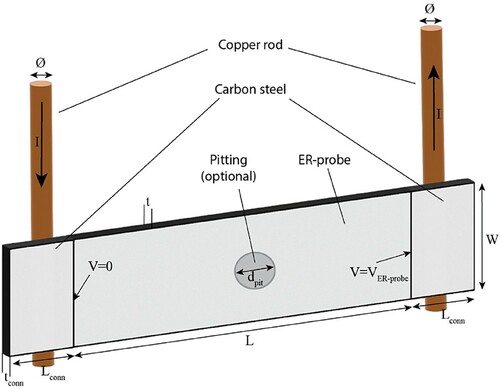
The sandblasted CS was a sheet with a dimension of 60 × 5 × 0.5 mm³. The samples were located in a 3D-printed holder made of acrylonitrile butadiene styrene and sealed from the rear side with a bicomponent acrylic resin. The sample holder allowed the placement of five electrical connections by means of copper rods (diameter of 1.9 mm) from the backside and guaranteed exclusively 1 cm² of exposed steel surface at the front side. The electrical connections were achieved by mechanically pressing the copper rods against the backside of the steel sheet. This allowed avoiding soldering or welding points to the steel, which would have been associated with less well-defined contact points. When rods are soldered to the steel, the contact area will vary between soldered points depending on the amount of the flux used as support material. As a consequence, the exact distance between two measuring points on the same ER-probe might be difficult to estimate. By welding instead, the location of the connection can be better controlled than the soldering approach, but the elevated temperature required for the welding may thermally affect the steel, potentially affecting its corrosion behaviour. Using the designed sample holder, it was possible to guarantee precision in the location of the copper rod (in the order of 0.1 mm) without compromising the corrosion behaviour of the steel, avoiding elevated temperatures. With the geometry designed for the sample holder, when the sample was exposed to a corrosive environment, only one dimension (thickness) was subjected to modification. Figure 1 shows the front side, the rear side and the schematic representation of the used ER-probe.

Figure 1. Photo of the front side (a), rear side (b) and schematic representation of the ER-probe (c) used in this study. Here I represents the applied current, V_Sample and V_Reference represent the measured voltage of the exposed sample and the isolated part, respectively.

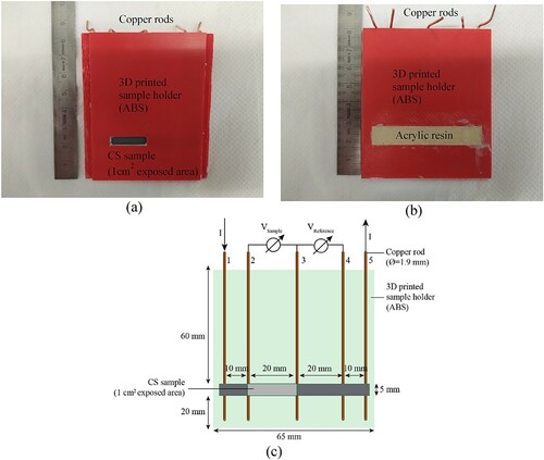
The copper rods allowed the application of the current, I, between the connection 1 and 5 and the voltage measurements between the points 2 and 3, and 3 and 4. The current (0.5 A) was applied by a Solartron-Schlumberger 1286, while the voltage measurements were performed by using a Keithley 2701.

The presence of a second reference element made of the same material, with identical geometry and completely isolated from the testing solution was allowed to exclude other parameters (i.e. temperature) which would interfere in the data evaluation. To remove possible contributions of temperature fluctuations during the experiments, the voltage values measured for the exposed sample, V_Sample, were normalised with the values of voltage measured for the embedded part, V_Reference.

The normalised voltages (V_Norm), equal to the ratio between V_Sample and V_Reference, were converted to thickness with Equation (1). (1) $t\left(\tau \right)={\displaystyle \frac{{\rho }_{\mathrm{S}\mathrm{a}\mathrm{m}\mathrm{p}\mathrm{l}\mathrm{e}}}{{\rho }_{\mathrm{R}\mathrm{e}\mathrm{f}\mathrm{e}\mathrm{r}\mathrm{e}\mathrm{n}\mathrm{c}\mathrm{e}}}\cdot {\displaystyle \frac{t_0}{V_{\mathrm{N}\mathrm{o}\mathrm{r}\mathrm{m}}\left(\tau \right)}}}$(1) where $t$ is the thickness of the sample in µm, $\tau$ represents the time, $t_0$ is the initial thickness (here equal to 500 µm), ${\rho }_{\mathrm{S}\mathrm{a}\mathrm{m}\mathrm{p}\mathrm{l}\mathrm{e}}$ represents the resistivity of the sample in Ω m, ${\rho }_{\mathrm{R}\mathrm{e}\mathrm{f}\mathrm{e}\mathrm{r}\mathrm{e}\mathrm{n}\mathrm{c}\mathrm{e}}$ represents the resistivity of the reference element in Ω m and $V_{\mathrm{N}\mathrm{o}\mathrm{r}\mathrm{m}}$ represents the normalised voltage as a function of time. When assuming identical temperature and identical resistivity of sample and reference element, the ratio ${\rho }_{\mathrm{S}\mathrm{a}\mathrm{m}\mathrm{p}\mathrm{l}\mathrm{e}}$/${\rho }_{\mathrm{R}\mathrm{e}\mathrm{f}\mathrm{e}\mathrm{r}\mathrm{e}\mathrm{n}\mathrm{c}\mathrm{e}}$ is equal to 1.

The experimental time for these measurements was 14 days and for each of the studied solutions, three samples were studied.

Electrochemical measurements

LPR and EIS measurements were performed with Metrohm Autolab PGSTAT302N. Figure 2 shows a schematic representation of the standard three-electrode setup used in this study.

Figure 2. Schematic representation of the three-electrode setup used for electrochemical measurements.

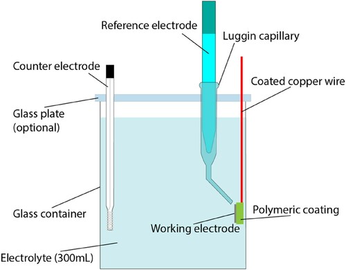
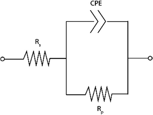
The working electrode was a sandblasted CS sample of thickness approx. 500 µm soldered to copper wire to ensure electric connection and embedded in bicomponent acrylic resin with an exposed surface of 1 cm². The reference electrode was Ag/AgCl sat. KCl and a platinum wire was used as a counter electrode. For the experiment with reduced oxygen concentration, a glass plate was used to cover the glass container in order to limit the diffusion of oxygen from the atmosphere to the working solution. LPR measurements were performed from –15 to +15 mV, with respect to open circuit potential at a scan rate of 10 mV min⁻¹. The Ohmic drop (IR) corrections on the LPR data were performed a posteriori using the solution resistance obtained from the EIS measurements. The IR-corrected LPR data were linearly fitted to extrapolate the polarisation resistance (R_p). The Root-Mean-Square (RMS) amplitude of the applied sinusoidal AC voltage for the EIS measurements was 15 mV in all the experiments. The spectra of frequencies were recorded in the range from 50 000 to 0.01 Hz. The EIS measurements were analysed with the equivalent circuit represented in Figure 3. To perform the fitting of the experimental data and the simulation of the equivalent circuit, the open-source platform, pyEIS, was used [31].

Figure 3. Equivalent circuit used to fit the EIS data. R_s represents the solution resistance, CPE is a constant phase element and R_p is the polarisation resistance.

The R_p normalised to the exposed area of the sample (1 cm²) was used to calculate the CR by means of the Stern–Geary equation [9]. For this calculation, a Stern–Geary coefficient of 26 mV [32] was used for all the conditions, and a conversion factor of 11.6 was used to convert from current density (µA cm⁻²) to sectional loss µm y⁻¹. The experimental time for these measurements was 14 days, as this was sufficient to lead to appreciable results in all cases. The measurements were performed once per day in the case of the condition with reduced oxygen. Whereas, in the remaining conditions, the measurements were performed between days 0 and 7 and 11 and 14. For each of the studied solutions, three replicate samples were considered.

Weight loss measurements

For the weight loss measurements, seven replicate samples (exposed surface: 2 cm²) were immersed in solution by means of nylon wires (Figure 4). Deionised water was added to maintain the volume of the solution constant over the testing period. The lid of the desiccator was used only for the condition of reduced oxygen content; for all the other experiments, the container was left uncovered.

Figure 4. Schematic representation of the setup used for the weight loss measurements.

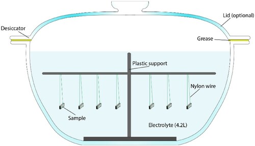
After the corrosion test in the exposure solution, the corroded samples were cleaned to remove oxide scales. For this purpose, the samples were immersed in 37% HCl solution for less than 30 s, followed by rinsing in ultrapure water and ethanol. This cleaning procedure was tested on freshly prepared samples to quantify the loss of material related to this process. Seven samples were tested, with the result of an average loss of material of 0.43 ± 0.45 mg with a maximum loss of 1.0 mg. Accordingly, the experimental time of the weight loss experiments was planned to have a weight loss significantly greater than the error related to this cleaning procedure. The maximum error of 1 mg due to the cleaning procedure was used to correct the weight loss values obtained in the experiments.

The experimental time varied depending on the studied solution, as summarised in Table 2. For the alkaline solution, the samples were immersed for 7 days in the solution at pH approx. 13. After that, 73.63 g of NaCl was added (to yield chloride concentration 0.3 M), and the samples remained in this environment for further 42 days.

Table 2. Experimental time in days for the weight loss measurement in the different environmental conditions considered.

Experimental condition	Experimental time [d]
Alkaline solution	49 (7 chloride-free + 42 after NaCl addition)
Simulated soil	41
Artificial seawater	41
Reduced oxygen content	22

Numerical model

A finite element model of ER-probes was performed by using Comsol Multiphysics®. The model was based on Ohm’s law (Equation (2)): (2) $\overrightarrow{J}=\sigma \cdot \overrightarrow{E}$(2) where $\overrightarrow{J}$ is the current density in A/m², $\sigma$ is the conductivity in S/m and $\overrightarrow{E}$ is the electric field in V/m. The geometry of the sample considered in the model is represented schematically in Figure 5.

Figure 5. Schematic representation of the geometry used in the finite element model.

The geometry of the model was selected to replicate the ER-probe geometry of the experiments. Thermal effects were not considered, and therefore the second steel element (reference) used in the experiments was not included in the model. The voltage was taken at one of the extremities of the sample (V), while on the other extremity, the voltage was set to zero as initial condition. Table 3 summarises the parameters used in the model.

Table 3. Geometrical and input parameters used in the finite element model.

Parameter	Value	Unit	Description
I	0.5	A	External current applied
L	20	Mm	Length of the ER-probe
W	5	Mm	Width of the ER-probe and the steel connection
t0	0.5	Mm	Initial thickness of the sample
t	0 < t < 0.5	Mm	Thickness of the sample, variable for uniform corrosion study
tconn	0.5	mm	Thickness of the steel connection
Lconn	5	mm	Length of the steel connection
Ø	1.9	mm	Diameter of the copper rods
dpit	0–4.99	mm	Pit diameter, variable in the study on localised corrosion
tpit	0–0.5	mm	Depth of the pit, variable in the study on localised corrosion
${\sigma }_{\mathrm{s}\mathrm{t}\mathrm{e}\mathrm{e}\mathrm{l}}$	10^7	S m^−1	Conductivity of steel
${\sigma }_{\mathrm{c}\mathrm{o}\mathrm{p}\mathrm{p}\mathrm{e}\mathrm{r}}$	10^10	S m^−1	Conductivity of copper
V0	0.4	mV	Voltage across the ER-probe during the application of current, I, in pristine state. (Calculated with Equation (3))
VER-probe	Calculated	mV	Voltage across the corroded ER-probe (modelled)
ΔVER-probe	Calculated	mV	VER-probe − V0
δ	7.87	g cm^−3	Density of carbon steel

With the geometry considered and current applied, it is possible to calculate the voltage across the ER-probe in the pristine state (V₀) by means of Pouillet’s law (Equation (3)): (3) $V_0=I\cdot {\displaystyle \frac{1}{{\sigma }_{\mathrm{s}\mathrm{t}\mathrm{e}\mathrm{e}\mathrm{l}}}\cdot {\displaystyle \frac{L}{W\cdot t_0}}}$(3) Here, $I$ is the applied current in Ampere, ${\sigma }_{\mathrm{s}\mathrm{t}\mathrm{e}\mathrm{e}\mathrm{l}}$ is the conductivity of the carbon steel in S/m, and L, W and t₀ correspond to length, width and initial thickness of the ER-probe in metres, respectively, as reported in Table 3.

Here, the value of V₀ is 0.4 mV. V_ER-probe was obtained from the finite element model for different geometrical variations representing different corrosion situations. Subsequently, ΔV_ER-probe was calculated as the difference of V_ER-probe and V₀ (Table 3).

Two corrosion mechanisms were investigated: uniform corrosion and localised corrosion. For the first, the thickness of the sample (t) was reduced from 500 to 1 µm in steps of 1 µm.

For the second, pits with cylindrical shapes were considered. On the one hand, the pit diameter was fixed to 200 µm the and the depth of the pit varied until perforation of the steel occurred. On the other hand, by fixing the pit depth (t_pit), the diameter of the pit (d_pit) varied between 2 µm and 4.99 mm with steps of 1 µm.

Joule effect

The passage of electrical current through a resistor dissipates energy and leads to heating of the resistor. This is known as the Joule effect. The energy dissipated due to the application of a current is I²·R·τ. The definition of heat is m·C_p·ΔT, where m is the mass and C_p is the specific heat capacity and ΔT is the temperature change [33]. Combining these expressions with the Pouillet’s Law, the temperature change generated in the metal was calculated with Equation (4). (4) $\mathrm{\Delta }T=I^2\cdot \rho \cdot {\displaystyle \frac{\tau }{W^2\cdot t^2\cdot C_p\cdot \delta }}$(4) where ΔT is the heat generated in degree Celsius (°C), I is the applied current in Ampere, $\rho$ is the resistivity in Ω·m, δ is the density of steel in kg/m³, W is the width of the ER-probe as shown in Table 3, t is the variable thickness in metres of the ER-probe as shown in Table 3, $\tau$ is the time in seconds of the applied current, and $C_p$ is the specific heat capacity of iron equal to 452 J kg⁻¹ °C⁻¹ [34]. For this calculation, it is assumed that the time of current application necessary for the voltage measurements was 10 s.

Effects of thermal losses of the probe during the measurements, e.g. due to radiation and thermal conductance (e.g. contact with electrolyte), are neglected in this model, which leads to conservative calculations.

Results

Thickness vs. time

With the use of ER-probes, it was possible to monitor the variation of the thickness of the sample over the experimental time. The data were linearly fitted, and the slope corresponds to the CR and the intercept corresponds to the initial thickness (t₀) of the sample. These values are reported in the legend of the figures showing the ER-probes data. Figure 6 shows representative examples of the ER-probes immersed in the four different solutions.

Figure 6. Example of ER-probe data for (a) alkaline solution, the dashed line correspond to the time at which NaCl was added to the solution. The two continous lines correspond to the linear regression of the data points before and after additon of NaCl; (b) artificial seawater; (c) simulated soil and (d) reduced oxygen content solution. In the legend, for each example, the slope in the form of CR expressed in µm y⁻¹ and the intercept of the linear regression, which correspond to the initial thickness (t₀).

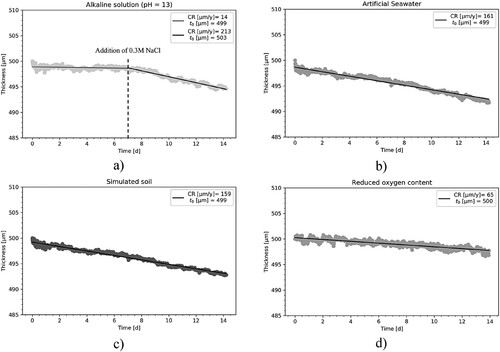
In Figure 6(a), the value of the thickness measured with ER-probes prior to the addition of NaCl remained between 500 and 498 µm, corresponding to an average CR of 14 µm y⁻¹ over the experimental time. From day 7 (when the NaCl was added), the slope showed a significant change, and the measured thickness decreased by about 5 µm in the remaining 7 days, with an average CR of 213 µm y⁻¹ over the last 7 days. Similarly, the average CRs over the experimental time were 161 µm y⁻¹ in artificial seawater, 159 µm y⁻¹ in simulated soil, and 65 µm y⁻¹ in the reduced oxygen content solution.

CR vs. time

Figure 7 shows the CR determined with the different techniques and in the different electrolytes. With the use of LPR and EIS measurements, it was possible to monitor the instantaneous CR. Weight loss measurements and ER-probe showed an average CR over the experimental time.

Figure 7. CR in (a) alkaline solution evaluated with weight loss, ER-probe, EIS, LPR before and after addition of NaCl, (b) artificial seawater, (c) simulated soil solution and (d) reduced oxygen content solution. For the weight loss measurement and the ER-probe, an average CR over the experimental time is represented by the continous line, while the shade represent the standard deviation calculated on seven and three samples, respectively. The blue and dark blue markers represent the average value with standard deviation of the instantaneous CR calculated on three different samples with EIS and LPR, respectively The vertical dashed line located at day 7 corresponds to the time at which NaCl was added to the alkaline solution.

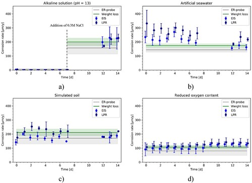
In the alkaline electrolyte, the simulated soil and the reduced oxygen content solution (Figure 7(a,c,d)), the average CR over the experimental time measured with ER-probes, and the average values of the instantaneous CRs obtained with LPR and EIS generally agree well and did not vary much over time. In artificial seawater (Figure 7(b)), both electrochemical techniques show a decrease in instantaneous CR from 350 µm y⁻¹–150 µm y⁻¹ over the experimental time. This behaviour could not be captured with ER-probes and weight loss measurements.

CR between the different techniques

Figure 8 compares the instantaneous CRs calculated with EIS and LPR, independently from the measurement solution and measurement time.

Figure 8. CR comparison between the electrochemical techniques. The comparison includes all the data recorded in this study. The orange area corresponds to the deviation with factor lower than 2.

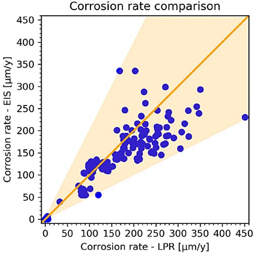
The CR measured with the two techniques showed comparable results, with a difference between the two techniques limited within a factor of 2 in the entire range of CRs considered. As shown in Figure 7(b), for the samples exposed to simulated seawater, over the entire 14 days, the average values of the instantaneous CRs recorded with LPR showed higher values than the average values recorded with EIS. For the samples exposed to simulated soil solution (Figure 7(c)) over the entire 14 days the average values of the instantaneous CRs recorded with LPR showed higher values than the average values recorded with EIS. In the data presented in Figure 7(d), the average values of the instantaneous CRs measured with LPR showed higher values than the ones calculated with EIS. Generally, however, all the data points are in the orange region, which defines the area with a deviation with a factor lower than 2.

To compare the instantaneous CRs calculated with electrochemical techniques with the one obtained with ER-probes and weight loss, the average over the experimental time for LPR and EIS were calculated including all the instantaneous measurements performed (Figure 9).

Figure 9. Average CR and standard deviation over the experimental time for the ER-probes, LPR and EIS in (a) alkaline environment before addition of NaCl, (b) alkaline environment after addition of NaCl, (c) artificial seawater, (d) simulated soil solution and (e) reduced oxygen content solution.

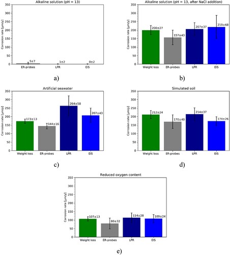
For the passive steel (Figure 9(a)), the ER-probes resulted in a slightly higher CRs than the electrochemical techniques. After the addition of NaCl (Figure 9(b)), the behaviour was the opposite. For CR in the order of 200 µm y⁻¹, the average value calculated with ER-probes is between 21.5% and 28.3% lower than the values obtained with all the other techniques.

In Figure 9(c), the CR calculated with weight loss, ER-probes, LPR, and EIS showed average CRs between 264 and 144 µm y⁻¹. LPR and EIS show an average CR that is 53% and 20% higher than to the value obtained with weight loss, respectively. ER-probes instead showed CR 17% lower than the value obtained with weight loss method, 45% lower than the value obtained with LPR, and 30% lower than the value calculated with EIS.

Similarly, in Figure 9(d), the average CRs over the experimental time in simulated soil solution measured with weight loss, ER-probes, LPR, and EIS were between 170 and 214 µm y⁻¹. The CR measured with LPR and EIS were 1% higher and 18% lower than the measured value with weight loss, respectively. ER-probes showed the lowest CR being 20% lower than the value obtained with weight loss, 21% lower than the value obtained with LPR, and 2% lower than the value obtained with EIS.

Lastly, in Figure 9(e), the CRs in reduced oxygen content solution measured with weight loss, ER-probes, LPR, and EIS were between 80 and 114 µm y⁻¹. The CR measured with LPR and EIS were 7% and 2% higher than the value from weight loss, respectively. ER-probes showed the lowest CR being 25% lower than the value obtained with weight loss, 30% lower than the value obtained with LPR, and 26% lower than the value obtained with EIS.

Numerical models

Uniform corrosion

Figure 10 shows the modelled change in voltage across the ER-probe (ΔV_ER-probe) as a function of the thickness (t) and the initial thickness (t₀). For this model, the thickness of the sample was varied from 500 to 5 µm (t/t₀ equal to 1 and 0.01, respectively).

Figure 10. Modelled ER-probe behaviour for uniform corrosion: measurable voltage change, ΔV_ER-probe, as a function of the ratio between the variable thickness of the ER-probe (t) and the ER-probe in the pristine state (t₀).

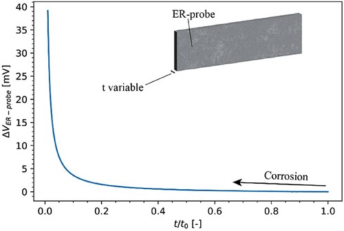
The decrease in t/t₀ resulted in an increase of the ΔV_ER-probe measured. In agreement with Equation (3), there is an inverse relationship between the voltage and t/t₀, with a steep increase in ΔV_ER-probe for t/t₀ approaching 0.01. The ΔV_ER-probe in the region of t/t₀ between 1.0 and 0.2 showed minor voltage changes lower than 2 mV.

Localised corrosion

In the first localised corrosion model, three different d_pit/W were considered, and the depth of the pit (t_pit) was varied until reaching the perforation of the probe (t_pit/t = 1). Figure 11 shows ΔV_ER-probe as a function of the ratio between the pit depth and the thickness of the ER-probe.

Figure 11. Modelled ER-probe behaviour for localised corrosion with pits growing in the depth: ΔV_ER-probe as a function of the ratio between the pit depth (t_pit) and the ER-probe thickness (t), considering three different ratios d_pit/W.

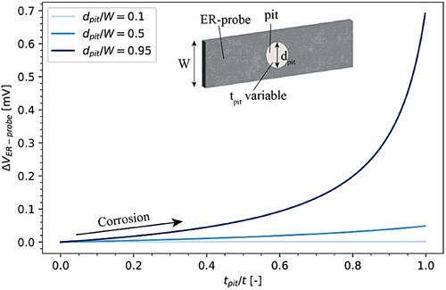
For a small pit with respect to the ER-probe (d_pit/W equal to 0.1), ΔV_ER-probe remained below 1 µV. For d_pit/W equal to 0.5, ΔV_ER-probe increased up to 0.05 mV once the pit penetrated the entire probe. For a large pit (d_pit/W equal to 0.95), ΔV_ER-probe increased exponentially, reaching a maximum of 0.7 mV for t_pit/t equal to 1. However, the effect of the pit depth is significant. If the pit penetrates the probe only by 50%, the observable voltage is lower than 0.1 mV.

In the second case, the influence of lateral pit growth was studied for three t_pit/t (Figure 12). The diameter of the pit (d_pit) was varied up to 4.99 mm (d_pit/W = 0.99).

Figure 12. Modelled ER-probe behaviour for localised corrosion with a pit growing laterally: ΔV_ER-probe in the presence of a pit with three different pit depths (t_pit) and variable pit diameter (d_pit).

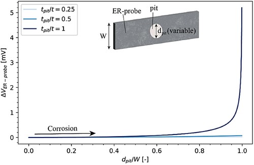
Figure 12 again shows the dramatic influence of the pit depth. Only for pits penetrating the probe thickness, t_pit/t equal to 1, was the probe voltage appreciable. ΔV_ER-probe increased exponentially with increasing d_pit/W. A significant increase in ΔV_ER-probe was found with d_pit/W greater than 0.8, otherwise the maximum observable ΔV_ER-probe was about 0.2 mV. For shallower pits (t_pit/t equal to 0.5 and 0.25), this was even more pronounced and the ΔV_ER-probe, even for d_pit/W equal to 0.99, did not show a significant increase.

In the third case (Figure 13), the influence on ΔV_ER-probe of the number of randomly generated non-overlapping pits was studied. Here, the ratio between the diameter of each pit and the width of the ER-probe was equal to 0.08 and t_pit/t was fixed to 1. Figure 13(b) shows ΔV_ER-probe as a function of the number of pits for different d_pit/W. Three independent calculations were performed to consider a possible stochastic effect of the pit distribution in the ER-probe. However, as is apparent from Figure 13, the stochastic influence was generally negligible.

Figure 13. (a) Modelled ER-probe behaviour for localised corrosion with increasing number of small pits: ΔV_ER-probe as a function of the number of pits with pit depth (t_pit) equal to the ER-probe thickness (t) and diameter equal to 0.08 times the width of the ER-probe. (b) ΔV_ER-probe as a function of the number of pits with complete perforation of the ER-probe, for the difference ratio between the pit diameter (d_pit) and the width of the ER-probe. The horizontal line corresponds to a ΔV_ER-probe of 10 µV. The lines correspond to the mean value of ΔV_ER-probe, while the blue shade corresponds to the standard deviation considering three calculations.

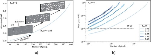
Figure 13 shows that ΔV_ER-probe increased with an increasing number of pits. For d_pit/W equal to 0.08, despite the elevated number of pits, however, ΔV_ER-probe was in the order of a fraction of a millivolt. Indeed, with the presence of 395 distinct pits with complete perforation of the ER-probe (t_pit/t equal to 1) and covering 50% of the probe surface area, ΔV_ER-probe showed a maximum about 1 mV. By considering a constant number of pits, ΔV_ER-probe increased with increasing d_pit/W.

Joule effect

In reality, ER-probes are subjected to different temperatures, e.g. due to daily and seasonal variations. Thus, temperature corrections are needed. A common approach is to combine the exposed ER-probe with a reference element of identical material and dimensions, which, however, is shielded from the corrosive environment, e.g. by a coating. This approach is similar to what was used in this study (Figure 1). Assuming that the reference element has the same temperature as the ER-probe, one can correct for temperature variations without the need for measuring the temperature and applying mathematical temperature corrosions. In such arrangements, the ER probe thickness decreases over time due to corrosion, but the thickness of the reference element remains unchanged. As was discussed in the section “Joule effect”, the passage of the electrical current during the measurement can lead to Joule heating of both elements. When the ER-probe and the reference element have different thickness, e.g. due to corrosion of the ER-probe, the Joule heating may lead to differences in temperature between these two elements and thus potentially lead to a measurement error. Figure 14 shows the temperature difference between the ER-probe (T_ER-probe) and the reference element (T_Reference) as a function of the applied current and t/t₀, calculated with Equation (4).

Figure 14. Temperature difference between the ER-probe and the reference element as a function of t/t₀ and of the applied current, considering a current application of 10 s for the voltage measurement across the ER-probe and the reference. For this simulation, the width and the length for both ER-probe and the reference were 5 and 20 mm, respectively. The thickness of the reference element was equal to t₀ (500 µm), and the thickness, t, of the ER-probe varied between 500 and 0 µm.

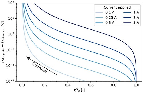
The temperature difference between ER probe and reference element increases with decreasing the ER-probe thickness and with increasing applied current. These temperature effects are generally small, unless t assumes very low values. For t/t₀ < 0.1 and I > 1A, the temperature difference can rise above 10°C.

Discussion

Comparison of measurement methods

CRs from less than 10 to 300 µm y⁻¹ were covered in the experiments. LPR and EIS measurements were able to capture instantaneous CRs, with the deviation between the two techniques lower than factor 2 for the entire range of CRs. ER-probes and weight loss measurements averaged CRs over larger time spans than the electrochemical techniques. ER-probes showed good agreement with the weight-loss method, with a slight tendency to underestimate the CR (with a difference of 17–30%). Similar results were obtained by Liu et al. [30] in 3.5% NaCl with 1 wt-% of silica sand to simulate erosion corrosion, although the order of magnitude of CRs studied by Liu et al. was clearly higher than in this study.

Overall, the average CR measured with ER-probe, weight loss, LPR end EIS over the experimental times showed good agreement between all the techniques in the different environments studied (Figure 9). The difference between CR measured with ER-probe and the other techniques was always below 45%.

Type of corrosion mechanism

Passive steel

Steel in alkaline solution with pH 13 (in the absence of chlorides) is known to form a passive layer [35], and the CR is expected to be in the order of 1–10 µm y⁻¹, thus negligibly low [2]. As reported in Figures 6, 7 and 9, ER-probes, LPR and EIS showed a good agreement in the evaluated CRs in the order of 10 µm y⁻¹ or less.

Localised corrosion

After a week of exposure in an alkaline environment, NaCl was added to provoke a localised attack (pitting) on the already formed passive layer of the samples. Figure 15 shows three examples of optical micrographs of samples exposed to an alkaline solution with the addition of 0.3M NaCl.

Figure 15. Optical micrographs of the three samples that were exposed to alkaline solution with addition 0.3M NaCl.

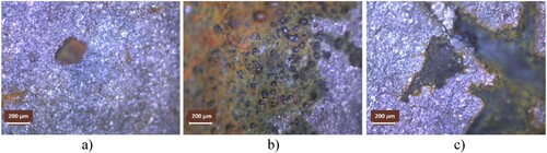
The examples represented in Figure 15 confirmed the localised nature of the corrosion attack induced by the presence of chloride ions in the alkaline solution.

Figure 6 shows a change in calculated thickness after the NaCl addition (day 7). This means that the ER-probe allowed to determine corrosion initiation and subsequently to monitor the corrosion process in situ.

It should be noted that the theory underlying the ER probe technique relies on the assumption of uniform corrosion [10]. However, here we had localised corrosion. Thus, the calculated loss in thickness after corrosion initiation is not reliable and tends to underestimate the attack depth in localised corrosion. The same limitation applies to weight loss measurements and to electrochemical techniques based on polarisation resistance [1–3,5–9]. In this work, the CR evaluated with ER-probes were in the same order magnitude as the ones measured with weight loss and electrochemical techniques.

Uniform corrosion

CS samples exposed to artificial seawater and simulated soil solution with pH ∼7 showed active behaviour, as expected from the Pourbaix diagram [35]. In these environmental conditions, the samples showed corrosion of uniform type with corrosion products covering the entire exposed surface. The CR determined with ER-probes and the weight loss method differed by a maximum of 20% (Figure 9(c,d)).

The difference in average CR over the experimental time measured between the electrochemical techniques and the weight loss can be due the different experimental time between the methods and due to the precipitated layer at the steel surface. These two factors are evident in the case of the instantaneous CR measured with LPR and EIS in simulated seawater (Figure 7(b)). Here, the average values of the instantaneous CR measured with both the techniques have the tendency to decrease over time. The reduction over time in the instantaneous CR is related to an increase in the measured polarisation resistance, which can be attributed to the presence of a precipitated product on the sample surface [36]. Thus, if LPR and EIS had been measured for an experimental time comparable to one of the weight loss methods, the difference between the methods may be smaller.

The difference in experimental time between the ER-probes and the weight loss, instead, should not be considered an influencing factor for the difference in the CR measured. The decrease in thickness recorded by the ER-probes behaved linearly over the studied experimental time, which can be converted in a constant CR over the experimental time. Therefore, it is expected that if the experimental time for the ER-probes would have been in the same range as the one for the weight loss method, unless other corrosion mechanisms take place or corrosion stops, the results obtained with ER-probe would not be different from weight loss method.

Differential aeration (galvanic element)

CS exposed to a solution with reduced oxygen content showed CR in the order of 100 µm y⁻¹ with all the four techniques used. The covered setup allowed to limit the diffusion of oxygen from the atmosphere to the testing solution. The limited presence of oxygen reduced the CR compared to other environmental conditions considered in this study.

However, the different oxygen concentrations at the sample surface promoted the formation of a galvanic element within the samples. Figure 16 shows examples of three samples used to measure CR with electrochemical techniques (Figure 16(a)), with ER-probes (Figure 16(b)) and with weight loss method (Figure 16(c)) exposed to reduced oxygen concentration solution. Here it appears evident that in all the three cases, a part of the sample behaved as an anode, represented by the area covered by corrosion products, and the remaining part of the samples behaved as a cathode, represented by the area where the steel remained clean from corrosion products.

Figure 16. Photo of samples used for measuring CR with electrochemical techniques (a), with ER-probes (b) and weight loss (c) exposed to reduced oxygen concentration solution. The photos were acquired immediately after the extraction of the samples from the testing electrolyte.

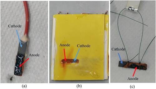
Also, in this non-uniform corrosion case, the average CR over the experimental time measured with ER-probes was in the same range as the one measured with the other techniques (Figure 9(e)). As mentioned in the section “Localised corrosion”, the CR measured with all the techniques relies on the assumption of uniform corrosion; therefore, the calculated loss in thickness might underestimate the actual CR of the carbon steel in these experiments.

ER-probe geometry

With the results obtained with numerical simulations (Figures 10–13), it is possible to optimise the design of ER-probes, depending on the expected type of corrosion. For these studies, a resolution of 10 µV for the voltmeter was conservatively assumed, and the applied current was set to 0.5 A. This assumed resolution of the voltmeter of 10 µV is one order of magnitude higher than the specified resolution of the benchtop multimeter (Keithley 2701) used for the experimental study. The assumption of 10 µV resolution was made to ensure results significantly away from the measurement error of the device and to account for voltmeters with comparable or potentially worse resolution than the benchtop multimeter used in this study. A similar approach was chosen for the simulation of the weight loss measurements. Here, the resolution of the scale was assumed to be 1 mg, which is one order of magnitude higher than the specified resolution of the scale used for the experiments. For both ER-probes and weight loss simulations, it was assumed that the samples are exposed to corrosion only on one side.

Uniform corrosion

For the simulation performed to detect uniform corrosion with ER-probes, a measurement time of one week was considered at CRs of 50, 100, 200, 500 and 1000 µm y⁻¹. The essential question was to study if ER-probes are suitable to detect the metal loss occurring within a week at these different CRs, depending on the ER-probe dimensions. The width of the ER-probe (W) was maintained between 1 and 10 mm, while the length of the ER-probe (L) varied from 1 to 100 mm (Figure 5). Figure 17(a) shows the relationship between minimum width and a maximum length of the ER-probe needed to detect different CRs within a week. The lines correspond to a ΔV_ER-probe, equal to 10 µV, that is, the assumed resolution of the voltmeter. Figure 17(b) shows the relationship between the minimum width and a minimum length of a steel sample in order to detect CRs of 50, 100, 200, 500 and 1000 µm y⁻¹ within a week by means of weight loss method. The lines correspond to a weight loss of 1 mg, that is, the assumed resolution of the scale.

Figure 17. (a) Relationship between maximum width and minimum length of a CS ER-probe to allow detecting the CR indicated in the lines within a week. For this purpose, the lines correspond to a ΔV_ER-probe, equal to 10 µV, assuming an initial thickness of the ER-probe (t₀) of 500 µm, and applied current of 0.5 A. (b) Relationship between the minimum width and minimum length of a carbon steel sample necessary to detect the CR indicated in the lines in a week. For this purpose, the lines correspond to a weight loss of 1 mg. The arrows in figures (a) and (b) indicate the domain in which corrosion detection for the specified case is possible.

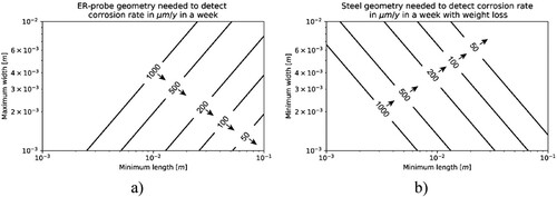
To detect CRs in the order of 50 µm y⁻¹ after one week, with assumptions made in these simulations, the design of the ER probe should have a length between 50 and 100 mm and a width between 1 and 2 mm, respectively. With increasing CRs, the geometrical constraints are not as critical as in the case with 50 µm y⁻¹, as expected by solving Equation (3). The results of the experimental studies (Figures 6, 7 and 9) confirmed the sensitivity of the ER-probes for the CR considered in the simulation. For the experiments with passive steel, the experiments were more sensitive than the simulations, detecting CR in the order of 10 µm y⁻¹. This can be explained by the multimeter resolution, which was10 times higher than the one considered for the simulations.

Nevertheless, Figure 17(a) highlights that the width and length, especially their ratio, are important for the design of ER-probes. The longer the ER-probe, the wider it can be without compromising its sensitivity. For weight loss measurements, the ratio of width and length is not important. It is rather the exposed surface area that matters. Figure 18 shows the overlap of the results shown in Figure 17(a,b) for CR of 200 µm y⁻¹. The dashed line corresponds to the result from weight loss, and the solid line corresponds to the result obtained with ER-probes.

Figure 18. Overlap ER-probes and weight loss geometry constraint for the detection of CR of 200 μm y⁻¹ within one week.

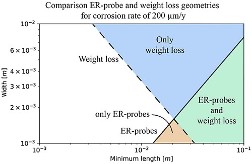
In Figure 18, depending on the ER-probe and sample dimensions, four distinct areas can be identified: the white area corresponds to the geometry combinations where neither ER-probe nor weight loss method can detect a CR of 200 µm y⁻¹ within one week; the orange area (namely ‘only ER-probes’ region) corresponds to a combination of width and length of the sample where only ER-probe could detect such a CR; the light blue area (namely ‘only weight loss’ region) represents a combination of width and length where only weight loss method may be able to detect such a CR; and the green area (namely ‘ER-probes and weight loss’ region) is where geometrical conditions satisfy requirements for both ER-probe and weight loss to detect CR of 200 µm y⁻¹ within one week. In summary, weight loss and ER-probes show comparable sensitivity, with ER-probes slightly more sensitive than weight loss.

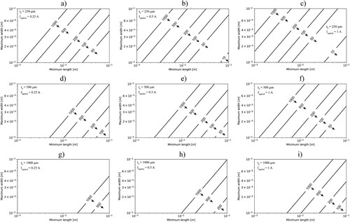
The resolution of the ER probes can be optimised not only by geometrical modifications but also by increasing the applied current for the measurements. In this regard, calculations neglecting the Joule effect were performed for the initial thickness of 250, 500 and 1000 µm, and applied current of 0.25, 0.5 and 1 A.

Figure 19 shows that increasing the applied current improves the resolution of the ER-probe. According to Equation (3), the sensitivity of the ER-probe increases linearly with the applied current. However, as apparent from Equation (4), the increase in temperature of the ER-probe depends on I². Thus, the benefit in terms of probe sensitivity from increasing the applied current is comparatively moderate with respect to potential effects related to Joule heating. With an ER-probe similar to the one used in this work (W = 5 mm, L = 20 mm, t₀ = 0.5 mm), a temperature increase >10°C is expected as soon as t/t₀<0.1 for I > 1A (Figure 14). The electrical resistivity of steel changes by about 0.5% per °C[37]. Thus, 10°C would be ∼5% in terms of measurement error. According to Equation (1), an error in resistivity directly translates into error in thickness and thus CR. In the light of the experimental findings of this study, namely, the comparison of ER-probes with LPR, EIS and weight loss measurements, it appears that such an error related to Joule heating is acceptable. However, as shown in Figure 14, when t decreases further, Joule heating increases non-linearly. Thus, for small residual probe thickness, Joule heating may become an important error source. Figure 14 shows that this can effectively be avoided by keeping I small.

Figure 19. Relationship between maximum width and minimum length of a CS ER-probe to allow detecting the CR indicated in the lines within a week. For this purpose, the lines correspond to a ΔV_ER-probe, equal to 10 µV, assuming an initial thickness of the ER-probe (t₀) of 250, 500 and 1000 µm (increasing vertically), and applied current (I_applied) of 0.25, 0.5 and 1 A (increasing horizontally) as shown in the legend of each figure.

Note that by optimising the measuring equipment and reducing the measurement time, it is possible to reduce the Joule effect further. However, as shown in Equation (4), the Joule effect depends linearly on the measurement time, while the parameters applied current (I), ER-probe width (W) and thickness (t) appear to the power of 2 and are thus predominant in the error development. Note that the length of the ER-probe (L) does not influence the Joule effect. By increasing the length of the ER-probe, it is possible to increase the sensitivity of the ER-probe, as shown in Figures 17 and 19, without introducing further measurements error.

Localised corrosion

As shown in Figure 13(b), the most important parameter for detecting pitting corrosion is the ratio between the diameter of the pit (d_pit) and the width of the ER-probe (W). To detect a single pit with a resolution of the voltmeter of 10 µV, the diameter of the pit shall be ∼0.25 times the width of the ER-probe (Figure 11). However, for d_pit/W equal to 0.08, the presence of at least 10 distinct pits is necessary to be detected (Figure 13(b)). In order to detect localised corrosion with ER-probes, it is important to consider two aspects of the ER-probe geometry. Firstly, the thickness of the ER-probe should be as thin as possible to promote perforation (Figure 12). Secondly, the width of the ER-probe should be as small as possible (Figure 11). Instead, the length of the ER-probe does not play a significant role. However, it should be considered that the pitting resistance increases with decreasing the size of the probe [38–41]. Therefore, reduced size probes might not be representative of the structure that it is monitored.

Implication for engineers

With this study, the reliability of the ER-probes compared to other conventional techniques has been verified. The CRs considered in this study correspond to conditions in which ER-probes may be used in field applications. For example, ER-probes are commonly used buried in soil under a cathodic protection current. In this condition, the environment at the surface of the protected steel becomes alkaline and the oxygen concentration decreases [42–54]. ER-probes may be used to monitor the effectiveness of the cathodic protection system, maintaining the CR of the protected structure to negligible values (<10 µm y⁻¹) or detecting a possible corrosion initiation due to, for example, microbiological activity.

In similar circumstances, ER-probes may be used in reinforced concrete structures in order to monitor the possible corrosion initiation due to carbonation or chloride-induced corrosion. In this case, when the reinforcement is in uncontaminated concrete, it is expected to form a passive layer² which would represent the experimental condition reported in Figure 6 between days 0 and 7. When contamination occurs, either by CO₂ (carbonation) or by chloride ingress (chloride-induced corrosion), the reinforcement may start corroding, representing the experimental situation recreated in Figure 6.

Conclusions

From this experimental and numerical study, the following major conclusions can be drawn:

• ER-probes can determine CRs with comparable accuracy to LPR, EIS and weight loss in both uniform and localised corrosion. The difference between CR measured with ER-probe and the other techniques was always below 45% (in the studied range of CRs from almost 0 to approx. 300 micrometer/year).

• Consideration of the geometrical dimensions is important to optimise ER-probes. Their thickness not only determines the useful life of an ER-probe, but, together with length and width, considerably impacts the sensitivity of the probe. The following recommendations can be made:

  • If uniform corrosion is expected, increasing the length of the probe is the most effective design parameter to improve the sensitivity towards resolving instantaneous CRs down to a few tens of μm y⁻¹ within a period of the order of a week.

  • If pitting corrosion is expected, minimising the width and thickness of the probe are the most effective design parameters to improve the sensitivity for the detection of the onset of pitting corrosion.

  • Design charts such as the ones proposed in this paper can be used in selecting dimensions (width, length and thickness) to optimise the ER-probe with respect to the corrosion regime expected for a certain application.

• Joule heating of the ER-probe may become a source of error in the evaluation of the CR, particularly when the probe becomes very thin. Caution should be exercised when increasing the applied current during the measurement due to the non-linear influence of current on Joule heating.

Acknowledgements

The authors wish to thank Francesco Lovisi for the support given for this study.

Disclosure statement

No potential conflict of interest was reported by the author(s).

Additional information

Funding

The authors are grateful to the European Research Council (ERC) for the financial support provided under the European Union’s Horizon 2020 research and innovation program (grant agreement no. 848794). Additionally, the authors acknowledge the industrial partners Gaznat SA, Gasverbund Mittelland AG, Erdgas Ostschweiz AG and Transitgas AG for their financial support.

References

- Yang L. Techniques for corrosion monitoring. Cambridge: Woodhead Publishing; 2020. 620p.
- Bertolini L, Elsener B, Pedeferri P, et al. Corrosion of steel in concrete: prevention, diagnosis, repair. Weinheim (Germany): Wiley; 2013.
- Pedeferri P, Ormellese M. Corrosion science and engineering. Cham (Switzerland): Springer; 2018.
- McKenzie M, Vassie PR. Use of weight loss coupons and electrical resistance probes in atmospheric corrosion tests. Br Corros J. 1985;20:117–124.
- Lorenz WJ, Mansfeld F. Determination of corrosion rates by electrochemical DC and AC methods. Corros Sci. 1981;21:647–672.
- Andrade C, Alonso C. Corrosion rate monitoring in the laboratory and on-site. Constr Build Mater. 1996;10:315–328.
- Kelly RG, Scully JR, Shoesmith D, et al. Electrochemical techniques in corrosion science and engineering. New York: CRC Press; 2002. 442p.
- Frankel GS. Electrochemical techniques in corrosion: status, limitations, and needs. J ASTM Int. 2008;5:1–27.
- Geary AL. Electrochemical Polarization. J Electrochem Soc. 1957;8.
- Brossia CS. Electrical resistance techniques. In: Techniques for corrosion monitoring. Duxford (UK): Elsevier; 2021. p. 267–284. https://doi.org/https://doi.org/10.1016/B978-0-08-103003-5.00011-4
- Cai J-P, Lyon SB. A mechanistic study of initial atmospheric corrosion kinetics using electrical resistance sensors. Corros Sci. 2005;47:2956–2973.
- Cooper G. In: G Moran, P Labine, editors. Corrosion monitoring in industrial plants using nondestructive testing and electrochemical methods. Sensing Probes and Instruments for Electrochemical and Electrical Resistance Corrosion Monitoring. ASTM International; 1986. p. 237–237–14. http://www.astm.org/doiLink.cgi?STP17449S.
- Li S, Jung S, Park K, et al. Kinetic study on corrosion of steel in soil environments using electrical resistance sensor technique. Mater Chem Phys. 2007;103:9–13.
- Li S, Kim Y-G, Jung S, et al. Application of steel thin film electrical resistance sensor for in situ corrosion monitoring. Sens Actuators B. 2007;120:368–377.
- Li Z, Fu D, Li Y, et al. Application of an electrical resistance sensor-based automated corrosion monitor in the study of atmospheric corrosion. Materials. 2019;12:1065.
- Kouril M, Prosek T, Scheffel B, et al. High sensitivity electrical resistance sensors for indoor corrosion monitoring. Corros Eng Sci Technol. 2013;48:282–287.
- Kouril M, Prosek T, Scheffel B, et al. Corrosion monitoring in archives by the electrical resistance technique. J Cult Herit. 2014;15:99–103.
- Denzine AF, Reading MS. A critical comparison of corrosion monitoring techniques used in industrial applications. Corrosion. 1997;97.
- Shukla PK, DeWitt J, Krissa LJ, et al. Monitoring Effectiveness of Vapor Corrosion Inhibitors for Tank Bottom Corrosion Using Electrical Resistance Probes and Coupons. NACE International Corrosion Conference proceedings; 2019. p. 1–10.
- Whited T, Yu XA, Tems R. Mitigating soil-side corrosion on crude oil tank bottoms using volatile corrosion inhibitors. Corrosion. 2013;2013:1–12. Paper No. 2242.
- Gartner N, Kosec T, Legat A. Monitoring the corrosion of steel in concrete exposed to a marine environment. Materials. 2020;13:407.
- Legat A. Monitoring of steel corrosion in concrete by electrode arrays and electrical resistance probes. Electrochim Acta. 2007;52:7590–7598.
- Jansen S, van Burgel M, Gerritse J, et al. Cathodic protection and MIC-effects of local electrochemistry. CORROSION 2017; 2017.
- Junker A, Møller P, Nielsen LV. Effect of chemical environment and PH on AC corrosion of cathodically protected structures. NACE International Corrosion Conference proceedings. NACE International; 2017. p. 1–14.
- Khan NA. Use of ER soil corrosion probes to determine the effectiveness of cathodic protection. CORROSION 2002, OnePetro; 2002.
- Song H-S, Kho Y-T, Kim Y-G, et al. Competition of AC and DC current in AC corrosion under cathodic protection. CORROSION 2002, OnePetro;2002.
- Gunars Bracs EB, Orchard DF. Use of electrical resistance probes in tracing moisture permeation through concrete. ACI J Proc. 1970;67. https://doi.org/https://doi.org/10.14359/7302.
- Bell GE, Moore CG, Williams S. Development and application of ductile iron pipe electrical resistance probes for monitoring underground external pipeline corrosion. CORROSION 2007, OnePetro; 2007.
- Jarragh A, Al-Sulaiman S, Khuraibut Y, et al. Microbiologically influenced corrosion by general aerobic and anaerobic bacteria in oil & gas separators. CORROSION 2014, OnePetro; 2014.
- Liu L, Xu Y, Xu C, et al. Detecting and monitoring erosion-corrosion using ring pair electrical resistance sensor in conjunction with electrochemical measurements. Wear. 2019;428–429:328–339.
- Knudsen KB. Pyeis: a Python-based electrochemical impedance spectroscopy analyzer and simulator. Electrochem Soc. 2019:1937–1937.
- Buchanan RA, Stansbury EE. Handbook of environmental degradation of materials. Elsevier; 2012. p. 87–125. https://linkinghub.elsevier.com/retrieve/pii/B9781437734553000043.
- Peter Atkins P, De Paula J. Atkins’ physical chemistry. Oxford: OUP; 2014.
- Austin J. Heat capacity of iron – a review. Ind Eng Chem. 1932;24:1225–1235.
- Deltombe E, Pourbaix M. Equilibrium potential-PH diagrams for iron at 25 C. Reun Com Int Thermodyn Dyn Cinet Electrochim. 1955;6:124–157.
- Martinelli-Orlando F, Shi W, Angst U. Corrosion behavior of carbon steel in alkaline, deaerated solutions: influence of carbonate ions. J Electrochem Soc. 2020;167:061503.
- Yafei S, Dongjie N, Jing S. Temperature and carbon content dependence of electrical resistivity of carbon steel. IEEE, 2009; p. 368–372.
- Burstein G, Ilevbare G. The effect of specimen size on the measured pitting potential of stainless steel. Corros Sci. 1996;38:2257–2265.
- Angst U, Rønnquist A, Elsener B, et al. Probabilistic considerations on the effect of specimen size on the critical chloride content in reinforced concrete. Corros Sci. 2011;53:177–187.
- Angst UM, Elsener B. The size effect in corrosion greatly influences the predicted life span of concrete infrastructures. Sci Adv. 2017;3:e1700751.
- Li L, Sagues A. Chloride corrosion threshold of reinforcing steel in alkaline solutions – effect of specimen size. Corrosion. 2004;60:195–202.
- Glass G, Chadwick J. An investigation into the mechanisms of protection afforded by a cathodic current and the implications for advances in the field of cathodic protection. Corros Sci. 1994;36:2193–2209.
- Martinelli-Orlando F, Angst UM. CP of steel in soil: temporospatial PH and oxygen variation as a function of soil porosity. In: Pipeline Integrity; 2021.
- Junker A, Nielsen LV. Effect of chemical environment and PH on AC corrosion of cathodically protected structures. NACE International; 2017.
- Ackland BG, Dylejko KP. Critical questions and answers about cathodic protection. Corros Eng, Sci Technol. 2019;54:688–697.
- Büchler M, Angst U, Ackland B. Cathodic protection criteria: a discussion of their historic evolution. In: 20th International Corrosion Congress & Process Safety Congress (EUROCORR 2017); 2017.
- Angst U, Büchler M, Martin B, et al. Cathodic protection of soil buried steel pipelines – a critical discussion of protection criteria and threshold values. Mater Corros. 2016;67:1135–1142.
- Gan F, Sun Z-W, Sabde G, et al. Cathodic protection to mitigate External corrosion of underground steel pipe beneath disbonded coating. Corrosion. 1994;50:804–816.
- Gummow R, Segall S, Fingas D. An alternative view of the cathodic protection mechanism on buried pipelines. Mater Perform. 2017;56:32–37.
- Martinelli-Orlando F, Angst U. Effect of soil porosity on the near-field PH of buried steel under CP condition. CeoCor 2021; 2021.
- Martinelli-Orlando F, Shi W, Angst U. Investigation of PH and oxygen variations on steel electrode under cathodic protection. CeoCor 2019 International Congress & Technical Exhibition; 2019.
- Attarchi M, Brenna A, Ormellese M. Cathodic protection and DC non-stationary anodic interference. J Nat Gas Sci Eng. 2020;82:103497.
- Attarchi M, Brenna A, Ormellese M. PH measurement during cathodic protection and DC interference. CORROSION 2021; 2021.
- Brenna A, Ormellese M, Lazzari L. Electromechanical breakdown mechanism of passive film in alternating current-related corrosion of carbon steel under cathodic protection condition. Corrosion. 2016;72:1055–1063.