Evolution of triple junctions’ network during severe plastic deformation of copper alloys – a discrete stochastic modelling

ABSTRACT

Proposed is a methodology for an accurate description of triple junctions’ network evolution in the course of severe plastic deformation (SPD). It is based on representations of polycrystalline solids with discrete combinatorial complexes, processes evolving different substructures (grains, grain boundaries, triple junctions) of these complexes, and methods for analyses of such substructures. It is demonstrated that the methodology can reproduce theoretical results available for the simplest case of quasi-homogeneous microstructure evolution, i.e. spatially random conversion of low to high angle grain boundaries during SPD. It is further shown that the proposed discrete approach can reproduce in a natural way results from recent experiments with copper alloys, where inhomogeneity development during SPD is strongly manifested. Finally, the evolution of different types of triple junctions and their connectivity is analysed to show that these substructure characteristics differentiate inhomogeneous from homogeneous evolution of the polycrystalline solid. It is suggested that such substructure characteristics can form the basis for characterisation of continuous dynamic recrystallisation process.

KEYWORDS:

• copper alloys
• defect structures
• severe plastic deformation
• continuous dynamic recrystallization
• grain boundary engineering
• high-angle grain boundaries

1. Introduction

Grain boundary engineering (GBE) is a wide research area [1–3], where progress in experimental materials’ characterisation [4,5], is complemented by modern mathematical tools, such as topology, percolation theory, discrete analysis, etc. [6–9], in order to advance the understanding of structure-properties relations in materials. The principal use of such understanding is in optimising desired material properties by altering the material microstructure, specifically the nature and spatial distribution of grain boundaries. Hence, the focus of GBE research to date has been in developing appropriate processing technologies that provide final microstructures with improved function-specific performance [2]. To a much lesser extent have the GBE techniques been used to study the microstructure evolution during materials’ processing. One familiar example of a process, where grain boundary structure of the material changes dramatically, is severe plastic deformation (SPD) [1,4,5,10–19]. The main goal of material characterisation during SPD is to determine the effect of microstructure evolution process on the transient and final mechanical properties. Such knowledge, e.g. the changing stress–strain response with microstructure evolution [16], is essential for accurate continuum finite element modelling of various forming [10,14] or impact [20,21] processes, increasingly relied upon in industry.

The majority of works devoted to SPD processes discuss a limited number of parameters such as average grain size, grain size distribution, grain boundary misorientations or texture (from EBSD data) and micro-hardness of the material [16]. Several recent works [4,5,12] present further the evolution of fraction of high-angle grain boundaries (HAGBs) and fraction of ultrafine-sized grains (UFGs). We will denote the fraction of HAGBs with p, so that the fraction of low-angle grain boundaries (LAGBs) is (1−p). In view of the recent experimental evidence, it will be beneficial to improve the previous limited description by introducing new ideas from grain boundary engineering and graph theory for characterisation of grain size evolution processes during SPD. The network of grain boundary triple junctions (TJs), or more precisely triple lines in 3D, and its evolution during SPD process is an example of very informative and little explored material substructure. Evolution of fractions of different TJ types during SPD processes was recently introduced [11] and experimentally measured [4]. We will denote the types of TJs by $J_i$ where i = 0,1,2,3 represents the number of incident HAGBs, and their corresponding fractions by $f_i$ . In the paper [11], a new continuous non-equilibrium model for dynamic recrystallisation was proposed based on the experimental results from Belyakov et al. [19]. In spite of the several interesting insights obtained by the continuum approach in Borodin and Bratov [11], we should emphasise that the evolution of TJs during SPD is an essentially discrete process, which cannot be fully understood or described without introducing elements of the microstructure.

There are several important reasons for the continuum approach to be insufficiently adequate to describe continuum dynamic recrystallisation (CDRX) process in detail, so that one needs to propose a new discrete simulation method. Firstly, we refer to the paper [4], where p and $f_i$ were experimentally measured as functions of plastic strain accumulated during SPD process of copper alloys. Figure 1 shows a comparison between the measurements of $f_i$ [4] and the interpolation of other experimental measurements of p, that match an analytical theory by Frary and Schuh [22]. It should be noted, that our notations are opposite to the ones used in Frary and Schuh [22], where $p$ denoted the fraction of LAGBs and correspondingly $f_i$ were the fractions of TJs with $i$ adjacent LAGBs. This gives the relations between our notations and those in Frary and Schuh [22] $p_{\mathrm{H}\mathrm{A}\mathrm{G}\mathrm{B}\mathrm{s}}=1-p_{\mathrm{L}\mathrm{A}\mathrm{G}\mathrm{B}\mathrm{s}}$ and $f_i^{\mathrm{H}\mathrm{A}\mathrm{G}\mathrm{B}\mathrm{s}}=f_{3-i}^{\mathrm{L}\mathrm{A}\mathrm{G}\mathrm{B}\mathrm{s}}$, providing the basis for correct comparison. It can be seen that for the studied copper alloys, micro-localisation within the grains was leading to unexpected distributions of $f_i$, with $f_1$ being significantly less and $f_3$ notably larger than the theoretical predictions. The observed discrepancy between theory and experiment is due to possible inhomogeneity or micro-localisation processes [4,19] that cannot be taken into consideration correctly by a purely continuous approach without introducing additional fitting parameters. The development of such a micro-localisation mode of CDRX, generating a number of shear bands inside the initial grains and leading to high level of plastic flow inhomogeneity, must depend on the alloy and the deformation process parameters, such as strain rate. Apparently, it is inherent particularly to ultrafine-grained structures and not typical for most of their coarse-grained counterparts [22]. The causes for this require further investigations. We will discuss the micro-localisation in more details below with our simulation results.

Figure 1. Comparison between experimentally measured points taken from the material processed by SPD [4] (symbols) and interpolated experimental data from Frary and Schuh [22] (lines) for the fractions of different TJ types with a manifestation of micro-inhomogeneity phenomena.

Secondly, we emphasise that the continuum approach does not allow for considering or predicting the evolution of more complex characteristics of the grain boundary structure, such as the connectivity matrix, J_ij, where each value gives the number of TJs of type J_i directly connected with TJs of type J_j. It is anticipated that such an additional characteristic will provide the means to correlate better the structure and properties during SPD.

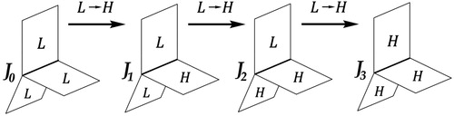
The aim of this work is to establish a method overcoming the restrictions of continuum modelling. Analysis on discrete complexes is proposed and used together with theoretical consideration of CDRX process. All TJs in our discrete model are boundaries of cell/grain faces. Figure 2 illustrates the TJ types formed and the possible transitions between these types as grain boundary type change from LAGB to HAGB during deformation. These transitions are not of the same probability, and are potentially material-dependent, which gives nontrivial evolution of TJs structure for given GBs type evolution function.

Figure 2. Schematic of the main triple junction types J_i with transitions due to change of one incident boundary from LAGB (L) to HAGB (H).

In Section 2 we will describe the model of the microstructure as a combinatorial complex and will outline the method used for analysis of its components. In Section 3 we will present results comparing the model performance with known analytical methods, develop strategies for transitions between grain boundary types, and demonstrate that the results obtained are in very good agreement with the experimental data [4] shown in Figure 1.

2. Model and method

The structures of 3D polycrystalline materials can be described by combinatorial complexes, which in the terminology of algebraic topology [23] are 3-complexes containing: 3-cells (cells), representing grains; 2-cells (faces) as boundaries of 3-cells, representing grain boundaries; 1-cells (edges) as boundaries of 2-cells, representing triple lines or junctions; and 0-cells (nodes) as boundaries of 1-cells, representing quadruple points. Such a combinatorial representation does not involve any metric information, i.e. sizes or shapes (flat or curved) of different cells, hence it is very suitable for analysis of sub-structures formed by different k-cells (k = 0,1,2,3) at any required length scale. The combinatorial complex can be embedded in a given metric space, for example R³, by providing coordinates of 0-cells with respect to fixed coordinate system and assuming flatness of all types of cells. This is not necessary for the analysis of sub-structures in our work, but we will use embedding for construction and visualisation purposes.

The structure of a combinatorial 3-complex is fully determined by three incidence matrices describing relations between 0-cells and 1-cells, between 1-cells and 2-cells, and between 2-cells and 3-cells, respectively. When the cells of a 3-complex are assigned orientations, the incidence matrices are rectangular with numbers 0, 1, −1, which allows for using them as discrete exterior derivatives [23]. For the purposes of this work, we define the incidence matrices differently: the elements of an incident matrix D relating k-cells and l-cells ($l>k$) are given by $d_{ij}=1$ when the ith k-cell is on the boundary of the jth l-cell, and $d_{ij}=0$ otherwise. Further, we define an auxiliary description of a combinatorial 3-complex via an adjacency matrix, A, which is a square matrix describing relations between k-cells only, and a diagonal matrix, G, describing the degree of a given k-cell, i.e. the number of neighbouring k-cells. The relation between the incidence matrix and the two auxiliary matrices is given by Grady and Polimeni [23](1) $A=D\cdot D^T-G.$(1) These matrices are extensively used in our analyses to determine neighbours and boundary elements, as well as to decide which TJs are changing their types when a LAGB changes to a HAGB.

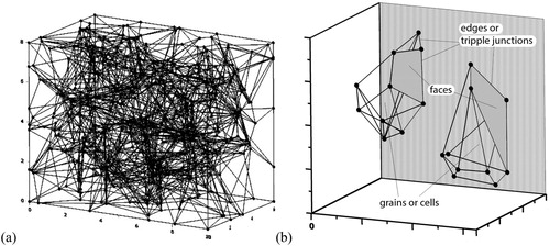
Combinatorial 3-complexes representing polycrystalline microstructures are constructed by a constrained Voronoi tessellation around given set of points distributed randomly in a given container. Free software Voro++ [24] is used for the tessellation. The Voro++ output is a list of nodes forming the Voronoi cells (polytops) together with the nodal coordinates. This allows for visualising the assembly and for obtaining statistical information, i.e. the number of vertices contained in each grain. Illustration of a discrete assembly containing 100 grains and a couple of separate polytopes is shown in Figure 3. A purpose built code, VoroC++Analyzer (VCA) [25], has been developed and used to post-process the results from Voro++ and construct all incidence, adjacency and diagonal matrices required for subsequent analysis of sub-structures.

Figure 3. A discrete complex with 100 grains (a) and a couple of Voronoi cells (b) with their elements.

We denote a 3-complex representing a microstructure by K. Generally, if the k-cells (k = 0,1,2,3) of K are equipped with some physical characteristics, which change as a result of a physical process, the purpose of the analysis is to predict how this process changes the connectivity characteristics of the 3-complex. Our calculations have shown that when the number of cells increases all relationships between variables defined on K elements approach a limit, which can be considered as their ‘infimum-complex’ values with acceptable accuracy. As an example, for the fraction $f_1$, the differences between the values obtained by 10, 30 and 100-cell complexes with 300-cell complex are about 50%, 25% and less than 1% respectively. This suggested that additional increase in the number of grains was not essential for our consideration and for saving computational time complexes with 300 grains were subsequently considered.

The process of CDRX at SPD is described as an evolution of parameters associated with various k-cells. Specifically, bulk dislocation density is assigned to 3-cells [11], grain boundary type is assigned to 2-cells, and triple line type is assigned to 1-cells. During SPD, changes of bulk dislocation density yields changes of HAGBs fraction p, which causes changes of $f_i$ [11]. In our consideration, we shall extensively use three experimental facts [11,19]: (1) the evolution of dislocation cell structure is much faster than the evolution of grain boundary structure; (2) dislocation cells are formed after initial collapse (at strain ∼0.3) and their sizes remain practically constant with increased deformation; and (3) at high accumulated strain, the grain size approaches asymptotically the dislocation cell size. These allow us to consider the dislocation cell structure after the initial collapse as our initial discrete complex K containing only LAGBs, i.e. p = 0. This initial condition agrees with all experiments [11], where even after the first SPD pass (at strain ∼0.4) the initial p of ∼0.9, typical for coarse grained materials, drastically decreases to almost zero due to the formation of new dislocation cell structure.

Starting with such an initial complex, at each deformation step, the type of certain 2-cells (grain boundaries) is changed from LAGBs to HAGBs in order to achieve the p corresponding to this strain level. For our simulations, the relationship p-accumulated strain is taken from a theoretical fitting of the experimental data [26] of the SPD process of copper alloys. This function, unique for each material, is the only material characteristic used in the simulations in this work. Generally, the fraction of HAGBs could be expressed as an order parameter for which the Landau theory [27] gives(2) $\dot{p}=\gamma \frac{\mathrm{\partial }F}{\mathrm{\partial }p}\simeq Ap-B{p}^3+C{p}^6,$(2) where the expansion of the free energy $F=F_0+A^{\mathrm{\prime }}{p}^2-B^{\mathrm{\prime }}{p}^4+C^{\mathrm{\prime }}{p}^6-\cdots$ contains only even degrees of $p$, $F_0$ is the free energy at $p=0$, $\gamma ,A,B,C,A^{\mathrm{\prime }}=A/2\gamma ,B^{\mathrm{\prime }}=B/4\gamma ,C^{\mathrm{\prime }}=C/6\gamma$ are empirical constants. For the initial stages of deformation, the first two terms completely determine the system behaviour. Integration of (2) with only the two first terms (noting that $p$ is always positive) leads to a logistic type of equation with the initial quasi-linear growth and subsequent saturation:(3) $p=\frac{\sqrt{A}\exp \left(A\epsilon \right)}{\sqrt{1+B\exp \left(2A\epsilon \right)}}-\sqrt{\frac{A}{1+B}}.$(3)

Here $A$ mainly affects the inflexion point of the curve, the saturation level is equal to $p_{SAT}=\sqrt{A/B}\le 1$ and the last term $\sqrt{A/1+B}$ satisfies the natural condition $p=0$ at $\epsilon =0$. The best approximation, accounting the next terms in the energy expansion, is(4) $p=\frac{\sqrt{A}\exp \left(A\epsilon \right)}{\sqrt{1+B\exp \left(2A\epsilon \right)}}+C\ln (1+\epsilon )-\sqrt{\frac{A}{1+B}}.$(4) Figure 4 shows a plot of Equation (3) with the parameters $A=2$, $B=0.9$ and of Equation (4) with $A=2$, $B=1.8$, $C=0.2$. The average curve for the experimental points [26] starts from $\epsilon \sim 1$, which corresponds to the average deformation after the first pass of equal-channel angular pressing (ECAP) [10,16]. Calculated curves have been shifted to the same initial point.

Figure 4. The average curve for experimental points [26] and its theoretical fitting by the Equations (3) and (4) with parameters $A=2$, $B=0.9$ and $A=2$, $B=1.8$, $C=0.2$ respectively.

There are different possibilities for the selection of LAGBs to be converted to HAGBs at each deformation step. The simplest one is random selection of a set of LAGBs. Once a 2-cell is converted to HAGB each of its boundary 1-cells (TJs) changes type from J_i to J_i+1. By generating the required number of new HAGBs, and changing TJs types using the edge-face incidence matrix, all fractions $f_i$ are calculated as functions of the accumulated strain value. This option will be tested firstly against existing theoretical models in the next section. Another possibility is to use a more process-informed selection for new HAGBs. In particular, the probability of an LAGB to become a new HAGB must be higher for LAGBs that already have HAGBs neighbours, i.e. a LAGB near a HAGB must be prone to become a new HAGB, because HAGBs usually act as local stress concentrators and have long-range surrounding elastic fields. This is expected to facilitate dislocation processes in their vicinity with simultaneous decrease of the activation energies for microstructural processes. The localisation of deformation on micro-level inside shear bands is another reason to change this selection. Furthermore, crystallography restrictions must prevent purely random distribution of HAGBs [22]. A couple of variants for such a selection will be explored in the next section in light of existing theories and experimental results.

3. Results and discussion

There are several theories for calculating TJs fractions as functions of HAGBs fraction in metals. The simplest one and advanced variants were discussed in Frary and Schuh [22]. We consider an advanced option that takes into consideration crystallographic constraints: if one or two boundaries adjacent to a TJ have a known type, HAGBs or LAGBs, there exist a limited range of misorientations for the remaining boundaries adjacent to the same TJ. This leads to the following functions for the TJ fractions [22] (using our notations for $f_i$):(5) $\begin{array}{rl}{f}_0=& \left(1-{\mathrm{\Pi }}_0^0\right)\left(1-{\mathrm{\Pi }}_0^1\right)\left(1-{\mathrm{\Pi }}_0^2\right)\\ f_1=& {\mathrm{\Pi }}_0^0\left(1-{\mathrm{\Pi }}_1^1\right)\left(1-{\mathrm{\Pi }}_1^2\right)+\left(1-{\mathrm{\Pi }}_0^0\right){\mathrm{\Pi }}_0^1\left(1-{\mathrm{\Pi }}_1^2\right)+\left(1-{\mathrm{\Pi }}_0^0\right)\left(1-{\mathrm{\Pi }}_0^1\right){\mathrm{\Pi }}_0^2\\ f_2=& {\mathrm{\Pi }}_0^0{\mathrm{\Pi }}_1^1\left(1-{\mathrm{\Pi }}_2^2\right)+{\mathrm{\Pi }}_0^0\left(1-{\mathrm{\Pi }}_1^1\right){\mathrm{\Pi }}_1^2+\left(1-{\mathrm{\Pi }}_0^0\right){\mathrm{\Pi }}_0^1{\mathrm{\Pi }}_1^2\\ f_3=& {\mathrm{\Pi }}_0^0{\mathrm{\Pi }}_1^1{\mathrm{\Pi }}_2^2\end{array}$(5) where ${\mathrm{\Pi }}_j^i$ are the local transition probabilities. In these, $i=0\dots 2$ is the number of boundaries that have been already assigned, and $j\le i$ is the number of these boundaries that have been classified as HAGBs. The equations for all ${\mathrm{\Pi }}_j^i$ have been derived in Frary and Schuh [22]. For the random case, i.e. not accounting for crystallographic constraints, all ${\mathrm{\Pi }}_j^i=p$ [22]. In such case Equation (5) transforms to:(6) $f_0=(1-p{)}^3;f_1=3p(1-p{)}^2;f_2=3p^2\left(1-p\right);f_3=p^3.$(6)

Figure 5 illustrates calculations of $f_i$ as functions of p based on the two theories. Each symbol corresponds to an analytical calculation, using Equation (5) or (6), for p obtained from the function of accumulated strain at SPD of copper alloys derived in Borodin and Bratov [11]. The curves were obtained with a discrete complex with 300 grains using purely random conversion of LAGBs to new HAGBs. The results appeared to be close to those from the two theories. The largest discrepancies arise in the behaviour of $J_2$ and $J_3$ curves on the initial deformation stages. This is partially due to the finite size of the discrete complex. This suggests that such random conversion is natural for a quasi-homogenous CDRX process. Differences between the two theories (5) and (6) for the SPD case are not very large, and can be practically neglected for $J_0$ and $J_3$. It is important to note, that by homogeneity of our random process we mean that the distribution of properties in the elements of the graph, representing the grain boundaries’ network, lacks observable structure, i.e. can be seen as homogeneous. The random process itself generates, undoubtedly, normal distribution of the selected number of grains, which is even more intricate, according to the rule of element enumeration in the discrete complex.

Figure 5. TJs fractions as functions of accumulated strain during SPD of copper alloys, obtained by discrete complex calculations (curves), calculations with random distribution of HAGBs (empty symbols), and with account for crystallographic constraints (filled symbols) [22].

Let us consider the probabilities for LAGBs to become new HAGBs to depend on the conversion of triple line types. In order to formalise this, we assign probabilities ${\alpha }_i={\alpha }_i\left(p\right)$, $i=0,1,2,3$ to the triple line types $J_1,J_2$ and $J_3$, respectively. For a given LAGB we denote by $T_i$, $i=0,1,2,3$, the number of its triple lines of type $J_i$, and introduce a grain boundary index(7) $G{B}_{ind}={\alpha }_1{T}_0+{\alpha }_2{T}_1+{\alpha }_3{T}_2,$(7) which expresses the changes in the LAGB neighbourhood if it were to be converted to HAGB. Upon such a conversion all adjacent TJs change their types from $J_{i-1}$ to $J_i$, $i=1,2,3$. So, the probabilities ${\alpha }_i$ represent affinities for conversion from $J_{i-1}$ to $J_i$, $i=1,2,3$ in the system.

To find ${\alpha }_i$ as functions of the grain boundary fraction we note that $p$ is the probability of a boundary to be HAGB [22] at a certain stage of the SPD process. Hence, the conversion probabilities ${\alpha }_i$ are likelihoods for a TJ with a certain type $J_i$, at determined moment of the process, to change its type to $J_{i+1}$, when the specific incident grain boundary undergoes LAGB to HAGB transition with probability $\delta p$. The increment $\delta p$ is obtained as the probability for a grain boundary to become a new HAGB at the current stage of the deformation process. At least three boundaries must change their type to HAGB during the increment $\delta p$. Figure 2 illustrates this process. TJs of type $J_0$ can: became $J_1$ with probability $3p(1-p{)}^2$ or three times less if we are looking for the specific grain boundary; became $J_2$ with probability $3p^2\left(1-p\right)$ or three times less if we are looking for the specific grain boundary; or became $J_3$ with probability $p^3$. TJs of type $J_1$ can: became $J_2$ with probability $p\left(1-p\right)$, or became $J_3$ with probability $p^2$. Finally, TJs of type $J_2$ can became $J_3$ with probability $p$. Hence, for the case without crystallographic constraints:(8) $\begin{array}{rl}& {\alpha }_1=p(1-p{)}^2+p^2\left(1-p\right)+p^3\\ & {\alpha }_2=p\left(1-p\right)+p^2\\ & {\alpha }_3=p\end{array}$(8)

When crystallographic constraints are taken into account, the local transition probabilities become:(9) $\begin{array}{rl}{\alpha }_1=& \left({\mathrm{\Pi }}_0^0\left(1-{\mathrm{\Pi }}_1^1\right)\left(1-{\mathrm{\Pi }}_1^2\right)+\left(1-{\mathrm{\Pi }}_0^0\right){\mathrm{\Pi }}_0^1\left(1-{\mathrm{\Pi }}_1^2\right)+\left(1-{\mathrm{\Pi }}_0^0\right)\left(1-{\mathrm{\Pi }}_0^1\right){\mathrm{\Pi }}_0^2\right)/3\\ & +\left({\mathrm{\Pi }}_0^0{\mathrm{\Pi }}_1^1\left(1-{\mathrm{\Pi }}_2^2\right)+{\mathrm{\Pi }}_0^0\left(1-{\mathrm{\Pi }}_1^1\right){\mathrm{\Pi }}_1^2+\left(1-{\mathrm{\Pi }}_0^0\right){\mathrm{\Pi }}_0^1{\mathrm{\Pi }}_1^2\right)/3+{\mathrm{\Pi }}_0^0{\mathrm{\Pi }}_1^1{\mathrm{\Pi }}_2^2\\ {\alpha }_2=& \left(1\cdot {\mathrm{\Pi }}_1^1\left(1-{\mathrm{\Pi }}_2^2\right)+1\cdot \left(1-{\mathrm{\Pi }}_1^1\right){\mathrm{\Pi }}_1^2\right)/2+1\cdot {\mathrm{\Pi }}_1^1{\mathrm{\Pi }}_2^2\\ {\alpha }_3=& 1\cdot 1\cdot {\mathrm{\Pi }}_2^2.\end{array}$(9)

Here ${\mathrm{\Pi }}_0^0\left(1-{\mathrm{\Pi }}_1^1\right){\mathrm{\Pi }}_1^2$ represents the transformation of the first grain boundary (see Figure 2) with probability ${\mathrm{\Pi }}_0^0$. This is followed by retaining the type of the second boundary (adjacent to the first one) with probability $\left(1-{\mathrm{\Pi }}_1^1\right)$ and by transforming the third adjacent boundary with probability ${\mathrm{\Pi }}_1^2$. Other probabilities are explained in a similar way. For TJs of type $J_2$ we suppose that two boundaries are HAGBs with probability equal 1 and the third one – with ${\mathrm{\Pi }}_2^2$.

The LAGB that will be converted into HAGB, say $N_{HAGB}^o$, is selected to be the one maximising the following functional over the set $\text{B}$ of all LAGBs:(10) $N_{HAGB}^o\to \underset{\mathrm{B}}{max}\left\{G{B}_{ind}\left(k\right)\right\},\mathrm{\forall }k\in \text{B}.$(10) In practice, a transition probability index $G{B}_{ind}={\alpha }_1{T}_0+{\alpha }_2{T}_1+{\alpha }_3{T}_2$ is calculated for each LAGB and the LAGB with the highest index is converted to HAGB first. This process is repeated until the required p for the current calculation step is achieved. In the initial stage, the algorithm takes the first few boundaries randomly and proceeds in the way described above.

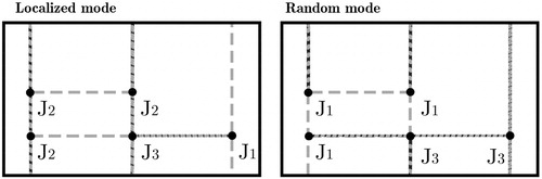
However, real grain structure evolution during SPD is often much more complicated and may not follow the homogeneous distribution implied by the analytical theory as illustrated by Figure 1. The recent experiments [4] have shown that $f_2$ and $f_3$ in Cu–Cr–Zr alloy are much higher than predicted theoretically. Correspondingly, because the sum of all fractions is one, $f_1$ is significantly lower, than the one predicted by the ‘homogeneous’ theory. Authors of [4,19] suggest that this happens due to micro-localisation process inside the grains during SPD of copper alloys. This type of localisation changes modes of continuous dynamic recrystallisation such that a significant number of new HAGBs form as shear bands inside the pre-existed grains. Figure 6 shows 2D sketches of localised and random distribution of seven grain boundaries. The picture illustrates that at localisation mode most of the TJs must have type $J_2$, then $J_3$ with an insignificant number of $J_1$ during the deformation process, while at random generation of GBs every node sometimes had a type $J_1$.

Figure 6. The sketch of triple junction distribution in the small area of a grain with the same number of boundaries and different distribution of TJ types. Dotted grey lines represent LAGBs, while all bold lines are HAGBs. Localised mode of CDRX must generate much less TJs with the only adjacent HAGB ($J_1$ type), than in any random process.

We take into consideration the effect of inhomogeneity in an empirical way. The GB index can be simply expressed by additional coefficients ${\lambda }_1,{\lambda }_2$:(11) $G{B}_{ind}={\alpha }_1{T}_0+{\lambda }_1{\alpha }_2{T}_1+{\lambda }_2{\alpha }_3{T}_2.$(11) As discussed earlier, localisation implies that the transition probabilities $J_1\to J_2$ and $J_2\to J_3$ must be greater than $J_0\to J_1$. The results for all J-curves at α _i obtained by Equation (9) are shown in Figure 7(a). Calculations with Equation (8) provide close results. Simulations with various λ _i have been performed and the best fit to experimental data has been found at λ₁ = 3 and λ₃ = 4. Comparing with the purely random case, the curves in Figure 7(b) calculated by Equation (11) with this selection of λ _i fit the experiments [4] qualitatively better: f₁ has been reduced almost twice with increase of f₂, f₃ and similar values of f₀.

Figure 7. Calculation curves of TJs fractions with the discrete complex approach, obtained for (a) quasi-homogeneous distribution of TJs by Equation (9) and (b) including micro-inhomogeneity phenomena by Equation (11) with ${\lambda }_1=3$, ${\lambda }_2=4$. Experimental points have been taken from Morozova et al. [4].

Even better agreement with experimental results could be obtained by totally empirical way with the constant ${\alpha }_i$ coefficients ${\alpha }_1=1,{\alpha }_2=10$ and ${\alpha }_3=5$, that is shown in Figure 8.

Figure 8. Calculation of TJs fractions with the discrete complex approach by Equation (8) with the constant values ${\alpha }_1=1,{\alpha }_2=10$ and ${\alpha }_3=5$. Experimental points have been taken from Morozova et al. [4].

This approach allows for improving the theoretical consideration of CDRX process in metals during SPD. The usual equation for average dislocation cells size evolution has the form [11](12) $D=\frac{\text{β}}{\sqrt{{\rho }_D}},$(12) where the coefficient $\text{β}\sim 10$ depends on the material, ${\rho }_D$ is the scalar dislocations density (total dislocation length per unit volume). A comprehensive discussion about the physical meaning of $\text{β}$ is in the works of Galindo-Nava with Rivera-Dıaz-del-Castillo [28,29]. Unfortunately, this simple equation does not work for the CDRX process [11]. Strictly speaking, to predict grain size evolution, d, in the same way as the cell size evolution, D, the parameter $\text{β}$ must became a function, not a constant [30]. As in experiments [4] cell sizes refer to the distances between low angle dislocation boundaries, while grain sizes to distances between HAGBs boundaries, the most natural way to define the second value is(13) $d=\frac{D}{p}.$(13) Here homogeneous distribution of HAGBs boundaries through the material is implicitly assumed. There is no way to predict the effect of their inhomogeneity by means of one scalar parameter. According to our previous analysis of triple junctions’ network, we propose a new, more informative, way to describe CDRX. If one considers the distances between TJs (or triple lines in 3D) as a measure of average grain size, Equation (13) can be modified for slightly inhomogeneous microstructure as(14) $d=\frac{3D}{f_1+2f_2+3f_3}$(14) At homogeneous distribution of TJs, the substitution of Equation (6) into (14) turns the latter into Equation (13). Further, in the limit of fully random GB network $f_1=f_2=0;$ $f_3=1$, Equation (14) provides the expected equality $d=D$. Other possible junction types (not allowed in the complex constructed by Voronoi tessellation) such as $J_4$ for cube-like grains can be included into the $J_3$ fraction if another microstructure containing such types is considered. It needs to be clarified that in Equation (14) it is assumed that all types of TJs have essentially homogeneous distributions, while this is not required for the grain boundary types. Because of the inverse proportionality, Equation (14) provides a result just slightly differ from Equation (13). Localisation leads to some decrease of the average grain size during SPD in the beginning, which remains approximately constant at large accumulated strains [26]. This shows that completely different structures of grain boundaries can be hardly distinguished by only measuring the average grain size.

Another interesting possibility for our discrete approach is the prediction of a full connectivity matrix of the TJs system that is not within the reach of any continuum approach. Such a connectivity matrix can be considered as a homogeneity measure of TJs distributions and could be very useful, e.g. in the design of new materials with high electrical conductivity. Each element on the connectivity matrix $j_{ij}$ stands for fraction of TJs of type $J_i$ directly connected with TJs of type $J_j$, i.e. it reflects the number of junctions $j_{11}:J_1\leftrightarrow J_1$, $j_{12}:J_1\leftrightarrow J_2$, … etc. 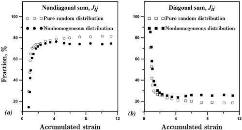Figure 9 shows results for different elements $j_{ii}={\sum }_k{j}_{kk}$ and $j_{ij}={\sum }_{k\ne l}{j}_{kl}$ obtained using the combinatorial tools from the previous section. There are two cases corresponding to purely random HAGBs evolution as in Figures 5 and 7(a), and to non-homogeneous evolution as in Figures 7(b) and 8. The inhomogeneity in copper alloys is clearly demonstrated by the differences in the connectivity characteristics, particularly after accumulated strain of approximately 4. The diagonal sum representing connectivity of junctions of the same type notably increases from the homogeneous to the non-homogeneous case, while the non-diagonal sum for $i\ne j$ correspondingly decreases. This outcome is a direct consequence of the new HAGBs generation approach, which has been demonstrated to be in good agreement with the available experimental data in Figure 7. It seems natural that in localised mode $J_2\leftrightarrow J_2$ and then $J_3\leftrightarrow J_3$ junctions must be much more common than in the random case (see Figure 6).

Figure 9. Purely random evolution of the TJs system and non-homogeneous evolution accounting micro-localisation processes. Sums of nondiagonal (a) and diagonal (b) components of the connectivity matrix.

Pervasive investigations of the connectivity matrix reveal the process dynamics, such as the appearance of a kernel and its surrounding development. In Table 1 data for both random and localised modes for two deformation levels are shown. All values $j_{ij}^{\mathrm{\prime }}$ given as fractions (in per cents) of $J_i\leftrightarrow J_j$, $i,j=\{0,1,2,3\}/\{i=j=0\}$ junctions from the total number of nonzero TJs. Other words, we did not take into account $J_0\leftrightarrow J_0$ junctions at these calculations, considering them just as a measure of deformation level. It is very useful to introduce the concept of a discrete complex kernel as the set of TJs with $J_2\leftrightarrow J_2,$ $J_2\leftrightarrow J_3$ and $J_3\leftrightarrow J_3$ links only. Along with that, one can define the density of links surrounded the kernel and neighbour TJs ($J_1\leftrightarrow J_2,$ $J_1\leftrightarrow J_3,$ $J_1\leftrightarrow J_1$) or its periphery. Finally, a number of $J_0\leftrightarrow J_1,$ $J_0\leftrightarrow J_2$ and $J_0\leftrightarrow J_3$ joints gives a set of TJs bounded by $J_0$ junctions.

Table 1. Nonzero TJs connectivity matrices for two different deformation stages at random and localised modes.

All the values $j_{ij}^{\mathrm{\prime }}$ are given as the fractions (in per cents) of corresponding $J_i\leftrightarrow J_j$, $i,j=\{0,1,2,3\}/\{i=j=0\}$ joints from the total number of nonzero TJs. The sizes of the kernels, peripheries and bounds have been calculated for all these cases.

In the random case, a kernel forms after the accumulated strain equal 3 that is obviously incorrect for SPD processes, where the new grain structure is appearing already at deformations about 2 [26]. More interesting that during the deformation process in all cases periphery changes just in fourth, while the bound decreases almost twice.

The result suggests that the TJ connectivity characteristics may play an important role in describing the microstructure evolution away from the simple random case, i.e. during non-homogeneous development. Based on the connectivity matrices one can generalised grain boundary index by introducing tensorial probabilities ${\alpha }_{ij}$, leading to(15) $G{B}_{ind}=\sum _{i,j=\{0,1,2,3\}}{\alpha }_{ij}{T}_{ij},$(15) where $T_{ij}$ are the numbers of $J_i\leftrightarrow J_j$ connections for a given grain boundary. It should be noted that there is no experimental data available at this point to compare the predicted TJ connectivity. Once such data becomes available, the proposed modelling approach in combination with the data will help providing explanations as to how these characteristics affect the evolution of material properties.

4. Conclusions

Discrete combinatorial complexes offer natural representations of the grain structures of polycrystalline solids. The analyses of any substructures and their evolution can be performed without recourse to metric information, i.e. irrespective of the sizes and shapes of grains and boundaries. Clearly, such metric information may play a role in probabilities of transforming LAGBs to HAGBs or to be a leading mechanism of micro-localisation. Size and shape of structural elements are important driving forces on microstructural evolution. In this work, we have postulated all changes heuristically, but the effects of size and shape are subject of ongoing model development. An important element of this work is the separation of purely combinatorial properties of the grains’ network from other physically motivated impacts, such as dimensional properties of the complex elements.

Here, we have constructed and analysed discrete complexes based on Voronoi space tessellation containing sufficient number of 3-cells (grains), 2-cells (GBs) and 1-cells (TJs) for the results to be considered representative for the evolution of physical processes defined on its elements. This has allowed us to overcome the limitations of continuous approach and to describe the effects of inhomogeneity on grain structure evolution as well as on triple junction’s network evolution in details.

Firstly, we have demonstrated that the discrete model with purely random evolution/selection of high-angle grain boundaries gives similar results as existing analytical predictions for such case [22]. This lends confidence to the model accuracy. Secondly, we have proposed a process for HAGBs evolution where the selection is based on the TJs-related functional maximisation, and have demonstrated that it provides a good fit to the experimental data for which the existence of inhomogeneities in Cu–Cr–Zr alloys is brightly manifested [4]. Thirdly, we have introduced substructure characteristic measuring the network of triple junctions, and have shown that these evolve differently for inhomogeneous cases compared to the random ones. Specifically, due to the inhomogeneity in copper alloys developed during SPD, the connectivity between TJs of the same type increases, while the connectivity between TJs of different types decreases in comparison to a homogeneous CDRX process. The proposed combinatorial approach is a useful tool for analysis of substructures during severe plastic deformations and combined with further experimental evidence should lead to explanations of how the changing structures are linked to the changing properties.

Acknowledgements

Authors appreciate highly the financial support of EPSRC via grant EP/N026136/1, thank Dr Odysseas Kosmas for many valuable discussions, and the reviewers for their significant contribution to the improvement of the manuscript. The authors confirm that the data supporting the findings of this study is available within the article. VCA code is available on the web-page [25].

Disclosure statement

No potential conflict of interest was reported by the authors.

Additional information

Funding

This work was supported by Engineering and Physical Sciences Research Council: [Grant Number EP/N026136/1 “Geometric Mechanics of Solids”].

References

- P. Ghosh, O. Renk, and R. Pippan, Microtexture analysis of restoration mechanisms during high pressure torsion of pure nickel, Mater. Sci. Eng. A. 684 (2017), pp. 101–109. doi: 10.1016/j.msea.2016.12.032
- S. Patala, J.K. Mason, and C.A. Schuh, Improved representations of misorientation information for grain boundary science and engineering, Prog. Mater. Sci. 57 (2012), pp. 1383–1425. doi: 10.1016/j.pmatsci.2012.04.002
- S. Kobayashi, T. Maruyama, S. Tsurekawa, and T. Watanabe, Grain boundary engineering based on fractal analysis for control of segregation-induced intergranular brittle fracture in polycrystalline nickel, Acta Mater. 60 (2012), pp. 6200–6212. doi: 10.1016/j.actamat.2012.07.065
- A. Morozova, E.N. Borodin, V. Bratov, S. Zherebtsov, A. Belyakov, and R. Kaibyshev, Grain refinement kinetics in a low alloyed Cu–Cr–Zr alloy subjected to large strain deformation, Materials 10 (2017), pp. 1394. doi: 10.3390/ma10121394
- T. Sakai, A. Belyakov, R. Kaibyshev, H. Miura, and J.J. Jonas, Dynamic and post-dynamic recrystallization under hot, cold and severe plastic deformation conditions, Prog. Mater. Sci. 60 (2014), pp. 130–207. doi: 10.1016/j.pmatsci.2013.09.002
- G.S. Rohrer, Measuring and interpreting the structure of grain-boundary networks, J. Am. Ceram. Soc. 94(3) (2011), pp. 633–646. doi: 10.1111/j.1551-2916.2011.04384.x
- M. Li and T. Xu, Topological and atomic scale characterization of grain boundary networks in polycrystalline and nanocrystalline materials, Prog. Mater. Sci. 56 (2011), pp. 864–899. doi: 10.1016/j.pmatsci.2011.01.011
- G.S. Rohrer and H.M. Miller, Topological characteristics of plane sections of polycrystals, Acta Mater. 58 (2010), pp. 3805–3814. doi: 10.1016/j.actamat.2010.03.028
- T. Wanner, E.R. Fuller Jr, and D.M. Saylor, Homology metrics for microstructure response fields in polycrystals, Acta Mater. 58 (2010), pp. 102–110. doi: 10.1016/j.actamat.2009.08.061
- A. Vinogradov and Y. Estrin, Analytical and numerical approaches to modelling of severe plastic deformation, Prog. Mater. Sci. 95 (2018), pp. 172–242. doi: 10.1016/j.pmatsci.2018.02.001
- E.N. Borodin and V. Bratov, Non-equilibrium approach to prediction of microstructure evolution for metals undergoing severe plastic deformation, Mater. Charact. 141 (2018), pp. 267–278. doi: 10.1016/j.matchar.2018.05.002
- A. Morozova and R. Kaibyshev, Grain refinement and strengthening of a Cu–0.1Cr–0.06Zr alloy subjected to equal channel angular pressing. Philos. Mag. 97 (2017), pp. 2053–2076. doi: 10.1080/14786435.2017.1324649
- A. Vinogradov, Mechanical properties of ultrafine-grained metals: new challenges and perspectives, Adv. Eng. Mater. 17 (2015), pp. 1710–1722. doi: 10.1002/adem.201500177
- V. Bratov and E.N. Borodin, Comparison of dislocation density based approaches for prediction of defect structure evolution in aluminium and copper processed by ECAP, Mat. Sci. Eng. A. 631 (2015), pp. 10–17. doi: 10.1016/j.msea.2015.02.019
- I. Sabirov, M.Y. Murashkin, and R.Z. Valiev, Nanostructured aluminium alloys produced by severe plastic deformation: new horizons in development, Mat. Sci. Eng. A. 560 (2013), pp. 1–24. doi: 10.1016/j.msea.2012.09.020
- R.Z. Valiev, R.K. Islamgaliev, and I.V. Alexandrov, Bulk nanostructured materials from severe plastic deformation, Prog. Mat. Sci. 45 (2000), pp. 103–189. doi: 10.1016/S0079-6425(99)00007-9
- R. Pippan, S. Scheriau, A. Taylor, M. Hafok, A. Hohenwarter, and A. Bachmaier, Saturation of fragmentation during severe plastic deformation, Annu. Rev. Mater. Res. 40 (2010), pp. 319–343. doi: 10.1146/annurev-matsci-070909-104445
- I.J. Beyerlein and L.S. Tóth, Texture evolution in equal-channel angular extrusion, Prog. Mater. Sci. 54 (2009), pp. 427–510. doi: 10.1016/j.pmatsci.2009.01.001
- A. Belyakov, T. Sakai, H. Miura, and K. Tsuzaki, Grain refinement in copper under large strain deformation, Phil. Mag. A 81 (2001), pp. 2629–2643. doi: 10.1080/01418610108216659
- E.N. Borodin and A.E. Mayer, Localization of plastic flow at dynamic channel angular pressing, Tech. Phys. 58(8) (2013), pp. 1159–1163. doi: 10.1134/S1063784213080070
- E.N. Borodin and A.E. Mayer, Structural model of mechanical twinning and its application for modeling of the severe plastic deformation of copper rods in Taylor impact tests, Int. J. Plast. 74 (2015), pp. 141–157. doi: 10.1016/j.ijplas.2015.06.006
- M. Frary and C.A. Schuh, Percolation and statistical properties of low- and high-angle interface networks in polycrystalline ensembles, Phys. Rev. B. 69 (2004), pp. 134115. doi: 10.1103/PhysRevB.69.134115
- L.J. Grady and J.R. Polimeni, Discrete Calculus, Springer-Verlag, London, 2010.
- Voro++ free software available at http://math.lbl.gov/voro++
- VoroC++Analyzer (VCA) is available for free at https://mapos.manchester.ac.uk
- E.N. Borodin, A. Morozova, V. Bratov, A. Belyakov, and A.P. Jivkov, Experimental and numerical analyses of microstructure evolution of Cu-Cr-Zr alloys during severe plastic deformation, Mater. Charact. 156 (2019), pp. 109849. doi: 10.1016/j.matchar.2019.109849
- E.M. Lifshitz and L.P. Pitaevskii, Physical Kinetics: Volume 10 (Course of Theoretical Physics), Butterworth Heinemann, Oxford, 1981.
- E.I. Galindo-Nava and P.E.J. Rivera-Dıaz-del-Castillo, A thermodynamic theory for dislocation cell formation and misorientation in metals, Acta Mater. 60 (2012), pp. 4370–4378. doi: 10.1016/j.actamat.2012.05.003
- E.I. Galindo-Nava and P.E.J. Rivera-Dıaz-del-Castillo, Modelling plastic deformation in BCC metals: dynamic recovery and cell formation effects, Mater. Sci. Eng., A 558 (2012), pp. 641–648. doi: 10.1016/j.msea.2012.08.068
- R. Lapovok, F.H. Dalla Torre, J. Sandlin, C.H.J. Davies, E.V. Pereloma, P.F. Thomson, and Y. Estrin, Gradient plasticity constitutive model reflecting the ultrafine micro-structure scale: The case of severely deformed copper, J. Mech. Phys. Solids. 53 (2005), pp. 729–747. doi: 10.1016/j.jmps.2004.11.006