Equilibrium states of confined ions in two dimensions

ABSTRACT

Ions that are trapped in two dimensions and are subject to a harmonic confining potential have widely varying stationary states that exhibit various asymptotic forms and bifurcations. We present a ‘birds-eye’ view of these structures for N = 2 to 5 ions, and the full range of anisotropy. These results may be interrogated in detail using the software provided here. Energy variations at bifurcation points and limits are also identified; for N = 5 these include blue-sky (or saddle-node) bifurcations. A limited attempt is also made to explore such features for a larger system of ions, i.e. N = 10.

KEYWORDS:

• Computation
• computer modelling
• morphology

1. Introduction

There is an extensive, if fragmentary, literature on the structure of 2d ion crystals. By this, we mean systems of identical ions confined by transverse harmonic potentials to two dimensions in two orthogonal directions and interacting with each other via a Coulomb potential. In practice, ion crystals can be realised by the use of a Penning trap [1–5]. Interest in such systems has been driven by the proposal that trapped ions can offer a practical system for quantum computing [6]. Similar structures can also be obtained in systems of charges interacting via Yukawa (or screened) potentials [7].

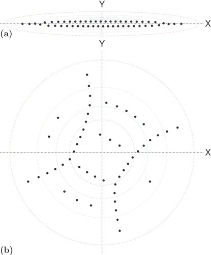
Ion crystals are found to have a wide variety of equilibrium states, depending on the anisotropy of the confining potential [1,2,4,8,9]. Examples of calculations taken from results presented in later sections are shown in Figure 1. The enumeration and description of these states presents a challenge to computation which has previously been taken up only to a limited extent [10]. Here we embark on an exploration of the rich and complex scenario of the general problem.

Figure 1. (a) Example of a computed stable arrangement of fifty ions (shown as black dots) trapped in an anisotropic harmonic potential of the form $\frac{1}{2}(k_x{x}^2+k_y{y}^2)$ with $k_y>>k_x$. Here the anisotropy parameter $\lambda =0.97$ – see Section 2 for the definition. (b) An unstable equilibrium arrangement of fifty ions in an isotropic harmonic potential (i.e. $k_x=k_y$ or $\lambda =0$). In both figures the contours are lines of increasing equipotential (from indigo to red). For further details see Section 4.

Experimental work that dates back to at least 1992 [8] includes the case of a linear chain (i.e. the limit of extreme anisotropy). This undergoes a zigzag instability (similar to that seen in Figure 1(a)), as the confining potential in the transverse direction is relaxed. In the opposite extreme Bedanov and Peeters [11] and Bolton and Rössler [12] investigated the lowest energy solutions for an isotropic confining potential, for large numbers of ions. Rancova et al. [13] explored and elucidated some structural transitions for small numbers.

More recently, interest in the use of trapped ions for quantum computing [14] has stimulated further computations, mainly of the ‘kinks’ which may be found in the zigzag chain [10,15]. Figure 1 of the paper by Landa et al. [10] gives an impression of the complexity of this subject. It is a bifurcation diagram for 31 ions, including various bifurcations relating to the generation of kinks, as the initially strong radial confinement, resulting in a linear chain, is progressively relaxed. This is the most comprehensive diagram which has so far been advanced. It is confined to a narrow regime and is a schematic sketch (although some quantitative information is included).

Our main contribution in the present paper is to take a wider view of the subject. For a small number N of ions all of the (stable and unstable) equilibrium solutions are presented (up to N = 5) for the full range of anisotropy. We do so in terms of a diagram whose two axes are scaled energy $E^{\ast }\left(\lambda \right)$ and an anisotropy parameter λ which varies from $\lambda =0$ (the isotropic case) to $\lambda =1$ (the anisotropic limit).

The large number and wide variety of equilibrium structures is a challenge to presentation, which we meet by the use of interactive notebooks which will enable the reader to interrogate the results and explore particular structures. Some of the structures found in the myriad of possibilities are remarkably elegant and give the subject an aesthetic as well as a scientific appeal. Figure 1(b) presents an example, an unstable equilibrium configuration for a system of fifty ions.

Our initial aim is to map out all of the stable and unstable equilibrium configurations for N = 2, 3, 4 and 5 in terms of their values of energy and anisotropy. We present less comprehensive results for N = 10.

We intend to do more than push back the frontiers of what is computationally achievable: we hope to provide an extensive semi-analytic framework of understanding as well. In doing so we are not confined to the stable equilibrium states; we also map out the unstable states. While unstable equilibrium states may not be readily accessible in experiment, they are nevertheless important in constructing a bifurcation diagram (representing the energy, position or any other parameter of equilibrium structures as a function of the confining potential).

In the following sections, we give basic definitions and first examine the trivial case of N = 2. We have recourse to numerical methods for larger values of N. We also examine and analyse various parts of the diagram, such as those involving bifurcation points (including blue-sky bifurcations).

Given the wealth of detail, it should prove helpful that we have developed a computational tool (based on Mathematica) with which the reader may interrogate the results (see hyperlinks in the various bifurcation diagrams shown below). The notebooks for N = 2, 3 and 4 can be displayed and interrogated using the links provided in the text. The case of N = 5 is too complex to be displayed in this way. Instead, we recommend that the user downloads a free copy of the Wolfram Player [16] to increase the responsiveness of the notebooks.

2. Definition of the problem and scaling property

The total energy E of a cluster of N charges Q, confined by a $2d$ harmonic potential, is given by (1) $E=\frac{1}{2}\sum _i^N(k_x{X}_i^2+k_y{Y}_i^2)+\frac{Q^2}{4\pi {ϵ}_0}\sum _{i<j}^N\left[\right(X_i-X_j{)}^2+(Y_i-Y_j{)}^2{]}^{-1/2},$(1) where $X_i$ and $Y_i$ are the Cartesian coordinates of the ith charge, while $k_x$ and $k_y$ are the force constants for the harmonic confining potential in the x and y directions, respectively. Note that the limits $k_x\to 0$ or ∞ (or similarly for $k_y$) take us to confined linear systems, while $k_x=k_y$ defines an isotropic potential. For convenience, we use $a=\frac{Q^2}{4\pi {ϵ}_0}$ (${ϵ}_0$ is the permittivity of free space) in what follows.

The equilibrium values of E are dependent on $k_x$, $k_y$, and a, and are invariant under $k_x\lessgtr k_y$. Hence E is a function of a, $(k_x+k_y)$, $k_x/k_y$. The last represents the anisotropy of the potential and has been used by others (e.g. [10,17]), but we prefer to use (2) $\lambda =\frac{|k_x-k_y|}{k_x+k_y},$(2) which is a measure of the anisotropy of the potential, symmetric in $k_x$ and $k_y$.

Since the parameter a has the dimension of energy × length, while $k_x$ and $k_y$ have the dimensions of energy/length${}^2$ and λ is dimensionless, it follows that the energy must take the form (3) $E=(k_x+k_y{)}^{1/3}{a}^{2/3}{E}^{\ast },$(3) where $E^{\ast }$ is a function of λ only, specified below (Equation (4(4) $\begin{array}{r}{E}^{\ast }\left(\lambda \right)=\frac{(1-\lambda )}{4}\sum _i^N{x}_i^2+\frac{(1+\lambda )}{4}\sum _i^N{y}_i^2+\sum _{i<j}^N\left[\right(x_i-x_j{)}^2+(y_i-y_j{)}^2{]}^{-1/2},\end{array}$(4) )).

The dimensionless scaled energy $E^{\ast }$ is the quantity that we will compute and present in the following sections. It may be rescaled in any particular case using the above relation.

The goal is to find equilibrium states (and their energy) as a function of λ, where $\lambda =0$ and $\lambda =1$ represent the isotropic and extreme anisotropic cases, respectively. (See also Figure 1 for contours of constant equipotential for two different values of λ.)

3. The elementary case of N = 2

The case of two charges in a harmonic potential is easily treated analytically and it is instructive to examine it in detail, containing as it does, some key features of the more complex diagrams for higher N.

The dimensionless energy $E^{\ast }\left(\lambda \right)$ of Equation (3(3) $E=(k_x+k_y{)}^{1/3}{a}^{2/3}{E}^{\ast },$(3) ) is readily evaluated as (4) $\begin{array}{r}{E}^{\ast }\left(\lambda \right)=\frac{(1-\lambda )}{4}\sum _i^N{x}_i^2+\frac{(1+\lambda )}{4}\sum _i^N{y}_i^2+\sum _{i<j}^N\left[\right(x_i-x_j{)}^2+(y_i-y_j{)}^2{]}^{-1/2},\end{array}$(4) where the $x_i$ and $y_i$ are dimensionless quantities, with $X_i=(\frac{a}{k_x+k_y}{)}^{1/3}{x}_i$, $Y_i=(\frac{a}{k_x+k_y}{)}^{1/3}{y}_i$. (Without loss of generality we have chosen $k_y>k_x$ here, as was done in our simulations.)

Let the first charge be located at, (5) $(x_1,y_1)=\delta (\cos \theta ,\sin \theta ),$(5) where δ is the distance from the centre of the system and θ is the polar angle. For reasons of equilibrium and symmetry, the second charge must be located at, (6) $(x_2,y_2)=\delta (\cos (\theta +\pi ),\sin (\theta +\pi \left)\right)=-(x_1,y_1).$(6) From these coordinates and Equation (4(4) $\begin{array}{r}{E}^{\ast }\left(\lambda \right)=\frac{(1-\lambda )}{4}\sum _i^N{x}_i^2+\frac{(1+\lambda )}{4}\sum _i^N{y}_i^2+\sum _{i<j}^N\left[\right(x_i-x_j{)}^2+(y_i-y_j{)}^2{]}^{-1/2},\end{array}$(4) ) (expressed in polar coordinates δ and θ), we can write down the (dimensionless) energy $E^{\ast }$ for a system of two charges. To obtain the stationary states we apply the conditions $\frac{d{E}^{\ast }}{d\theta }=0$ (yielding the two solutions $\theta =0$ and $\theta =\pi /2$) and $\frac{d{E}^{\ast }}{d\delta }=0$, resulting in (7) $E^{\ast }=\{\begin{array}{cc}{\displaystyle \frac{3}{2^{5/3}}(1-\lambda ),}& \mathrm{i}\mathrm{f}\theta =0,\\ {\displaystyle \frac{3}{2^{5/3}}{(1+\lambda )}^{1/3},}& \mathrm{i}\mathrm{f}\theta =\pi /2.\end{array}$(7) These values and their corresponding ion arrangements are shown in Figure 2,which plots energy $E^{\ast }\left(\lambda \right)$ of the solutions against the anisotropy parameter λ, ranging from zero (the isotropic case) to unity (the limit of anisotropy). The images adjacent to Figure 2 identify examples of structures for $\lambda =0$ and $\lambda =0.8$.

Figure 2. Bifurcation diagram, in terms of scaled energy E* and anisotropy parameter λ, for N = 2. In the isotropic limit $\lambda =0$ there is only one solution $I1$ which is rotationally degenerate. For finite anisotropy (i.e. $0<\lambda \le 1$) there are two solutions, labelled $A1$ and $A2$. For an interactive version of this figure see [18]. Note, in the bifurcation diagram, stable equilibrium solutions are indicated in blue, while unstable equilibrium solutions are indicated in black. All images of structures are plotted using dimensionless coordinates (i.e. positions are scaled by $L_0=\left(a/\right(k_x+k_y){)}^{1/3}$). The configuration shown on the left is for $\lambda =0$, while $\lambda =0.8$ for the configurations shown on the right.

For the isotropic state ($\lambda =0$) Equation (7(7) $E^{\ast }=\{\begin{array}{cc}{\displaystyle \frac{3}{2^{5/3}}(1-\lambda ),}& \mathrm{i}\mathrm{f}\theta =0,\\ {\displaystyle \frac{3}{2^{5/3}}{(1+\lambda )}^{1/3},}& \mathrm{i}\mathrm{f}\theta =\pi /2.\end{array}$(7) ) yields, (8) $E^{\ast }=3/2^{5/3}\sim 0.945$(8) for both $\theta =0$ and $\theta =\pi /2$. The solution consists of a pair of points, as shown in Figure 2 (structure labelled $I1$), and is in fact degenerate with respect to any rotation.

It can be seen from Equation (7(7) $E^{\ast }=\{\begin{array}{cc}{\displaystyle \frac{3}{2^{5/3}}(1-\lambda ),}& \mathrm{i}\mathrm{f}\theta =0,\\ {\displaystyle \frac{3}{2^{5/3}}{(1+\lambda )}^{1/3},}& \mathrm{i}\mathrm{f}\theta =\pi /2.\end{array}$(7) ) that anisotropy (i.e. $\lambda >0$) dictates that there are two distinct solutions (these are also shown in Figure 2 and are labelled $A1$ and $A2$), with the two charges orientated respectively parallel ($\theta =0$) and perpendicular ($\theta =\pi /2$) to the x-axis, the former stable, indicated in blue, and the latter unstable (recall $k_x\le k_y$), indicated in black. In the anisotropic limit ($\lambda =1$) we obtain (9) $E^{\ast }=\{\begin{array}{cc}0,& \mathrm{i}\mathrm{f}\theta =0,\\ 3/2^{4/3}\tilde{1}.191,& \mathrm{i}\mathrm{f}\theta =\pi /2.\end{array}$(9)

4. Computational methods

For values N > 2 such direct calculations become impractical and we resort to numerical methods. Equilibrium states may be found in various ways; we describe two methods below. Calculations may be made for any chosen $k_x$, $k_y$ and a and rescaled to give $E^{\ast }$ and λ (see Section 2).

Stable equilibrium states may be obtained by direct minimisation of energy (Equation (4(4) $\begin{array}{r}{E}^{\ast }\left(\lambda \right)=\frac{(1-\lambda )}{4}\sum _i^N{x}_i^2+\frac{(1+\lambda )}{4}\sum _i^N{y}_i^2+\sum _{i<j}^N\left[\right(x_i-x_j{)}^2+(y_i-y_j{)}^2{]}^{-1/2},\end{array}$(4) )). For small values of N (and any given value of λ) we generated 50 random initial configurations and minimised their respective energies using a conjugate gradient routine. Systems with small N typically possess only a few stable minima and we found 50 random configurations to be sufficient to be confident that we had identified all of the stable minima for a given value of λ.

For unstable equilibrium states we employed a different method, as follows. The stationarity condition for Equation (4(4) $\begin{array}{r}{E}^{\ast }\left(\lambda \right)=\frac{(1-\lambda )}{4}\sum _i^N{x}_i^2+\frac{(1+\lambda )}{4}\sum _i^N{y}_i^2+\sum _{i<j}^N\left[\right(x_i-x_j{)}^2+(y_i-y_j{)}^2{]}^{-1/2},\end{array}$(4) ) requires (10) $\frac{\mathrm{\partial }E}{\mathrm{\partial }{x}_i}=0,\mathrm{a}\mathrm{n}\mathrm{d}\frac{\mathrm{\partial }E}{\mathrm{\partial }{y}_i}=0\mathrm{f}\mathrm{o}\mathrm{r}i=1\dots N.$(10) Hence, to obtain a single objective function that satisfies this property we consider the sum of the derivatives squared, i.e. (11) $f=\sum _{i=1}^N({\left(\frac{\mathrm{\partial }E}{\mathrm{\partial }{x}_i}\right)}^2+{\left(\frac{\mathrm{\partial }E}{\mathrm{\partial }{y}_i}\right)}^2).$(11) The task then is to minimise the objective f and search for cases in which it vanishes.

We start with a randomly generated initial configuration and then minimise f numerically with respect to the coordinates. The equilibrium states are taken to be those for which the objective f is less than some small tolerance (here we set the tolerance to be $1\times {10}^{-10}$). For a system of N charges the search is conducted for a range of values of λ and for each value of λ we typically trial 500 initial random configurations. For small N these result in a handful of distinct equilibrium configurations, contained in the figures presented below.

5. Results

5.1. Case N = 3

In the isotropic case $\lambda =0$ there are two solutions, as shown in the inset in Figure 3, both of which are degenerate with respect to rotation. Solution $I1$ is stable (coloured blue) and consists of three charges at the vertices of an equilateral triangle. Solution $I2$, consisting of three charges arranged in a straight line, is unstable (coloured black) and has higher energy.

Figure 3. N = 3. In the isotropic limit $\lambda =0$ there are two rotationally degenerate solutions $I1$ and $I2$. Close to the anisotropy limit (i.e. $\lambda \lesssim 1$) there are three solutions, labelled $A1$, $A2$ and $A3$. A bifurcation at λ = 0.41 is shown in close-up, in an inset. In the bifurcation diagram stable solutions are indicated in blue while unstable solutions are in black. All images of structures are plotted using dimensionless coordinates (for details see the caption of Figure 2). For an interactive version of this figure see [19].

At an infinitesimal value of λ the $I2$ solution splits into two branches. $I1$ also splits, but to second order in λ.

An additional feature is evident. As shown in the inset of Figure 3 at about $\lambda =0.4$ the stable (blue) solution $I1\to A1$ meets the unstable solution $I2\to A1$ (shown in black) at a bifurcation. Close to the limit $\lambda =1$ the variation of E is given by $E\approx C_1(1+\lambda {)}^{\frac{1}{3}}+C_2(1-\lambda {)}^{\frac{1}{3}}$ where $C_1$ and $C_2$ are constants (with $C_1=0$ close to $A_1$ and $C_2=0$ close to $A_3$). This is the same scaling as analytically identified for the two solutions in the N = 2 case, see Equation (7(7) $E^{\ast }=\{\begin{array}{cc}{\displaystyle \frac{3}{2^{5/3}}(1-\lambda ),}& \mathrm{i}\mathrm{f}\theta =0,\\ {\displaystyle \frac{3}{2^{5/3}}{(1+\lambda )}^{1/3},}& \mathrm{i}\mathrm{f}\theta =\pi /2.\end{array}$(7) ).

5.2. Case N = 4

For N = 4 (see Figure 4) we find three solutions in the isotropic limit ($\lambda =0$), the $I1$ solution (in blue) is stable while $I2$ and $I3$ are unstable (black lines). In the limit $\lambda \to 1$ there are six solutions with only the $A1$ case being stable. We have also shown the detail of four bifurcation points (see insets). Close to the limit $\lambda =1$ the variation of E is again given by $E\approx C_1(1+\lambda {)}^{\frac{1}{3}}+C_2(1-\lambda {)}^{\frac{1}{3}}$ with $C_1=0$ for $A_1$ and $C_2=0$ for $A_6$.

Figure 4. N = 4. In the isotropic limit $\lambda =0$ there are three rotationally degenerate solutions. Close to the anistropy limit (i.e. $\lambda \lesssim 1$) there are six solutions. The solid black dots in the inset indicate bifurcation points. Stable solutions are shown in blue while unstable solutions are in black. All images of structures are plotted using dimensionless coordinates (for details see caption of Figure 2). For an interactive version of this figure see [20]

The states of higher energy close to $\lambda =1$ may be called cruciform since they consist of two orthogonal straight lines in the x and y directions, respectively. Except for the $A1$ solution, all of the cruciform states are unstable. This is also the case for N = 5, discussed below.

5.3. Case N = 5

The case of N = 5 (see Figure 5) presents two further features. For low values of λ there is more than one stable equilibrium state. In the isotropic case $\lambda =0$ the two stable solutions are $I1$ and $I2$, where $I1$ has a lower energy compared to $I2$. As shown in the first inset of Figure 5,with increasing λ the solution from $I2$ becomes unstable at the bifurcation point where it meets the unstable solution from $I3$. Beyond $\lambda =0.054$ there is thus only one stable arrangement.

A second feature which we observed in the case of N = 5 (and is expected to be observed for all N > 5) is the presence of ‘blue-sky’ (saddle-node) bifurcations. In this type of bifurcation, two solutions emerge together [22], as λ is increased.

Figure 5. N = 5. For low values of λ there are two stable solutions $I1$ and $I2$ (indicated by the light blue curves). The first inset shows that the solution from $I2$ is stable until it makes contact, at the bifurcation point with the (unstable) solution from $I3$, further evolution with increasing λ eventually leads to $A5$. The second inset shows that in the limit $\lambda \le 1$ the only stable solution is a straight chain with all the charges arranged along the x-axis. Decreasing λ leads to a bifurcation point at which there is a stable (blue) and unstable (black) solution. The stable solution has a form similar to the zigzag arrangements seen in larger systems (see Figure 1(a)), upon further decrease of λ this solution eventually leads to $I1$. All images of structures are plotted using dimensionless coordinates (for details see the caption of Figure 2). For an interactive version of this figure see [21].

The first of these is shown in Figure 6,a magnified version of a part of Figure 5. A new unstable solution labelled $B1$ (as illustrated in the inset of Figure 6) appears at $\lambda \approx 0.2$. With increasing λ it splits into two separate unstable solutions, one of which eventually leads to the structure $A3$ while the other branch leads to $A7$.

Figure 6. A close up of the section of Figure 5 showing a blue-sky bifurcation at $\lambda \approx 0.2$ where two new solutions emerge from a point where the structure is $B1$ (inset). These two solutions, if followed to the anisotropic limit ($\lambda =1$), eventually lead to the structures $A3$ and $A7$. The structure on the left is plotted using dimensionless coordinates (for details see the caption of Figure 2). For an interactive version of this figure see [23]. The blue inset shows the variation of the (unscaled) $X_{sm}$ and $Y_{sm}$ coordinates of the second moment for the bifurcation, from Equation (12(12) $X_{sm}=\frac{1}{N}\sum _{i=1}^N(X_i-X_{com}{)}^2\mathrm{a}\mathrm{n}\mathrm{d}{Y}_{sm}=\frac{1}{N}\sum _{i=1}^N(Y_i-Y_{com}{)}^2,$(12) ), the red dot indicates the point where the two branches meet.

The second blue-sky bifurcation is shown in Figure 7 and is labelled $B2$. Here we find that with increasing λ two solutions meet and annihilate at $\lambda =0.432$. Tracing these two solutions back to the isotropic limit we find that they eventually lead to structures $I4$ and $I5$. For both blue-sky bifurcations the difference in energy between the two branches scales as $\mathrm{\Delta }E\propto |\lambda -{\lambda }_0{|}^{3/2}$, where ${\lambda }_0$ is the value of λ at which the two solutions meet.

This scaling can be roughly explained by a simple argument, as follows. Consider a simple one-dimensional system in which the energy has the following dependence $E\left(\varphi \right)=a\varphi +b{\varphi }^2+c{\varphi }^3,$where ϕ is a free parameter and a, b and c are constants. The above equation represents a prototype of a blue-sky bifurcation, for which the number of stationary solutions (i.e. $dE/d\varphi =0$) depends on the parameter $\mathrm{\Lambda }=b^2-3ac$. There are no stationary solutions when $\mathrm{\Lambda }<0$, one solution when $\mathrm{\Lambda }=0$ and two solutions when $\mathrm{\Lambda }>0$. The difference in energy between the two solutions when $\mathrm{\Lambda }\ge 0$ can easily be shown to scale as $\mathrm{\Delta }E\propto {\mathrm{\Lambda }}^{3/2}$.

Figure 7. A close up of a part of Figure 5 showing a blue-sky bifurcation at $\lambda \approx 0.432$ where the structure is $B2$. These solutions, if followed to the isotropic limit ($\lambda =0$), eventually lead to the structures $I4$ and $I5$. The structure on the right is plotted using dimensionless coordinates (for details see caption of Figure 2). For an interactive version of this figure see [23]. The blue inset shows the variation of the (unscaled) $X_{sm}$ and $Y_{sm}$ coordinates of the second moment for the blue sky bifurcation, the red dot indicates the point at which the two branches annihilate with increasing λ.

An alternative means for presenting these blue-sky bifurcations is shown in the insets of Figures 6 and 7. Here we compute the second moment of the X and Y positions of the ions, which we define as (12) $X_{sm}=\frac{1}{N}\sum _{i=1}^N(X_i-X_{com}{)}^2\mathrm{a}\mathrm{n}\mathrm{d}{Y}_{sm}=\frac{1}{N}\sum _{i=1}^N(Y_i-Y_{com}{)}^2,$(12) where N is the number of ions and ($X_{com}$, $Y_{com}$) is the centre of mass of the ions. In both insets a large red dot indicates the point at which the two branches of the bifurcation meet in the (reduced) energy plot.

The case of N = 5 contains a sufficient number of ions to enable us to study structures of a zigzag-type arrangement, similar to those seen in larger system (such as N = 50 as shown in Figure 1(a)). Decreasing λ from 1, the lowest energy (stable) structure corresponds to a linear chain of ions, until a bifurcation occurs at $\lambda =0.724$, where the stable lower-energy branch begins to develop a zigzag structure, as shown in the second inset of Figure 5. A further decrease of λ leads to the gradual development of the pentagonal structure I1 at $\lambda =0$. The straight chain solution continues to exist for $\lambda <0.724$ but is unstable. It leads to structure I5 for $\lambda =0$.

As for N = 4 we find what we have called ‘cruciform states’ near $\lambda =1$. Only the $A1$ linear chain, i.e. a row of N ions along the x-axis, is stable. The next cruciform state (which has a higher energy) contains a pair of charges stacked in the orthogonal direction while the remaining charges are arranged along the x-axis. The number of arrangements (with distinct energies) consisting of two adjacent charges can then be enumerated. Continuing in this way the total number of cruciform states can be computed for a given value of N; the sequence terminates with the case of a linear chain in which all the ions are arranged along the y-axis (i.e. the arrangement with the highest possible energy).

5.4. Case N = 10

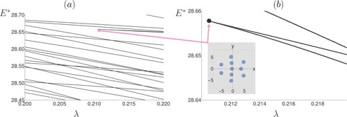
For larger values of N it remains possible to find and catalogue the stable equilibrium solutions using conjugate gradient methods. For example, in the case of N = 10 we find that for low values of λ less than 0.0273 there are two stable equilibrium solutions. At $\lambda =0.0273$ the stable solution with the higher energy becomes unstable at a bifurcation point and only one stable solution remains; see Figure 8. While such details can still be glimpsed for N = 10, with increasing N the number of unstable equilibrium solutions rapidly proliferates and the task of identifying solutions becomes nearly impossible. To give some idea of the large number of states involved even for N = 10, we have searched for all equilibrium solutions within a narrow range, as shown in Figure 9(a). Amongst the vast number of crossing lines it is possible to identify features such as blue sky bifurcations (see Figure 9(b)), similar to that seen for N = 5.

Figure 8. N = 10. Stable equilibrium solutions are shown in blue. For low values of λ there are two stable solutions, as shown in the inset. Also shown in the inset are some of the unstable equilibrium solutions (in black), it can be seen that one of the stable solutions becomes unstable at a bifurcation point (indicated by the large black dot).

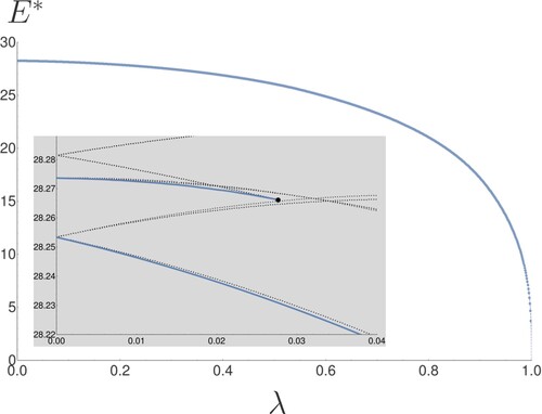
Figure 9. N = 10. (a) A narrow region of the bifurcation diagram (i.e. Figure 8) for N = 10, showing all the equilibrium solutions. (b) Close-up showing a blue sky bifurcation.

6. Conclusion

We have shown that an extraordinary variety of interesting (stable and unstable) equilibrium structures is found for the confined system of N ions. We have examined these in various limits and diagrammed their evolution in terms of the reduced energy and the anisotropy of the confining potential. Only for small N can the dense interior of this diagram be readily explored computationally (see Figures 2,3,4 and 5). We have tentatively explored some of the features of larger systems (see Figures 8 and 9) and intend to confront this problem in greater depth in future work. Included in such remaining challenges is the development of individual and multiple kinks in the zigzag structure of Figure 1(a).

All simulations presented here were for ions interacting via Coulomb forces. Based on published experimental and numerical studies we expect qualitatively similar results for ions interacting via a screened Coulomb (Yukawa) potential, although the details of the energy bifurcation diagrams will differ [24].

We have previously analysed the properties of simpler but broadly analogous systems, consisting of hard spheres (or disks), confined in a line by a transverse harmonic potential and compressed between two hard walls (in two dimensions) [25–29]. The insights gained from this, as regards bifurcation diagrams and Peierls–Nabarro potentials [30], are valuable in the present context. In those previous studies the key property was the instability of linear arrangements with respect to a lateral zigzag instability, when compressed, as is also found here.

While there are some similarities between the buckling of hard spheres and ions there are also many subtle differences. For example, in the case of the hard spheres unstable solutions were seen in the experiments, as they were stabilised by friction [29]. While unstable equilibrium states may not be readily accessible in the case of ions in experiment, they are nevertheless valuable in understanding the reason why the linear chain becomes unstable. This is clearly demonstrated in the case of N = 5 (see the second inset in Figure 5): the linear chain becomes unstable with decreasing anisotropy at a bifurcation point, beyond which the linear chain continues as an unstable solution while the zigzag arrangement now becomes the only stable solution.

In further work we have computed hundreds of arrangements for the large number of 50 ions [31]. The observed intricacy of the patterns makes them a worthwhile object of study in their own right, be it in the context of computer-generated art, or for use in psycho-physical studies of the perception of randomness and order.

Disclosure statement

No potential conflict of interest was reported by the author(s).

Additional information

Funding

AM acknowledges the support of the Supercomputing Wales project, which is part-funded by the European Regional Development Fund (ERDF) via the Welsh Government.

References

- S. Mavadia, J.F. Goodwin, G. Stutter, S. Bharadia, D.R. Crick, D.M. Segal, and R.C. Thompson, Control of the conformations of ion Coulomb crystals in a Penning trap, Nat. Commun. 4 (2013), pp. 1–7.
- R.C. Thompson, Ion Coulomb crystals, Contemp. Phys. 56 (2015), pp. 63–79.
- G. Birkl, S. Kassner, and H. Walther, Multiple-shell structures of laser-cooled 24mg+ ions in a quadrupole storage ring, Nature 357 (1992), pp. 310–313.
- L. Yan, W. Wan, L. Chen, F. Zhou, S. Gong, X. Tong, and M. Feng, Exploring structural phase transitions of ion crystals, Sci. Rep. 6 (2016), pp. 1–9.
- D.J. Wineland, J. Bergquist, W.M. Itano, J. Bollinger, and C. Manney, Atomic-Ion Coulomb Clusters in an Ion Trap, Phys. Rev. Lett. 59 (1987), pp. 2935–2938.
- D. Porras and J.I. Cirac, Effective quantum spin systems with trapped ions, Phys. Rev. Lett. 92 (2004), Article ID 207901.
- G. Piacente, I. Schweigert, J.J. Betouras, and F. Peeters, Generic properties of a quasi-one-dimensional classical Wigner crystal, Phys. Rev. B 69 (2004), Article ID 045324.
- S. Fishman, G. De Chiara, T. Calarco, and G. Morigi, Structural phase transitions in low-dimensional ion crystals, Phys. Rev. B 77 (2008), Article ID 064111.
- J. Schiffer, Phase transitions in anisotropically confined ionic crystals, Phys. Rev. Lett. 70 (1993), pp. 818–821.
- H. Landa, B. Reznik, J. Brox, M. Mielenz, and T. Schätz, Structure, dynamics and bifurcations of discrete solitons in trapped ion crystals, New. J. Phys. 15 (2013), Article ID 093003.
- V.M. Bedanov and F.M. Peeters, Ordering and phase transitions of charged particles in a classical finite two-dimensional system, Phys. Rev. B 49 (1994), pp. 2667–2676.
- F. Bolton and U. Rössler, Classical model of a Wigner crystal in a quantum dot, Superlattices. Microstruct. 13 (1993), pp. 139.
- O. Rancova, E. Anisimovas, and T. Varanavičius, Structural transitions in laterally compressed two-dimensional Coulomb clusters, Phys. Rev. E. 83 (2011), Article ID 036409.
- C.D. Bruzewicz, J. Chiaverini, R. McConnell, and J.M. Sage, Trapped-ion quantum computing: Progress and challenges, Appl. Phys. Rev. 6 (2019), Article ID 021314.
- H.L. Partner, R. Nigmatullin, T. Burgermeister, K. Pyka, J. Keller, A. Retzker, M.B. Plenio, and T.E. Mehlstäubler, Dynamics of topological defects in ion Coulomb crystals, New. J. Phys. 15 (2013), Article ID 103013.
- Wolfram player. Available at https://www.wolfram.com/player/.
- A. Radzvilavičius, O. Rancova, and E. Anisimovas, Dimensional transitions in small Yukawa clusters, Phys. Rev. E. 86 (2012), Article ID 016404.
- Figure 3. Available at https://www.wolframcloud.com/obj/527d1bd5-b4bf-4b47-b0af-59219891550a.
- Figure 3. Available at www.wolframcloud.com/obj/8db4e637-1979-48fa-8036-ca355d6bb7ef.
- Figure 4. Available at https://www.wolframcloud.com/obj/c8c78af4-fcdb-410a-98a8-d6a8ac2c64a2.
- See accompanying file ‘figure-5-interactive.nb’ to be opened using Wolfram player.
- R.C. HilbornChaos and Nonlinear Dynamics: An Introduction for Scientists and Engineers, 2nd ed., Oxford University Press, 2000.
- See accompanying file ‘Figure-6-and-7-interactive.nb’ to be opened using Wolfram player.
- T. Sheridan and K. Wells, Dimensional phase transitions in small yukawa clusters, Phys. Rev. E 81 (2010), Article ID 016404.
- J. Winkelmann, A. Mughal, D. Weaire, and S. Hutzler, Equilibrium configurations of hard spheres in a cylindrical harmonic potential, EPL (Europhys. Lett.) 127 (2019), Article ID 44002.
- D. Weaire, A. Irannezhad, A. Mughal, and S. Hutzler, A simple experimental system to illustrate the nonlinear properties of a linear chain under compression, Am. J. Phys. 88 (2020), pp. 347–352.
- S. Hutzler, A. Mughal, J. Ryan-Purcell, A. Irannezhad, and D. Weaire, Buckling of a linear chain of hard spheres in a harmonic confining potential: numerical and analytical results for low and high compression, Phys. Rev. E. 102 (2020), Article ID 022905.
- D. Weaire, A. Mughal, J. Ryan-Purcell, and S. Hutzler, Description of the buckling of a chain of hard spheres in terms of Jacobi functions, Physica D 433 (2022), Article ID 133177.
- A. Irannezhad, D. Weaire, A. Mughal, J. Ryan-Purcell, and S. Hutzler, Buckling of a tilted line of confined hard spheres, Philos. Mag. 102 (2022), pp. 2506–2524.
- A. Mughal, D. Weaire, and S. Hutzler, Peierls-Nabarro potential for a confined chain of hard spheres under compression, Europhys. Lett. 135 (2021), Article ID 26002.
- A. Mughal, S. Hutzler, and D. Weaire, Coulomb calligraphy, Forma (2022 – submitted).