A function improving tip loss correction of blade-element momentum theory for wind turbines

ABSTRACT

Tip loss correction is necessary for all aerodynamic computations based on the blade-element momentum theory (BEMT) that plays an essential role in wind turbine design. Glauert tip-loss correction, which is most widely used, assumes the rotor is lightly loaded and thus lose some accuracy for modern wind turbines that are highly loaded. In the present work, a new g-function involving the rotor’s thrust-coefficient is introduced, which connects the tip loss correction with the rotor’s load condition and reduces the error of the tip loss correction. Computational tests are performed on two rotors that are distinct in size and tip shape. The new g-function results in good consistency between the computed forces and the reference data, exhibiting excellent role in improving the accuracy of the BEMT computations. In general, the new g-function combines good effectiveness and applicability, and thus has great potential for engineering applications.

KEYWORDS:

• Wind turbine
• aerodynamics
• tip loss correction
• blade-element momentum theory

1. Introduction

The huge and growing installation of wind power capacity has greatly enhanced the interests of improving the accuracy of wind turbine design methods. The global new wind power capacity connected to power grids was 77.6 GW in 2022. It would be a miscalculation of 776 MW if the worldwide used methods had an inaccuracy of 1% in power prediction. The current averaged costs of onshore and offshore installations are about 1.3 and 2.8 million dollars per MW respectively, and the 1% (776 MW) worth about 1.0 billion dollars for onshore installations and 2.2 billion dollars for offshore installations.

The blade-element momentum theory (BEMT) (Elfering et al. 2023; Hansen 2000; van Kuik, Sørensen, and Okulov 2015) is the standard algorithm used in aerodynamic performance certification of commercial wind turbines. It plays an essential role in power/load prediction and blade shape design for wind and tidal turbines (Bai and Wang 2016; Escalera Mendoza, Griffith, and Jeong 2023; Jeong et al. 2024; Li et al. 2023). However, it has uncertainties of accuracy in multiple engineering models it employs (Fritz, Ferreira, and Boorsma 2022; Sayed et al. 2019; Wang et al. 2023). Tip loss correction is one necessary kind of the models. Researchers have pointed out that the most widely used tip loss correction, Glauert tip loss correction, generally leads to overestimation of the force contribution of the tip area of wind turbine blades (Branlard 2011; Schmitz and Maniaci 2017; Zhong et al. 2020), especially at high tip-speed ratio where the tip aerodynamic load can be overestimated by 5%–15% (Boatto et al. 2023). Such an overestimation of force, especially its tangential component that directly contributes torque and power, needs to be repaired to avoid miscalculation of wind power capacity. Therefore, the present study focuses on solving the inaccuracy of tip loss correction.

Tip loss occurs on any wing or blade with finite span moving in the air, although there are different understandings between the tip loss of a translational wing and that of a rotor. The tip loss of a translational wing is purely considered as a three-dimensional (3-D) effect due to its finite span (Smith and Ventikos 2021), while the tip loss of a rotor is conventionally considered as an effect of its finite number of blades (Okulov and Sørensen 2008). From a physical point of view (Li, Dong, and Cheng 2020; van Kuik et al. 2014), the tip loss of either a wing or a rotor is originated from the 3-D effect. The specific characteristic of a rotor’s tip loss lies in the fact that the 3-D effect of one blade can be reduced by the interference of the helical tip vortices generated by all blades of the rotor. Consequently, a rotor’s tip loss would be eliminated if its number of blades or tip speed ratio became infinite.

For predicting the aerodynamic performance of a practical rotor with finite number of blades, tip loss correction becomes essential in any methods including BEMT based on the two-dimensional (2-D) hypothesis. The BEMT links the aerodynamic performance of rotating 3-D blades with that of the 2-D airfoils forming the blades, based on the momentum theory and the 2-D blade-element assumption. This linkage allows the airfoils’ aerodynamic data to be applied to rotating blade-elements. However, it is not adequately valid in the blade tip and root regions where the flow has noticeable 3-D characteristics. The aerodynamic forces of these regions must be corrected by introducing a tip/root loss correction into BEMT. This kind of correction receives more attention at the tip than the root, as the tip region contributes much more torque and power than the root region. In practical applications, the root loss is corrected in a manner highly similar to the tip loss correction.

A tip loss correction of the BEMT usually consists of two parts. One is a tip loss factor, and the other is an approach of performing the correction with the tip loss factor. The first tip loss factor for a rotor is originated from the study of Prandtl (1921) on screw propellers. He proposed a function making Betz’s optimal circulation (Betz 1919) of a blade go to zero at the blade tip, which was later recognized as the first tip loss factor for practical rotors with finite number of blades. Glauert (1963) considered the physical meaning of the tip loss factor as the ratio between the azimuthally averaged induced velocity and the induced velocity at the blade position, and consequently made a modification to the Prandtl tip loss factor. Furthermore, he for the first time introduced how the tip loss factor can be used as a correction to the BEMT. Thus, it was Prandtl who derived the first tip loss factor and Glauert firstly proposed an approach of application, and the first tip loss correction can be seen as a common contribution of Prandtl and Glauert. Nowadays in wind turbine aerodynamics, the concepts of Prandtl tip loss correction and Glauert tip loss correction are not strictly distinguished.

It is worth noting three points about the Glauert tip loss factor (or the Prandtl tip loss factor): first, it was developed based on the ideal rotor of Betz that was defined as a rotor producing minimum energy loss; second, it is not an exact description but an approximate expression of the optimal circulation corresponding to Betz’s ideal rotor; furthermore, even Betz’s ideal rotor itself does not strictly valid from a practical standpoint. For the ideal rotor, Betz stated that the trailing vortices of the rotor blades form rigid vortex sheets moving with a constant velocity. However, the realistic vortices cannot strictly keep rigid in the near wake of the rotor, since the near wake contracts for a propeller and expands for a wind turbine. As Sørensen (2016) pointed out, the ideal rotor model of Betz contains an inconsistency since the helical pitch of a rigid vortex sheet cannot be the same in the rotor plane as in the wake. The basis of the Glauert tip loss factor is thus somewhat inconsistent with the facts. This inconsistency would be more serious if the rotor were operating in a state deviates from that of Betz’s ideal rotor. As pointed out by Schmitz and Maniaci (2017), Maniaci and Schmitz (2016), the Glauert tip loss factor is rooted from high-solidity and lightly loaded propellers, which results in a persistent over-prediction of the blade tip force for modern low-solidity and highly loaded wind turbines. That’s to say, the Glauert tip loss correction is suitable for lightly loaded rotors that are more consistent with Betz’s ideal rotor, while its applicability to modern highly loaded wind turbine rotors is somewhat questionable.

A lot of work has been made in the past few decades to improve the Glauert tip loss correction or establish new corrections. Wilson and Lissaman (1974) made a modification to Glauert tip loss correction, correcting not only the induced velocity but also the axial mass flux through the rotor plane. de Vries (1979) further modified the correction to correct both the axial and tangential mass flux. An additional factor was proposed by Shen, Mikkelsen, et al. (2005) to directly correct the force of blade-elements, as a supplement to Glauert tip loss correction. Shen’s factor was later showed also conducive to a better prediction of tip force in actuator line/Navier-Stokes (AL/NS) simulations (Shen, Sørensen, and Mikkelsen 2005; Wimshurst and willden 2017). Sørensen, Dag, and Ramos-Garía (2015) established a new correction called the de-camber correction describing the effect of the streamline bending caused by the non-uniform downwash flow around the bade tip. Wood, Okulov, and Bhattacharjee (2016), Wood (2018) applied the vortex theory to the blade-element analysis and derived three methods for direct calculation of tip loss. Zhong et al. (2020) proposed a new tip loss correction which involves two factors representing the 3-D effect and the rotational effect respectively.

The above studies to some extent repaired the accuracy of tip loss correction. However, the developed corrections are either much more complex than the Glauert tip loss correction or have not been tested on various wind turbines. The Glauert tip loss correction is still dominant in engineering applications owing to its ease of use and extensive validations, and there is no indication that it may be replaced. Therefore, it is significantly meaningful to further improve the tip load prediction based on the framework of the Glauert tip loss correction.

The fundamental shortcoming of the Glauert tip loss correction rooted from the light-load assumption. Such a disadvantage must be eliminated in order to make the correction consistent with the high-load fact of modern large wind turbines. The thrust coefficient is the indicator for determining whether a rotor is lightly or highly loaded. In the present work, a novel new g-function involving the rotor’s thrust coefficient is proposed and introduced into the Glauert tip loss factor, which connects the tip loss correction with the rotor’s load condition and thus fundamentally extends the range of good accuracy from light-load condition to both light and high load conditions. It will be shown in the following parts of this paper how the new g-function is established and to what extent it can improve the tip loss correction for wind turbines.

2. Introduction to g-functions

The Glauert tip loss factor is well known as (1) $F={\displaystyle \frac{2}{\pi }{\cos }^{-1}\left\{\exp \left[-{\displaystyle \frac{B\left(R-r\right)}{2\mathrm{rsin}\varphi }}\right]\right\}}$(1) where B is the number of blades, R is the rotor radius, r is the local radius, and $\varphi$ denotes the local inflow angle.

Shen, Mikkelsen, et al. (2005) for the first time introduced a g-function into the above expression, resulting in (2) $F_1={\displaystyle \frac{2}{\pi }{\cos }^{-1}\left\{\exp \left[-\mathrm{g}\left(\lambda \right){\displaystyle \frac{B\left(R-r\right)}{2\mathrm{rsin}\varphi }}\right]\right\}}$(2) in which their g-function is defined as (3) $\mathrm{g}\left(\lambda \right)=\exp \left[-c_1\left(\mathrm{B\lambda }-c_2\right)\right]$(3) where $\lambda$ is the tip speed ratio, and $c_1$ and $c_2$ are empirical constants.

Inspired by Shen’s work, Schmitz and Maniaci (2017), Maniaci and Schmitz (2016) defined another g-function, $\mathrm{g}\left(r\right)$, resulting in a modified Glauert tip loss factor that we here denoted as $F_{\mathrm{Sc}}$ (4) $F_{\mathrm{Sc}}={\displaystyle \frac{2}{\pi }{\cos }^{-1}\left\{\exp \left[-\mathrm{g}\left(r\right){\displaystyle \frac{B\left(R-r\right)}{2\mathrm{rsin}\varphi }}\right]\right\}}$(4) The $\mathrm{g}\left(r\right)$ function was defined as a combination of two segments shown in Figure 1, which can be described using the following algebraic expression: (5) $\mathrm{g}\left(r\right)=\{\begin{array}{cc}1& ,r/R\le 0.82\\ k\cdot r/R+b& ,0.82<r/R\le 1.0\end{array}$(5) where $k$ and $b$ are empirical constants.

Figure 1. Graph of the g-function proposed by Schmitz et al.

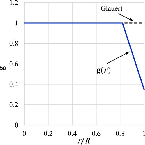
Schmitz et al. applied the tip loss factor with $\mathrm{g}\left(r\right)$ to the BEMT computations of the NREL UAE Phase VI rotor and the accuracy of the tip force prediction is improved. However, there are two imperfections of Schmitz’s g-function: first, there is a first-order parametric discontinuity at the junction of the two segments, which is inconsistent with the physical fact that the aerodynamic force on a blade composed of smooth surfaces should be smoothly distributed; second, the constants $k$ and $b$ need to be recalibrated as the blade operates at various pitch angles, indicating that such a g-function cannot be uniform even for a specific rotor.

3. New g-function

3.1. The role of load effect

The fundamental defect of the Glauert tip loss factor lies in assuming the rotor is lightly loaded (Sørensen 2016). Such an assumption means the rotor’s thrust coefficient $C_T$, which is defined as follows, is regarded as approximately equal to zero. (6) $C_T={\displaystyle \frac{T}{{\displaystyle \frac{1}{2}\rho V_0^{2}A}}}$(6) where $T$ is the thrust load of the rotor, $\rho$ is the air density, $V_0$ is the wind speed and $A$ denotes the rotor swept area.

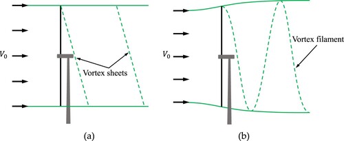
However, modern wind turbines are usually highly loaded (Schmitz and Maniaci 2017). The difference of the theoretical wake model of Glauert and a model closer to the real situation are demonstrated in Figure 2. The wake expansion is related to the rotor’s load situation, and the light load assumption adopted by Glauert’s model implies the wake expansion is ignored. The wake expansion has an effect on the development of the rotor’s tip vortices which determines the rotor’s tip loss. Therefore, the light-load assumption may lead to inaccurate evaluation of tip loss especially as the rotor is highly loaded.

Figure 2. The theoretical wake model of Glauert (a) and a model closer to the real situation (b).

According to the momentum theory, $C_T$ is related to the axial interference factor $a$ by $C_T=4a\left(1-a\right)$. For example, $C_T$ values 0.36, 0.64 and 0.89 as the rotor operates at $a$ = 0.1, 0.2 and 1/3, respectively. The Betz limit of maximum power coefficient is corresponding to a = 1/3, and thus theoretically a wind turbine should most frequently operate around a = 1/3. As shown in the above example, a = 1/3 leads to $C_T$ = 0.89 which is obviously much higher than zero. Therefore, the load effect should not be ignored for modern wind turbines, and thus $C_T$ should be included as a key parameter in the tip loss correction.

3.2. The expression of new g-function

In the present study, taking the rotor’s thrust load into account, a new g-function denoted by $\mathrm{g}\left(T\right)$ is proposed, resulting in a modified Glauert tip loss factor that we here denote as $F_T$, (7) $F_T={\displaystyle \frac{2}{\pi }{\cos }^{-1}\left\{\exp \left[-\mathrm{g}\left(T\right){\displaystyle \frac{B\left(R-r\right)}{2\mathrm{rsin}\varphi }}\right]\right\}}$(7)

The understandings about the role of load effect motivated us to establish the new g-function involving the thrust coefficient $C_T$ as a key parameter. We set the following principles for establishing the new g-function: (1) there is a dividing point of the blade span, denoted as r* here, the inboard of which keeps g = 1.0 while the outboard has g < 1.0; (2) the g-r curve holds first-order parametric continuity at any spanwise location including r = r*; (3) in the range of r > r*, g declines as r increases, and the decline becomes sharper with the increase of $C_T$. The first principle is learned from Schmitz’s g-function. The second principle makes the new g-function more consistent with the aerodynamic fact. The third principle makes the new g-function involve $C_T$ as a key parameter, which is an important innovation of the present work.

According to the above principles, the expression of the new g-function is eventually defined as (8) $\mathrm{g}\left(T\right)=\{\begin{array}{cc}1.0& ,r\le r^{\ast }\\ \cos \left({\displaystyle \frac{\pi }{2}{f}_T{\displaystyle \frac{r-r^{\ast }}{R-r^{\ast }}}}\right)& ,r>r^{\ast }\end{array}$(8) in which $f_T$ is determined by $C_T$ as (9) $f_T=\{\begin{array}{cc}m{C}_T^n& ,m{C}_T^n\le 1.0\\ 1.0& ,m{C}_T^n>1.0\end{array}$(9) where n denotes an empirical constant as the exponent of $C_T$, and m is another empirical constant making a linear scaling of $C_T^n$.

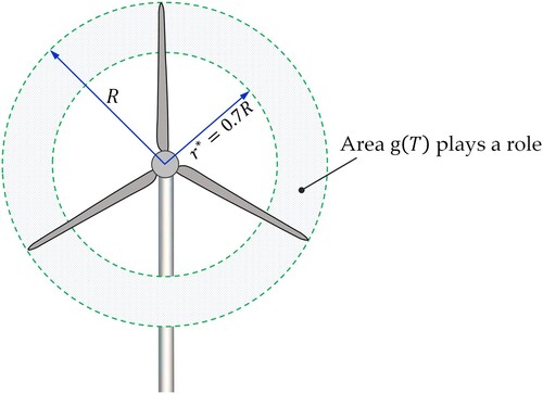
In the range of $r\le r^{\ast }$, $\mathrm{g}\left(T\right)$ = 1.0 and thus the $F_T$ defined in Equation (7) becomes identical to the $F$ defined in equation (1). That’s to say, the new g-function does not play a role in the above range. The r* is recommended to be set as 0.7R since this position is generally considered as the starting point of the blade tip region. As a result, the role of the new g-function is limited in the annular area shown in Figure 3.

Figure 3. The area where the new g-function plays a role.

3.3. The graph of new g-function

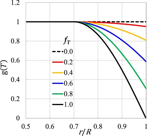
Figure 4 demonstrates the curves of the new g-function for various values of $f_T$ between 0 and 1.0. All curves coincide with the horizontal line of g = 1.0 in the range of $r\le 0.7R$, and then they diverge with different decline rates in $r>0.7R$. As $f_T$ = 0, the decline rate is zero and $\mathrm{g}\left(T\right)$ remains 1.0 in the entire blade span. As $f_T$ increases from 0 towards 1.0, the curves decline with rates positively correlated with the values of $f_T$. As $f_T$ = 1.0, the maximum decline rate is achieved, and the g-r curve ends with g = 0 at $r$= $R$.

Figure 4. Curves of the new g-function for various $f_T$ values.

4. Determining the constants m and n

4.1. Method of extracting g values from given force data

Adopting different values of the constants m and n leads to different results of the new g-function. Only by knowing some reference data of g values can we determine the constants. However, g values are not explicit in experimental measurements or computational fluid dynamics (CFD) simulations. We next try to extract g values from given force data of a blade.

The following equation can be derived from equation (7): (10) $\mathrm{g}\left(T\right)={\displaystyle \frac{2\mathrm{rsin}\varphi }{B\left(R-r\right)}\ln \left[1/\cos \left({\displaystyle \frac{\pi }{2}{F}_T}\right)\right]}$(10) It is valid regardless of the specific definitions of $\mathrm{g}\left(T\right)$ and $F_T$. For simplicity, we adopted the following general form of (11) $\mathrm{g}={\displaystyle \frac{2\mathrm{rsin}\varphi }{B\left(R-r\right)}\ln \left[1/\cos \left({\displaystyle \frac{\pi }{2}F}\right)\right]}$(11)

According to the above equation, g can be determined if $F$ and $\varphi$ have been known for a certain rotor. Therefore, we try to solve $F$ and $\varphi$ from the force data of a rotor.

The solving is made based on the BEMT theory, and the flowchart of the solving process for a blade element is shown in Figure 5. The main part of the solving process is an iterative procedure including 5 steps.

Figure 5. Procedure of solving the tip loss factor $F$ and the inflow angle $\varphi$.

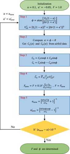
In step 1, the inflow angle $\varphi$ and the relative inflow velocity $V_{\mathrm{rel}}$ are computed from the input parameters of wind speed $V_0$, rotational speed $\mathrm{\Omega }$, local radius $r$, and the current values of axial interference factor $a$ and tangential interference factor $a^{\mathrm{\prime }}$.

In step 2, the angle of attack $\alpha$ is determined by the computed inflow angle $\varphi$ and the known local pitch angle $\theta$, and then the lift coefficient $C_l$ and drag coefficient $C_d$ are obtained from an interpolation of the airfoil data according to $\alpha$.

In step 3, the normal force coefficient $C_n$ and tangential force coefficient $C_t$ are obtained according to their relations with $C_l$ and $C_d$.

Step 4 is the core part of the iteration. The new value of $F$, denoted as $F_{\mathrm{new}}$, is obtained by (12) $F_{\mathrm{new}}=F+\mathrm{\Delta F}$(12) in which (13) $\mathrm{\Delta F}=0.1F\mathrm{\Delta }{C}_n,\mathrm{\Delta }{C}_n={\displaystyle \frac{{\tilde{C}}_n-C_n}{\left|{\tilde{C}}_n\right|+\left|C_n\right|},{\tilde{C}}_n={\tilde{F}}_n/{\displaystyle \frac{1}{2}\rho V_{\mathrm{rel}}^{2}c}}$(13)

In the above equations, the superscript ‘∼’ means that the value is determined by the given force data. The relation between $\mathrm{\Delta F}$ and $\mathrm{\Delta }{C}_n$ suggested in equation (13) is based on the fact that the computed $C_n$ is positively correlated with the value of $F$, i.e. $C_n\propto F$. The definition of $\mathrm{\Delta }{C}_n$ leads to $\left|\mathrm{\Delta }{C}_n\right|\le 1.0$, and further makes $\left|\mathrm{\Delta F}\right|=0.1F\left|\mathrm{\Delta }{C}_n\right|\le 0.1F$. That limits the variation of $F$ in each iteration to be less than 10% of its current value, enhancing the stability of the numerical iteration.

In step 5, new interference factors for the next iteration, $a_{\mathrm{new}}$ and $a_{\mathrm{new}}^{\mathrm{\prime }}$, are computed using the current resulting parameters including $F$.

$F$ and $\varphi$ are finally determined as the iteration is finished with $\left|a_{\mathrm{new}}-a\right|$<${10}^{-5}$. The value of g for the present blade element can then be determined using equation (11).

$F$ and $\varphi$ can also be determined if the parameters related to the normal force, i.e. ${\tilde{F}}_n$, ${\tilde{C}}_n$, $C_n$ and $\mathrm{\Delta }{C}_n$ are replaced by the tangential force related parameters of ${\tilde{F}}_t$, ${\tilde{C}}_t$, $C_t$ and $\mathrm{\Delta }{C}_t$, respectively. The results determined by the normal and tangential forces should be identical if the tip loss correction theory of Glauert is exactly the truth (however it is not exact) and the given force data are error free.

4.2. Determining m and n with extracted g values

The given force data for extracting g values can be measured in experiments or simulated by CFD. We chose CFD simulations since the force data in experiments such as the NREL UAE Phase VI (Hand, Simms, and Fingersh 2001) and the MEXICO (Boorsma and Schepers 2014; Snel, Schepers, and Montgomerie 2007) are only measured at few (usually only two) sections in the tip region (r/R > 0.7). The CFD simulated force data of the NREL UAE Phase VI rotor are chosen to extract g values. The simulation was made by the authors, the details of which can be found in (Zhong et al. 2018). The involving operating conditions are shown in Table 1, which covers regular tip speed ratios for wind turbines. The cases a, b, c and d lead to increasing values of the rotor’s thrust coefficient $C_T$ which are 0.48, 0.75, 0.85 and 0.91, respectively.

Table 1. Computational cases of the NREL UAE Phase VI rotor for extracting g values.

Case number	Wind speed (V0, m/s)	Rotating speed (Ω,rpm)	Tip speed ratio (λ)	Tip pitch angle (°)
a	7	72	5.42	3.0
b	7	90	6.78	−1.0
c	7	110	8.28	−1.0
d	7	130	9.78	−1.0

The extracted g values are plotted in Figure 6. There are two characteristics worth noting in the results of all the four cases. One is the downward trend of the g values as approaching the blade tip, which becomes more significant as the thrust coefficient increases. It confirms that the Glauert factor (corresponding to g≡1) does need to be corrected by introducing proper g values less than 1. The other is the difference between g values extracted from $C_n$ and those extracted from $C_t$. It implies that we cannot obtain the accurate normal and tangential forces simultaneously by applying identical g values. It further indicates that the framework of the Glauert correction cannot ensure both accurate normal and tangential forces at the same time no matter what the tip loss factor $F$ is taken.

Figure 6. The g values extracted from $C_n$ and $C_t$, and the corresponding g-functions.

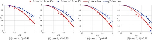
Different g values will be given by the new g-function (equations 8 and 9) as $m$ and $n$ take different values. After some attempts, their values were determined to be ($m$ = 0.95, $n$ = 0.2) and ($m$ = 0.8, $n$ = 0.3) for fitting the g values extracted from $C_n$ and $C_t$, respectively. We refer to the g-function with ($m$ = 0.95, $n$ = 0.2) as the g1-function and the other with ($m$ = 0.8, $n$ = 0.3) as the g2-function. The curves of the g1 and g2 functions are plotted in Figure 6, exhibiting good fittings of the extracted g values.

It is a question that whether the g1 or g2 function should be adopted in the tip loss factor. We recommend prioritising the use of the g2-function because it is determined by the extracted g values corresponding to the tangential force which is essential to the rotor’s power output. The g1-function gives lower g values and consequently leads to an excessive downward correction of the tangential force, although it is more suitable for predicting the normal force. As a result, we take the g2-function as the finally accepted g-function in the next computations in the present study. If researchers require the best prediction of both the normal and tangential forces, the g2 and g1 functions can be independently used to successively solve the tangential and normal forces. In this way, the g2-function is firstly adopted, and the tangential force is taken when the solving is converged. It is then replaced with the g1-function, and the normal force is taken when the solving is converged again.

5. Application of new g-function

5.1. Steps of BEMT computations employing the new g-function

The application of the new g-function is easy for any existing BEMT codes. The present computations are performed using a code based on the classic BEMT (Hansen 2000) which gives equations (14)–(19).

For each blade element, the inflow angle is calculated by (14) $\varphi ={\tan }^{-1}{\displaystyle \frac{\left(1-a\right)V_0}{\left(1+a^{\mathrm{\prime }}\right)\mathrm{\Omega }r}}$(14) and the angle of attack is determined by (15) $\alpha =\varphi -\theta$(15) where $\theta$ is the local pitch angle.

The normal force coefficient $C_n$ and tangential force coefficient $C_t$ of the blade element are related to the airfoil’s lift coefficient $C_l$ and drag coefficient $C_d$ by (16) $C_n=C_l\cos \varphi +C_d\sin \varphi$(16) (17) $C_t=C_l\sin \varphi -C_d\cos \varphi$(17)

The axial and tangential interference factors are then determined by (18) $a={\left({\displaystyle \frac{4F{\sin }^2\varphi }{\sigma C_n}+1}\right)}^{-1}$(18) (19) $a^{\mathrm{\prime }}={\left({\displaystyle \frac{4\mathrm{Fsin}\mathrm{\varphi cos}\varphi }{\sigma C_t}-1}\right)}^{-1}$(19) where $\sigma =\mathrm{Bc}/2\mathrm{\pi r}$ (c is the chord length of the blade element).

The steps listed in Table 2 is adopted as the procedure of the BEMT computation employing the new g-function. There is one problem in the step 3.3 that the rotor’s thrust coefficient $C_T$ that is necessary in equation (9) has not been available before all blade elements have been computed. There are two ways to obtain an approximate value of $C_T$: one is making a pre-computation with the standard Glauert tip loss correction for all blade elements, and calculating $C_T$ using equation (6) with the thrust and area of the whole rotor; the other is determining $C_T$ using equation (6) with the cumulative thrust and swept area of the elements that have been computed. The former way gives more accurate $C_T$ of the rotor while involves an additional pre-computation. The latter way avoids pre-computation but leads to a $C_T$ of part of the rotor rather than its entirety. We finally chosen the latter way to make the following computations because: (1) an additional pre-computation may reduce the acceptance of the new g-function in practical applications; (2) the $C_T$ values given by the two ways become closer to each other as approaching the blade tip.

Table 2. Steps of BEMT computation employing the new g-function.

Step number	Description
1	Discretising the blade into elements that are sequentially indexed from root to tip by i (i = 1,2, … ,N).
2	Initialising with i = 1, $a$ = 0.1 and $a^{\mathrm{\prime }}$ = −0.05.
3	Performing steps 3.1∼3.6 for the ith blade element.
3.1	Calculating $\varphi$ and $\alpha$ by equations (14) and (15).
3.2	Getting $C_l$ and $C_d$ from airfoil data and calculating $C_n$ and $C_t$ by equations (16) and (17).
3.3	Calculating $\mathrm{g}\left(T\right)$ by equations (8) and (9), and the tip loss factor $F_T$ by equation (7).
3.4	Updating $a$ and $a^{\mathrm{\prime }}$ by equations (18) and (19) with $F=F_T$.
3.5	Making a correction to high values of $a$, e.g. using Spera’s correction (Hansen 2000).
3.6	Going to step 3.1 until the computational residuals of $a$ and $a^{\mathrm{\prime }}$ are lower than expectation.
4	Saving $a$, $a^{\mathrm{\prime }}$, $C_n$, $C_t$, etc., and calculating normal force $F_n$ and tangential force $F_t$ for the current blade element.
5	If i < N, letting i = i + 1 and going to step 3.
6	Calculating concerned parameters of the rotor, e.g. the thrust, torque and power.

5.2. Computational cases

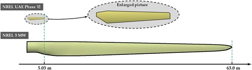
BEMT computations with and without the new g-function (‘without the new g-function’ means using the standard Glauert tip loss factor, i.e. equation (1)) are applied to the aerodynamic performance prediction of two rotors, the NREL UAE Phase VI rotor (2001) and the NREL 5MW rotor (Jonkman, Butterfield, and Musial 2009). The two rotors are distinct in size and blade-tip shape, and their blades consist of different airfoils. The NREL UAE Phase VI rotor has a radius of 5.03 m and blades with blunt tip, while the NREL 5MW rotor has a radius of 63.0 m and blades with sharp tip. The airfoil S809 is used as the profile of all blade sections of the NREL UAE Phase VI blade (except the root part), while several airfoils are used to the NREL 5MW blade and the airfoil NACA64_A17 is used in the tip region. The distinct size and blade-tip shape of the two rotors are demonstrated in Figure 7.

Figure 7. Sketch of distinct size and blade-tip shape of NREL UAE Phase VI and NREL 5MW blades.

All computational cases are listed in Table 3, in which the cases 1∼5 are for the NREL UAE Phase VI rotor, and cases 6∼9 are for the NREL 5MW rotor. The cases for each rotor are numbered in ascending order of their operating tip speed ratio.

Table 3. List of computational cases.

Rotor name	Case number	Wind speed (V0, m/s)	Rotating speed (Ω,rpm)	Tip speed ratio (λ)	Tip pitch angle (°)
NREL UAE Phase VI	1	7.0	72	5.42	3.0
	2	6.0	72	6.32	3.0
	3	7.0	90	6.77	−1.0
	4	7.0	110	8.28	−1.0
	5	7.0	130	9.78	−1.0
NREL 5MW	6	15.0	12.06	5.30	10.45
	7	11.4	12.06	6.98	0
	8	8.0	9.22	7.60	0
	9	6.0	7.49	8.24	0

The cases 1 and 2 are identical to the corresponding test conditions of the NREL UAE Phase VI experiments, and thus experimental reference data are available for them. There is a limitation for the adoption of the computational conditions: no flow separation occurs around the blade tip. The Glauert tip loss correction becomes unreliable as flow separation occurs (Zhong et al. 2020), which is another topic beyond the scope of the present study. As a result, except the above two, other usually referenced test conditions of the experimental rotor are not involved in the present computations since they encounter flow separation more or less.

The cases 3∼5 are artificially set by the authors in order to extend the tip speed ratio of the NREL UAE Phase VI rotor to higher values (Higher tip speed ratio leads to higher $C_T$ as the blade pitch remain unchanged).

The cases 6∼9 are several conditions taken from the design operating curve of the NREL 5MW rotor, among which the case 7 is the rated operating condition of the rotor.

5.3. Results of NREL UAE phase VI rotor

The computed normal and tangential force coefficients ($C_n$ and $C_t$) along a blade of the NREL UAE Phase VI rotor are plotted in Figure 8. Experimental data are available for cases 1 and 2 as a reference, and CFD data are presented for all the cases 1∼5.

Figure 8. Normal and tangential force coefficients along a blade of the NREL UAE Phase VI rotor.

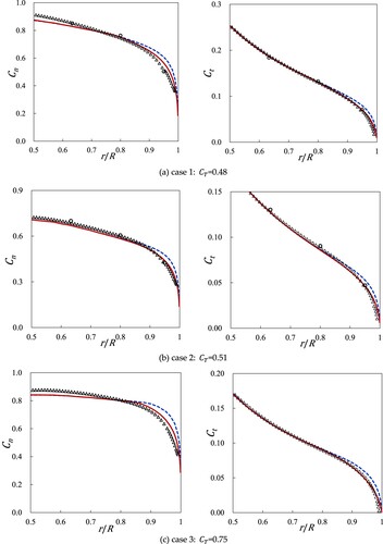
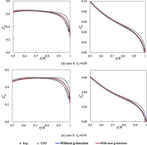
As shown in Figure 8(a)–(e), the forces computed without the new g-function are generally higher than the reference data. In the computations with the new g-function, for all the 5 cases, the normal force coefficient $C_n$ is predicted much closer to the reference data, and the tangential force coefficient $C_t$ becomes in good agreement with the reference data. The benefit of applying the new g-function, which can be evaluated by the size of the gap between the two computed curves, becomes more significant with the increasing of the rotor’s thrust coefficient from case 1 to case 5.

Such a result clearly exhibits that: (1) the blade’s tip force is generally over-predicted in computations employing the standard Glauert tip loss factor; (2) The over-prediction can be well repaired by applying the new g-function; (3) the benefit brought by the new g-function becomes greater as the rotor is more highly loaded.

5.4. Results of NREL 5MW rotor

The normal and tangential forces ($F_n$ and $F_t$) on a blade of the NREL 5MW rotor are plotted in Figure 9, showing the force curves of the BEMT computations with and without the g-function and the reference data from CFD.

Figure 9. Normal and tangential forces on a blade of the NREL 5MW rotor.

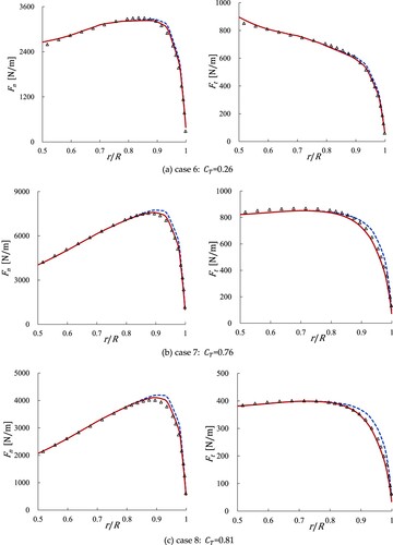
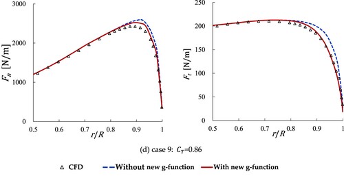
As shown in Figure 9(a)–(d), before the new g-function is applied, all the computed force curves are higher than the reference data in the tip region, which becomes more serious as $C_T$ increases. The relative errors of the computed forces at a typical tip section of r/R = 0.95 are listed in Table 4. From case 6 ($C_T$ = 0.26) to case 9 ($C_T$ = 0.86), the relative error of $F_n$ increases from 6.6% to 11.3% and that of $F_t$ increases from 6.2% to 17.9%.

Table 4. Errors of the computations without new g-function (at r/R = 0.95 of the NREL 5MW blade).

Case number	${\mathit{C}}_{\mathit{T}}$	Relative error of ${\mathit{F}}_{\mathit{n}}$	Relative error of ${\mathit{F}}_{\mathit{t}}$
8	0.26	6.6%	6.2%
9	0.76	7.7%	9.4%
10	0.81	9.4%	13.1%
11	0.86	11.3%	17.9%

Applying the new g-function to these cases leads to $F_n$ curves notably closer to the reference data and $F_t$ curves highly consistent with the reference data. Such a result demonstrates the great advantage of the new g-function in improving the BEMT computations for such a large rotor.

6. Conclusions

A new g-function improving the tip loss correction of BEMT has been proposed and validated in aerodynamic computations of wind turbines. The thrust coefficient $C_T$ is taken as the key argument representing the rotor’s load effect in the new g-function. That establishes an analytical expression relating the tip loss with the load condition of the rotor, and thus repairs the fundamental defect of the Glauert tip loss correction in which all rotors are assumed lightly loaded.

The study shows several superior characteristics of the new g-function including: (1) Its application can greatly improve the accuracy of the tip load prediction for rotors in different size and tip shape, which has been well demonstrated on the NREL UAE Phase VI rotor and the NREL 5MW rotor. (2) Its expression can keep uniform for various rotors and operating conditions, making it easy to be used in engineering practices. (3) Its role is negligible as the rotor is lightly loaded ($C_T$≈0) and becomes more significant as the load increases, and thus can be seen as seamlessly extending the range of good accuracy for the Glauert tip loss correction.

In general, the new g-function exhibits good effectiveness and applicability. Considering the high-load character of modern large wind turbines, we believe that the new g-function is necessary and has great potential to be widely used in aerodynamic performance computations for wind turbine design. It provides more accurate tip load especially the tangential force that is essential to the rotor’s power output. The new g-function paves a feasible path for greatly improving the tip loss correction of BEMT for wind turbines, and it is very helpful if researchers test the new g-function on more wind turbines and improve it if necessary.

Disclosure statement

No potential conflict of interest was reported by the author(s).

Data availability statement

The data that support the findings of this study are available from the corresponding author, W. Zhong, upon reasonable request.

Additional information

Funding

This work was supported by National Key Research and Development Program of China [grant number 2022YFE0207000].

References

- Bai, C., and W. Wang. 2016. “Review of Computational and Experimental Approaches to Analysis of Aerodynamic Performance in Horizontal-Axis Wind Turbines (HAWTs).” Renewable and Sustainable Energy Reviews 63: 506–519. https://doi.org/10.1016/j.rser.2016.05.078.
- Betz, A. 1919. “Schraubenpropeller Mit Geringstem Energieverlust – Mit Einem Zusatz Von l. Prandtl.” Göttinger Klassiker der Strömungsmechanik Bd 3: 68–88. (in German).
- Boatto, U., P. A. Bonnet, F. Avallone, et al. 2023. “Assessment of Blade Element Momentum Theory-Based Engineering Models for Wind Turbine Rotors Under Uniform Steady Inflow.” Renewable Energy 214: 307–317. https://doi.org/10.1016/j.renene.2023.04.050.
- Boorsma, K., and J. G. Schepers. 2014. New MEXICO Experiment: Preliminary Overview with Initial Validation. ECN-E-14-048.
- Branlard, E. 2011. Wind Turbine Tip-Loss Corrections. Master’s Thesis, Technical University of Denmark.
- de Vries, O. 1979. Fluid Dynamic Aspects of Wind Energy Conversion. AGARD Report AG-243, chap. 4, 1–50. Amsterdam: National Aerospace Laboratory.
- Elfering, K., R. Metoyer, P. Chatterjee, et al. 2023. “Blade Element Momentum Theory for a Skewed Coaxial Turbine.” Ocean Engineering 269: 113555.
- Escalera Mendoza, A. S., D. T. Griffith, and M. Jeong. 2023. “Aero-Structural Rapid Screening of New Design Concepts for Offshore Wind Turbines.” Renewable Energy 219: 119519. https://doi.org/10.1016/j.renene.2023.119519.
- Fritz, E. K., C. Ferreira, and K. Boorsma. 2022. “An Efficient Blade Sweep Correction Model for Blade Element Momentum Theory.” Wind Energy 25 (12): 1977–1994.
- Glauert, H. 1963. “Airplane Propellers.” In Aerodynamic Theory, edited by W. F. Durand, 169–360. New York: Dover.
- Hand, M. M., D. A. Simms, and L. J. Fingersh. 2001. Unsteady Aerodynamics Experiment Phase VI: Wind Tunnel Test Configurations and Available Data Campaigns. Golden: National Renewable Energy Laboratory, NREL/TP-500-29955.
- Hansen, M. O. L. 2000. Aerodynamics of Wind Turbines. London, UK: James & James (Science Publishers) Ltd.
- Jeong, M., E. Loth, C. Qin, et al. 2024. “Aerodynamic Rotor Design for a 25 MW Offshore Downwind Turbine.” Applied Energy 353: 122035.
- Jonkman, J., S. Butterfield, and W. Musial. 2009. Definition of a 5-MW Reference Wind Turbine for Offshore System Development. Golden: National Renewable Energy Laboratory, NREL/TP-500-38060.
- Li, C., H. Dong, and B. Cheng. 2020. “Tip Vortices Formation and Evolution of Rotating Wings at Low Reynolds Numbers.” Physics of Fluids 32: 021905. https://doi.org/10.1063/1.5134689.
- Li, Z., G. Li, L. Du, et al. 2023. “Optimal Design of Horizontal Axis Tidal Current Turbine Blade.” Ocean Engineering 271: 113666. https://doi.org/10.1016/j.oceaneng.2023.113666.
- Maniaci, D. C., and S. Schmitz. 2016. “Extended Glauert Tip Correction to Include Vortex Rollup Effects.” Journal of Physics: Conference Series 753: 022051. https://doi.org/10.1088/1742-6596/753/2/022051.
- Okulov, V. L., and J. N. Sørensen. 2008. “Refined Betz Limit for Rotors with a Finite Number of Blades.” Wind Energy 11: 415–426. https://doi.org/10.1002/we.274.
- Prandtl, L. 1921. Applications of Modern Hydrodynamics to Aeronautics. NACA report No. 116. Washington, DC: NationaI Advisory Committee for Aeronautics.
- Sayed, M., L. Klein, T. H. Lutz, et al. 2019. “The Impact of the Aerodynamic Model Fidelity on the Aeroelastic Response of a Multi-Megawatt Wind Turbine.” Renewable Energy 140: 304–318.
- Schmitz, S., and D. C. Maniaci. 2017. “Methodology to Determine a Tip-Loss Factor for Highly Loaded Wind Turbines.” AIAA Journal 55: 341–351.
- Shen, W. Z., R. Mikkelsen, J. N. Sørensen, et al. 2005. “Tip Loss Corrections for Wind Turbine Computations.” Wind Energy 8: 457–475.
- Shen, W. Z., J. N. Sørensen, and R. Mikkelsen. 2005. “Tip Loss Correction for Actuator/Navier-Stokes Computations.” Journal of Solar Energy Engineering 127: 209–213.
- Smith, T. A., and Y. Ventikos. 2021. “Wing-Tip Vortex Dynamics at Moderate Reynolds Numbers.” Physics of Fluids 33: 035111. https://doi.org/10.1063/5.0039492.
- Snel, H., J. G. Schepers, and B. Montgomerie. 2007. “The MEXICO Project (Model Experiments in Controlled Conditions): The Database and First Results of Data Processing and Interpretation.” Journal of Physics: Conference Series 75: 012014.
- Sørensen, J. N. 2016. General Momentum Theory for Horizontal Axis Wind Turbines. Springer. 123–132. https://doi.org/10.1007/978-3-319-22114-4_8
- Sørensen, J. N., K. O. Dag, and N. Ramos-Garía. 2015. “A New Tip Correction Based on the Decambering Approach.” Journal of Physics: Conference Series 524: 012097.
- van Kuik, G. A. M., D. Micallef, I. Herraez, et al. 2014. “The Role of Conservative Forces in Rotor Aerodynamics.” Journal of Fluid Mechanics 750: 284–315. https://doi.org/10.1017/jfm.2014.256.
- van Kuik, G. A. M., J. N. Sørensen, and V. L. Okulov. 2015. “Rotor Theories by Professor Joukowsky: Momentum Theories.” Progress in Aerospace Sciences 73: 1–18.
- Wang, T., W. Zhong, Y. Qian, et al. 2023. Wind Turbine Aerodynamic Performance Calculation. Science Press and Springer. https://doi.org/10.1007/978-981-99-3509-3
- Wilson, R. E., and P. B. S. Lissaman. 1974. Applied Aerodynamics of Wind Power Machines. Oregon State University Report NSF/RA/N-74113.
- Wimshurst, A., and R. H. J. willden. 2017. “Analysis of a Tip Correction Factor for Horizontal Axis Turbines.” Wind Energy 20: 1515–1528. https://doi.org/10.1002/we.2106.
- Wood, D. H. 2018. “Application of Extended Vortex Theory for Blade Element Analysis of Horizontal-Axis Wind Turbines.” Renewable Energy 121: 188–194. https://doi.org/10.1016/j.renene.2017.12.085.
- Wood, D. H., V. L. Okulov, and D. Bhattacharjee. 2016. “Direct Calculation of Wind Turbine Tip Loss.” Renewable Energy 95: 269–276. https://doi.org/10.1016/j.renene.2016.04.017.
- Zhong, W., W. Z. Shen, T. Wang, et al. 2020. “A Tip Loss Correction Model for Wind Turbine Aerodynamic Performance Prediction.” Renewable Energy 147: 223–238. https://doi.org/10.1016/j.renene.2019.08.125.
- Zhong, W., H. Tang, T. Wang, et al. 2018. “Accurate RANS Simulation of Wind Turbine Stall by Turbulence Coefficient Calibration.” Applied Sciences 8: 1444.