Test-retest evaluation of a notched-noise test using consumer-grade mobile audio equipment

Abstract

Objective

The aim of this study was to investigate whether consumer-grade mobile audio equipment can be reliably used as a platform for the notched-noise test, including when the test is conducted outside the laboratory.

Design

Two studies were conducted: Study 1 was a notched-noise masking experiment with three different setups: in a psychoacoustic test booth with a standard laboratory PC; in a psychoacoustic test booth with a mobile device; and in a quiet office room with a mobile device. Study 2 employed the same task as Study 1, but compared circumaural headphones to insert earphones.

Study sample

Nine and ten young, normal-hearing participants completed studies 1 and 2, respectively.

Results

The test-retest accuracy of the notched-noise test on the mobile implementation did not differ from that for the laboratory setup. A possible effect of the earphone design was identified in Study 1, which was corroborated by Study 2, where test-retest variability was smallest when comparing results from experiments conducted using identical acoustic transducers.

Conclusions

Results and test-retest repeatability comparable to standard laboratory settings for the notched-noise test can be obtained with mobile equipment outside the laboratory.

Keywords:

• Notched-noise test
• telemedicine
• test-retest reliability

1. Introduction

Within the field of psychoacoustics, many experimental procedures are very time-consuming and some require training to familiarise the participants with the task and stabilise their performance before the data collection. Personal mobile devices show a large potential for aiding in psychoacoustic experiments, since implementing experiments as standalone mobile applications can allow participants to familiarise themselves with the task (e.g. at home) in advance. Mobile applications can also enable collection of longitudinal data with repeated measures without the need to visit the research site at each timepoint. Thus, personal mobile devices offer an appealing alternative to laboratory experiments (Brungart et al. 2018; Gallun et al. 2018; Swanepoel et al. 2019; van Zyl, Swanepoel, and Myburgh 2018). However, it is not known how well current psychoacoustic methods translate to mobile equipment and acoustically less controlled environments. So far, attention has been mainly directed at automated mobile versions of traditional audiometry, where the calibration of presentation levels and the level of environmental noise play a critical role. Despite suboptimal acoustic conditions and consumer-grade audio equipment at home, direct comparisons between audiometry conducted at a clinic by professional personnel and self-administered audiometry have shown no statistically significant differences in threshold estimates (Derin et al. 2016; Masalski and Kręcicki 2013; Whitton et al. 2016), although care must be taken when setting up the equipment (Barczik and Serpanos 2018; Corry, Sanders, and Searchfield 2017). Additionally, negative effects of background noise can be addressed to some extent with advanced signal processing approaches, such as active noise cancellation (Bromwich et al. 2008; Clark et al. 2017).

Greater tolerance of background noise can be expected for suprathreshold auditory tests—such as the notched-noise test (Glasberg and Moore 1990; Patterson 1976; Weber 1977)—due to higher signal presentation levels (and thus higher signal–to–background-noise-ratios). The notched-noise test determines detection thresholds for a pure-tone signal presented simultaneously with a broadband noise masker. The masker has a spectral notch centred at the signal frequency, and varying the spectral distance from the signal frequency to the lower and upper notch edges leads to changes in the detection thresholds. The changes of the thresholds can be explained by the concept of auditory filters, i.e. the frequency selectivity of the auditory system. Specifically, the power-spectrum model of masking predicts that the farther away the masker edges are from the signal, the less masker energy falls within the auditory filter centred at the signal’s frequency, thus reducing the signal threshold. Expressing the threshold as a function of notch width results in a curve from which the shape of the underlying auditory filter can be derived (Glasberg and Moore 1990). Degraded frequency selectivity of the auditory system has been found to be related to difficulties in understanding speech in a noisy background, even when the auditory thresholds are normal (Badri, Siegel, and Wright 2011; King and Stephens 1992; Strelcyk and Dau 2009), and therefore information about auditory filter shapes can complement standard audiological measures.

The notched noise test can be time-consuming, and due to the limited time available during a visit to an audiology clinic, additional auditory tests beyond the audiogram are often not feasible (Stone, Glasberg, and Moore 1992). It has been possible to shorten the time needed for conducting a frequency selectivity test (Rens Leeuw & Dreschler, 1994; Schlittenlacher, Turner, and Moore 2020; Sek et al. 2005; Shen, Kern, and Richards 2019; Shen, Sivakumar, and Richards 2014; Shen and Richards 2013), but the cost of including more experimental tests into the clinical assessment may still be too high. Therefore, automated mobile tests, which can be completed independently by the patient at home, can be used for additional audiological testing, providing the clinician with additional information on the patient’s hearing abilities.

The main focus of the current work was to determine whether there are any differences in the outcomes of a notched-noise test between a standard laboratory setup and a mobile platform. The same experimental procedure was conducted in a listening booth with laboratory equipment and a mobile phone to investigate possible hardware-related issues. In addition, the mobile device was tested in a regular office setting, in order to identify possible problems related to the various acoustic and non-acoustic effects of less acoustically controlled surroundings. After identifying a possible influence of earphone type on the results, a follow-up study was conducted where circumaural headphones were compared to insert earphones using the standard laboratory setup.

2. Methods

2.1. Study design

Study 1 compared the results from a standard laboratory setup to those obtained using a mobile phone. Study 2 compared the results from circumaural headphones to those from insert earphones, both collected using the standard laboratory setup.

All participants provided informed consent and all experiments were approved by the Science-Ethics Committee for the Capital Region of Denmark (reference H-16036391).

2.2. Hardware platforms

The two hardware platforms compared in the current study were a standard personal computer equipped for psychoacoustic research (referred to as PC), and an Apple iPhone 8 mobile phone (Phone).

On the PC, stimuli were generated with Matlab, D/A-converted by an external Fireface UCX soundcard, and amplified by a Sound Performance Lab Phonitor mini headphone amplifier. In Study 1, sounds were presented via Sennheiser HD-650 circumaural headphones. In Study 2, condition HD650 used Sennheiser HD-650 headphones, and condition ER2 used Etymotic ER-2 insert earphones.

On the Phone, stimuli were generated with the iOS vDSP library, included in the Accelerate framework, and presented via Apple EarPod earphones connected to the phone’s Lightning port. The mode of the AVAudioSession object used for playback of the stimuli was set to measurement in order to avoid any sound processing by the operating system.

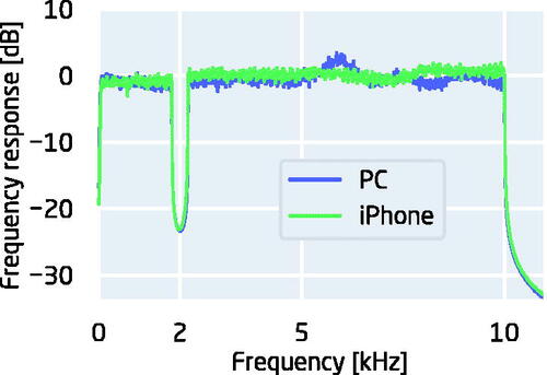
On both systems, a 44.1-kHz sampling rate was used. The frequency responses of the two systems were recorded using a B&K head and torso simulator (HATS, type 4128-C) with an artificial pinna and ear canal (DZ-9769) and a 2-cc coupler. The frequency response of each system was compensated by an inverse filter applied to the digital signal prior to the presentation. Spectra of example notched-noise stimuli, presented through the two systems after compensation are shown in Figure 1.

Figure 1. Two spectra of a noise band (0.01–10 kHz) with a spectral notch of ±0.2 kHz around 2 kHz, presented via the two different playback systems after compensating for differences in frequency responses by inverse filtering.

2.2.1. Study 1

Nine young, normal-hearing participants (7 male, 2 female) took part in Study 1.

The main interest of Study 1 was to evaluate whether the hardware platform or the environment had any effect on the results of a notched-noise experiment. Therefore, the following three conditions were included in the study: 1) PC in booth, 2) Phone in booth, and 3) Phone in room, where PC and Phone refer to the hardware platforms (Section 2.2), and booth and room refer to a double-walled acoustically treated listening booth, and a quiet office room, respectively. The level of background noise, expressed as A-weighted continuous equivalent sound pressure level $L_{\mathit{Aeq},10s}$ was 17.9 dB SPL in booth and 24.7 dB SPL in room. The Phone in room condition was repeated on another day to get an estimate of the test-retest variability for the same equipment and environment, and, prior to the actual experiment, all participants completed one PC in booth training block. Thus, in total all participants completed one training block and four experimental blocks.

2.2.2. Study 2

Ten young, normal-hearing participants (5 male, 5 female) took part in Study 2. With the exception of one participant, none of the participants had taken part in Study 1.

The main goal of Study 2 was to clarify whether some results of Study 1 could have been caused by the differences in the acoustic coupling of the earphones used in the PC and Phone conditions. Two conditions were included in Study 2: 1) PC with circumaural headphones, and 2) PC with insert earphones. We refer to these conditions as HD650 and ER2, respectively. The equipment is described in more detail in Section 2.2. Both conditions were repeated on a second day, in order to get an estimate of the test-retest variability for both earphone types for comparison with the results of Study 1. Prior to the actual experiment, all participants completed one training block with circumaural headphones. Thus, all participants completed one training block and four experimental blocks.

2.3. Notched-noise test

Detection thresholds for a 2-kHz tone, presented simultaneously with a broadband noise masker, were determined using a two-alternative forced-choice (2-AFC) paradigm. The masker was a white noise band with a frequency range from 0.1 to 10 kHz, with a symmetric notch around the signal frequency $f_S=$ 2 kHz. The masker spectrum had a notch between $f_S-\Delta f$ and $f_S+\Delta f.$ Following common practice in notched-noise experiments, the notch width is expressed in terms of the normalised value of frequency with respect to the signal frequency: $\Delta =\frac{\Delta f}{f_S}.$ In the current study, the total notch width corresponds to $2\Delta ,$ since the notch extends by $\Delta f$ both upwards and downwards in frequency relative to the signal frequency (Glasberg and Moore 1990; Moore and Glasberg 1987; Patterson 1976; Rosen and Baker 1994; Weber 1977). The spectral level of the masker was held constant at 30 dB SPL/Hz. The noise was generated via an inverse Fourier transform, where the frequency components had equal amplitude and uniformly distributed random phase for the frequencies in the two passbands, and zero amplitude for the frequencies within the notch and outside the masker frequency range.

The stimuli consisted of either the masker alone (non-signal interval) or the masker and the signal simultaneously (signal interval), in random order. The task of the 2-AFC trial was to indicate the signal interval. Visual feedback (correct/incorrect) was provided after each trial. The length of the stimuli was 300 ms, and the inter-stimulus interval was 400 ms. Sounds were presented monaurally to the left ear for most participants. For two participants in Study 2 the right ear was chosen instead, due to the presence of earwax or discomfort caused by the insert earphone in the left ear.

2.4. Grid tracking method

Traditionally, detection thresholds are determined based on individual experimental runs for each masker notch width of interest, using for example a transformed up-down method (Levitt 1971) with a fixed notch width, and varying only the target level. However, in this approach, each experimental run usually starts with the signal level well above the detection threshold. When this procedure is repeated for many notch widths, a considerable proportion of trials are conducted using signal levels far away from the threshold.

To shorten the time needed for estimating detection thresholds at multiple notch widths, the grid method of Fereczkowski (2015) was used. This aims to increase the proportion of trials with signal levels close to the threshold. The grid method estimates the full threshold curve during one experimental run by alternating between adjusting the notch width g and the signal level $L_{\mathit{sig}}$ (Figure 2). When $L_{\mathit{sig}}$ is adjusted, Δ is kept fixed until the detection threshold $L_{\mathit{sig}}^{\mathit{th}}(\Delta )$ has been determined. Then, $L_{\mathit{sig}}$ is fixed at the threshold value and Δ is adjusted until the detection threshold for Δ at that $L_{\mathit{sig}}$ is found. This process is continued until a predefined maximum notch width or minimum presentation level is reached.

Figure 2. Illustration of one run of the grid method. The track starts with a moderately high signal level at zero notch width. Level is decreased until the signal detection threshold ($L_{\mathit{sig}}^{\mathit{th}}(\Delta ),$ shown as a grey line) is reached, after which the notch is increased until there is again a correct response.

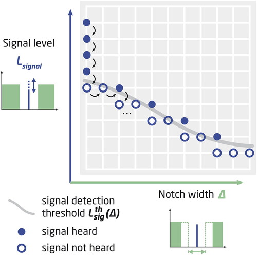
Just as in a transformed up-down method, different tracking rules can be implemented, such as 3-down–1-right (“right” referring to increasing notch width Δ, see Figure 2), which corresponds to the traditional 3-down-1-up rule, and the choice of parameters determines the point along the psychometric function (e.g. the 79.4% detection threshold for a 3-down–1-up track).

In the current study, the threshold at zero notch width was first determined with a 3-down–1-up staircase procedure, with four reversals using a 6-dB step size, followed by six reversals using a 3-dB step size. The threshold at zero notch width was calculated as the average signal level at the last six reversals. This threshold is referred to as the tone–in–noise-threshold. Then, the run continued with a 3-down–1-right grid procedure from the sixth reversal of the 3-down-1-up track. The run was terminated when either the maximum notch width of 0.5 or the minimum signal level of 30 dB SPL was reached. The minimum level was chosen to further shorten the time needed for testing, allowing more conditions to be investigated.

A single experimental block consisted of three repeated runs. A two-parameter rounded-exponential roex(p, r) filter model (Patterson et al. 1982) was fitted to the thresholds obtained in each run, and the resulting p and r parameters were averaged over each experimental block. The roex(p, r) filter shape is of the form: $$W\left(g\right)=\left(1-r\right)\left(1+\mathit{pg}\right)e^{-\mathit{pg}}+r,$$ where g is the deviation from filter centre frequency divided by the centre frequency.

3. Results and discussion

3.1. Study 1

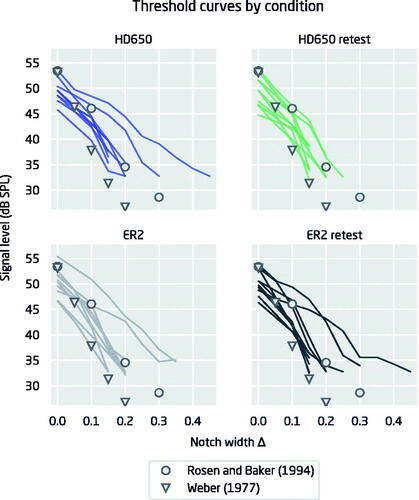
Figure 3 shows the threshold curves for each participant. By visual inspection, it is clear that the curves are very similar in all four cases. For comparison, each panel shows the data from Rosen and Baker (1994) and Weber (1977), for the same masker type, i.e. symmetric notch and 30 dB SPL/Hz spectral level. Up to notch widths of about 0.2 the slopes of the curves collected here seem similar to those from the literature, and in particular from Rosen and Baker (1994), as will be shown later.

Figure 3. Detection thresholds as a function of notch width for Study 1. Thin lines show the individual threshold curves. The round and triangular symbols are the same in all figures and show data from Rosen and Baker (1994) and Weber (1977), respectively.

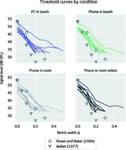
The thresholds obtained here for Δ = 0 are slightly below those from previous studies, and at larger notch widths the curves from the current study appear to flatten out due to the fact that in the current study the lower limit for the signal level was 30 dB SPL. While the reason for the differences in threshold curve shapes between the current study and earlier results is not clear, it is possible that feedback given during the experiments played a role. Whereas Rosen and Baker (1994) did not report whether feedback was given, in our study feedback was given after each answer. This can have the effect of lowering detection thresholds at Δ = 0, as found by Lukaszewski and Elliott (1962), who reported that auditory thresholds were on average 3.4 dB lower when feedback was given, compared to no feedback. Looking at the tone-in-noise thresholds in the current study, the difference to thresholds in Rosen and Baker (1994) is between −2.9 dB and −4.3 dB, for Phone in room retest and Phone in room conditions respectively, consistent with the finding of Lukaszewski and Elliot (1962). In a later study by Baker and Rosen (2006) with identical methodology, it was explicitly stated that feedback was used, but the masked thresholds at 2 kHz were very similar to the thresholds from the earlier study (Rosen and Baker 1994). Thus, it remains unclear whether providing feedback could explain the differences between the current study and earlier results. It should also be noted that both Weber (1977) and Rosen and Baker (1994) only had three participants in their studies. In the current study, a total of 18 participants took part in the listening experiments and in each condition the individual tone-in-noise thresholds were spread across approximately a 6-9 dB range. Expressed as standard deviations, the variability of threshold estimates for Δ = 0 was between 1.9 dB (PC in booth) and 2.0 dB (Phone in room retest). This is in line with Moore (1987), who reported a standard deviation of 2.0 dB for a notch width of 0.0. Given that the individual thresholds span such a wide range, it is possible that the differences between our study and those of Weber (1977) and Rosen and Baker (1994) reflect individual differences.

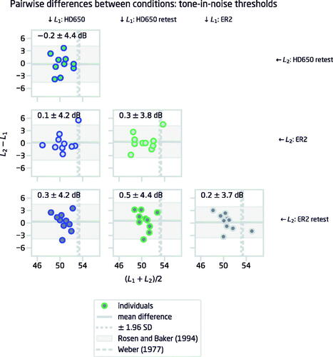
To investigate the differences between platforms and environments more systematically, the four experimental cases were compared in a pairwise manner with a Bland-Altman plot (Bland and Altman 1986), which is a method for assessing the agreement between two measures. Figure 4 shows the pairwise Bland-Altman plots for the tone-in-noise-thresholds. The largest mean difference between two conditions was 1.4 dB between the Phone in room and the Phone in room retest. The 95% limits of agreement (±1.96 × standard deviation) indicate the estimated range within which 95% of the individual test-retest differences are expected to lie. The widest limits of agreement (±4.6 dB) were between the Phone in booth and the Phone in room conditions.

Figure 4. Pairwise Bland–Altman plots visualising test–retest repeatability for tone–in–noise-thresholds (threshold at zero notch) between two conditions in Study 1. The horizontal line shows the average difference in thresholds between two conditions, and the shaded area illustrates the 95% limits of agreement (mean ±1.96 SD) between the two conditions. The vertical grey dashed lines show the tone–in–noise-thresholds from Rosen and Baker (1994) and Weber (1977).

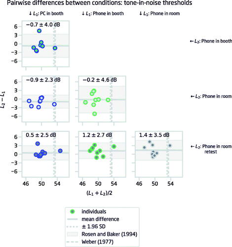
There are no clear patterns in the data, and in fact the test-retest accuracy is within expected limits for all conditions, as was verified by a Monte-Carlo simulation (1000 rounds) of the tone-in-noise-threshold determination. Simulations were run using the same experimental parameters as in the current study and reference values for the estimators from Schlauch and Rose (1990). Assuming the threshold estimate to be a normally-distributed variable $X\sim N(\mu ,{\sigma }^2),$ the simulated estimate of the standard deviation of a single threshold estimate was found to be 2 dB. Using this estimate, the distribution of the tone–in–noise-thresholds was calculated as the average over three repeated runs: $$\overline{X}=\frac{1}{3}\sum _{i=1}^3{X}_i=\sum _{i=1}^3\frac{1}{3}{X}_i\hspace{0.17em}\sim \hspace{0.17em}N\left(\sum _{i=1}^3\frac{1}{3}\mu ,\sum _{i=1}^3{\left(\frac{1}{3}\sigma \right)}^2\right)=N\left(\mu ,\hspace{0.17em}\frac{3}{9}{\sigma }^2\right)$$ and so, the variance of the averaged tone-in-noise-threshold is expected to be ${\overline{\sigma }}^2=\frac{3}{9}·{\left(2\mathrm{dB}\right)}^2=\frac{4}{3}{\mathrm{dB}}^2.$ For two conditions a and b, the difference in thresholds is expected to be also a normally distributed variable: $X_{\mathit{diff}}={\overline{X}}_a-{\overline{X}}_b\sim N\left(0,2{\overline{\sigma }}^2\right)=N\left(0,\frac{8}{3}{\mathrm{dB}}^2\right).$ If a sample ($n=9,$ the number of participants in Study 1) is drawn from this distribution, the 95% confidence interval for the limits of agreement would be 2.2 − 6.1 dB. This follows from the fact that the limits of agreement correspond to $1.96·\sigma ,$ and the confidence interval for $\sigma$ can be derived from the ${\chi }^2$ distribution. Thus, it is expected that with the current experimental design, the observed spread is not limited by the equipment or the environment, as in all cases the limits of agreement are smaller than those suggested by the simulations; the largest interval for the 95% limits of agreement for tone-in-noise threshold test-retest variability is for Phone in booth vs Phone in room, where the limits spread ±4.6 dB from the average. This is within the aforementioned confidence interval for the estimate.

The obtained thresholds were then used to fit a roex(p, r) auditory filter model (see Table 1 for model parameter mean values and Figure 5 for parameter p test-retest repeatability). Here, the results were more mixed. The absolute values of p were slightly lower than those predicted at 2 kHz by the equations in Glasberg and Moore (1990; p_l = 32.1, p_u = 33.6), but similar to the values from Rosen and Baker (1994; p_l = 25.5, p_u = 26.7). The p values are also close to those reported at 2 kHz by Moore (1987; p = 26.3), although they used a masker spectrum level of 45 dB SPL, where the higher level is likely to result in wider auditory filters, and lower p values. The k parameter values are lower than in Rosen and Baker (1994; k = −2.9 dB) and Moore (1987; k = −0.7 dB), which also reflects the lower thresholds at Δ = 0.

Figure 5. Pairwise Bland–Altman plots visualising test–retest repeatability for the p parameter of the roex filter in Study 1. The horizontal line shows the average difference in p, and the shaded area illustrates the 95% limits of agreement (mean ± 1.96 SD) between the two conditions.

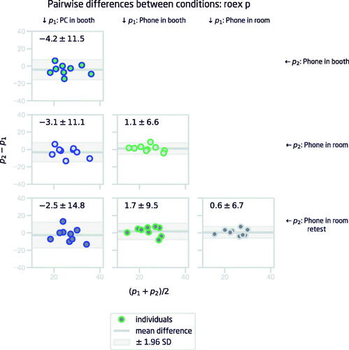
Table 1. The mean (standard deviation) of the p parameter and the corresponding equivalent rectangular bandwidth (erb) of the roex filter for each condition of Study 1.

Condition	p	r/dB	k/dB	erb/Hz
PC in booth	27.4 (6.9)	−72 (33)	−4.6 (2.6)	309 (78)
Phone in booth	23.2 (6.1)	−106 (50)	−4.8 (2.4)	366 (99)
Phone in room	24.3 (5.0)	−90 (40)	−5.6 (1.8)	343 (77)
Phone in room retest	24.9 (5.1)	−98 (50)	−4.1 (2.0)	336 (85)

Overall, the test-retest repeatability of the p parameter is relatively good across all conditions. Shen, Kern, and Richards (2019) assessed the reliability of a Bayesian adaptive procedure for estimating roex model parameters, and found the 95% limits of agreement for p to be −0.4 ± 18.7, which is slightly higher than PC in booth vs Phone in room retest (−2.5 ± 14.8) in the current study. However, the phone conditions show even better agreement with each other than with the PC in booth. The source of this discrepancy between PC and phone conditions is not clear from the data in Study 1. If the poorer agreement was due to differences in, for example, the frequency responses of the two systems, the test-retest differences should show a systematic error. Since the average difference is close to zero, it appears that the differences are driven by individual variability. One factor that could play a role is the difference in headphones. For the PC, the headphones were circumaural, whereas the EarPods are in-ear earbuds. Thus, although both systems were calibrated with the same HATS setup, it is plausible that individual differences in the coupling between headphones/earbud and the ear affected the spectral content and thereby the shape of the threshold curve. For example, changes in the ear canal resonance caused by the partial insertion of the EarPod might explain the observed differences. This hypothesis was tested in Study 2.

3.2. Study 2

Figure 6 shows the individual threshold curves for the two repeated conditions investigated in Study 2. The results were very similar to those of Study 1 and there were again no dramatic differences between conditions. Just as in Study 1, the thresholds for Δ = 0 were lower than those found by Rosen and Baker (1994); the offset at zero notch width was −2.6 dB in the ER2 retest and −3.1 dB in the HD650 retest.

Figure 6. Detection thresholds as a function of notch width for Study 2. The thin lines show the individual threshold curves. The round and triangular symbols are the same in all figures and show data from Rosen and Baker (1994) and Weber (1977), respectively.

The Bland-Altman plots for the tone-in-noise thresholds in Figure 7 show that there were no systematic differences between different types of headphones, and that the individual variability was within the expected range for the experimental paradigm (see Section 3.1).

Figure 7. Pairwise Bland–Altman plots visualising test–retest repeatability for tone–in–noise-thresholds (threshold at zero notch) between the two conditions in Study 2. The horizontal line shows the average difference in thresholds between two conditions, and the shaded area illustrates the 95% limits of agreement (mean ±1.96 SD) between the two conditions. The vertical grey dashed lines show the tone–in–noise-thresholds from Rosen and Baker (1994) and Weber (1977).

The roex model fits gave similar results to those found in Study 1 (Table 2); p values were similar to those from Rosen and Baker (1994) and lower than those from Glasberg and Moore (1990), and k values were slightly lower than in Rosen and Baker (1994) apart from ER2, where k = −2.8 was very close to Rosen and Baker’s value of k = −2.9. Figure 8 shows the Bland-Altman plots for the roex p parameter. Comparing the results to those in Figure 5, the same patterns can be seen here: the test-retest variability is smallest when using insert earphones (ER2 vs ER2 retest; Phone in room vs Phone in room retest in Study 1), and greatest when comparing results from two different types of headphones (e.g. HD650 retest vs ER2 retest; PC in booth vs Phone in booth in Study 1). The within-participant test-retest variability indicates that it is indeed an individual effect that cancels out at a group level, since there is no systematic bias in the p parameter values. These findings provide some support for the hypothesis that the acoustic characteristics of the coupling between headphone/earbud and the ear can have an effect on the thresholds. However, the test-retest repeatability is also very good for the circumaural headphones (HD650 vs HD650 retest), so it does not seem to be the case that insert earphones would provide considerably more accurate results than circumaural headphones, but that when comparing notched noise test results performed at different timepoints, it is important to keep experimental equipment as similar as possible.

Figure 8. Pairwise Bland–Altman plots visualising test–retest repeatability for the p parameter of the roex filter in Study 2. Horizontal line shows the average difference in p, and the shaded area illustrates the 95% limits of agreement (mean ± 1.96 SD) between the two conditions.

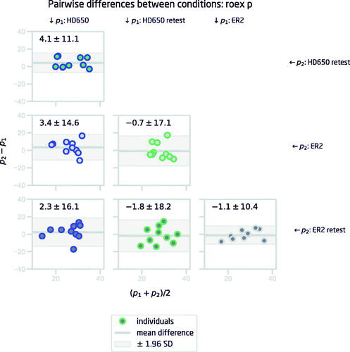
Table 2. The mean (standard deviation) of the p parameter and the corresponding equivalent rectangular bandwidth (erb) of the roex filter for each condition of Study 2.

condition	p	r/dB	k/dB	erb/Hz
HD650	24.6 (6.9)	−124 (33)	−4.9 (1.8)	351 (108)
HD650 retest	28.7 (6.5)	−102 (31)	−3.8 (3.1)	291 (65)
ER2	28.0 (5.4)	−129 (40)	−2.8 (3.0)	294 (53)
ER2 retest	27.0 (7.7)	−111 (52)	−3.9 (2.9)	327 (125)

It is remarkable that the consumer-grade earphones used with the phone gave similar test-retest repeatability to the research-grade insert earphones. Of course, this does not indicate that the electroacoustic characteristics are similar, only that the characteristics as well as earphone placement/coupling are stable across multiple sessions and over days. This was an unexpected finding, since it was assumed that results obtained with the phone would show larger variability due to imprecise positioning of the earphone. Based on the results of Study 1, it seems that participants were able to position the earphone in a consistent manner, despite receiving no specific instructions about earphone placement. They were however asked to take off and reinsert the earphone after each experimental run; this was not done for the HD-650s or the ER2s. The stability of results obtained using consumer-grade earphones in a self-administered experiment is a promising finding for future at-home studies.

4. Conclusions

Conducting the notched-noise test on a mobile phone and outside a sound-insulated listening booth did not influence the detection thresholds in the notched-noise test. Tone-in-noise-threshold estimation was not affected by differences in equipment or surroundings, as there were no differences in test-retest results between conditions. For the estimates of auditory frequency resolution, the larger spread (but no systematic bias) of test-retest differences between PC and phone was probably caused by different earphone designs, which was confirmed by a follow-up study comparing circumaural headphones and insert earphones.

The current results demonstrate that the notched-noise test can be performed with a mobile device and consumer-grade earphones, and in acoustically less controlled environments, without introducing bias or loss of test-retest accuracy in the results. Thus, there is potential for a mobile version of the notched-noise test, which can be self-administered, for example, as part of a field study.

Disclosure statement

No potential conflict of interest was reported by the author(s).

References

- Badri, R., J. H. Siegel, and B. A. Wright. 2011. “Auditory Filter Shapes And High-Frequency Hearing In Adults Who Have Impaired Speech In Noise Performance Despite Clinically Normal Audiograms.” The Journal of the Acoustical Society of America 129 (2): 852–863. doi:10.1121/1.3523476.
- Baker, R. J., and S. Rosen. 2006. “Auditory Filter Nonlinearity Across Frequency Using Simultaneous Notched-Noise Masking.” The Journal of the Acoustical Society of America 119 (1): 454–462. doi:10.1121/1.2139100.
- Barczik, J., and Y. C. Serpanos. 2018. “Accuracy of Smartphone Self-Hearing Test Applications Across Frequencies And Earphone Styles In Adults.” American Journal of Audiology 27 (4): 570–580. doi:10.1044/2018_AJA-17-0070.
- Bland, M. J., and D. G. Altman. 1986. “Statistical Methods for Assessing Agreement Between Two Methods Of Clinical Measurement.” The Lancet 327 (8476): 307–310. doi:10.1016/S0140-6736(86)90837-8.
- Bromwich, M. A., V. Parsa, N. Lanthier, J. Yoo, and L. S. Parnes. 2008. “Active Noise Reduction Audiometry: A Prospective Analysis of A New Approach To Noise Management in Audiometric Testing.” The Laryngoscope 118 (1): 104–109. doi:10.1097/MLG.0b013e31815743ac.
- Brungart, D., J. Schurman, D. Konrad-Martin, K. Watts, J. Buckey, O. Clavier, P. G. Jacobs, S. Gordon, and M. F. Dille. 2018. “Using Tablet-Based Technology to Deliver Time-Efficient Ototoxicity Monitoring.” International Journal of Audiology 57 (sup4): S78–S86. doi:10.1080/14992027.2017.1370138.
- Clark, J. G., M. Brady, B. R. Earl, P. M. Scheifele, L. Snyder, and S. D. Clark. 2017. “Use of Noise Cancellation Earphones in Out-Of-Booth Audiometric Evaluations.” International Journal of Audiology 56 (12): 989–996. doi:10.1080/14992027.2017.1362118.
- Corry, M., M. Sanders, and G. D. Searchfield. 2017. “The Accuracy And Reliability Of An App-Based Audiometer Using Consumer Headphones: Pure Tone Audiometry In A Normal Hearing Group.” International Journal of Audiology 56 (9): 706–710. doi:10.1080/14992027.2017.1321791.
- Derin, S., O. H. Cam, H. Beydilli, E. Acar, S. S. Elicora, and M. Sahan. 2016. “Initial Assessment of Hearing Loss Using A Mobile Application For Audiological Evaluation.” The Journal of Laryngology and Otology 130 (3): 248–251. doi:10.1017/S0022215116000062.
- Fereczkowski, M. 2015. “Time-Efficient Behavioral Estimates Of Cochlear Compression.”. PhD Thesis., Technical University of Denmark.
- Gallun, F. J., A. Seitz, D. A. Eddins, M. R. Molis, T. Stavropoulos, K. M. Jakien, S. D. Kampel et al. 2018. “Development and Validation of Portable Automated Rapid Testing (PART) measures for auditory research.” Proceedings of meetings on acoustics Acoustical Society of America 33(1). doi:10.1121/2.0000878.
- Glasberg, B. R., and B. C. J. Moore. 1990. “Derivation of auditory filter shapes from notched-noise data.” Hearing Research 47 (1-2): 103–138. doi:10.1080/20022727.2018.1430976.
- King, K., and D. Stephens. 1992. “Auditory and psychological factors in ‘auditory disability with normal hearing.” Scandinavian Audiology 21 (2): 109–114. doi:10.3109/01050399209045990.
- Levitt, H. 1971. “Transformed Up‐Down Methods in Psychoacoustics.” The Journal of the Acoustical Society of America 49 (2B): 467–477. doi:10.1121/1.1912375.
- Lukaszewski, J. S., and D. N. Elliott. 1962. “Auditory Threshold as a Function of Forced‐Choice Technique, Feedback, and Motivation.” The Journal of the Acoustical Society of America 34 (2): 223–228. doi:10.1121/1.1909173.
- Masalski, M., and T. Kręcicki. 2013. “Self-Test Web-Based Pure-Tone Audiometry: Validity Evaluation and Measurement Error Analysis.” Journal of Medical Internet Research 15 (4): e71–12. doi:10.2196/jmir.2222.
- Moore, B. C. J. 1987. “Distribution Of Auditory-Filter Bandwidths at 2 kHz in Young Normal Listeners.” The Journal of the Acoustical Society of America 81 (5): 1633–1635. doi:10.1121/1.394518.
- Moore, B. C. J., and B. R. Glasberg. 1987. “Formulae Describing Frequency Selectivity as a Function Of Frequency and Level, and Their Use in Calculating Excitation Patterns.” Hearing Research 28 (2-3): 209–225. doi:10.1016/0378-5955(87)90050-5.
- Patterson, R. D. 1976. “Auditory Filter Shapes Derived with Noise Stimuli.” The Journal of the Acoustical Society of America 59 (3): 640–654. doi:10.1121/1.380914.
- Patterson, R. D., I. Nimmo-Smith, D. L. Weber, and R. Milroy. 1982. “The Deterioration Of Hearing With Age: Frequency Selectivity, The Critical Ratio, The Audiogram, And Speech Threshold.” The Journal of the Acoustical Society of America 72 (6): 1788–1803. doi:10.1121/1.388652.
- Leeuw, A. R., and W. A. Dreschler. 1994. “Frequency-Resolution Measurements With Notched Noises For Clinical Purposes.” Ear and Hearing 15 (3): 240–255. doi:10.1097/00003446-199406000-00005.
- Rosen, S., and R. J. Baker. 1994. “Characterising Auditory Filter Nonlinearity.” Hearing Research 73 (2): 231–243. doi:10.1016/0378-5955(94)90239-9
- Schlauch, R. S., and R. M. Rose. 1990. “Two‐, Three‐, And Four‐Interval Forced‐Choice Staircase Procedures: Estimator Bias and Efficiency.” The Journal of the Acoustical Society of America 88 (2): 732–740. doi:10.1121/1.399776.
- Schlittenlacher, J., R. E. Turner, and B. C. J. Moore. 2020. “Application of Bayesian Active Learning to the Estimation of Auditory Filter Shapes Using the Notched-Noise Method.” Trends in Hearing 24:2331216520952992. doi:10.1177/2331216520952992.
- Sek, A., J. Alcántara, B. C. J. Moore, K. Kluk, and A. Wicher. 2005. “Development of a Fast Method for Determining Psychophysical Tuning Curves.” International Journal of Audiology 44 (7): 408–420. doi:10.1080/14992020500060800.
- Shen, Y., A. B. Kern, and V. M. Richards. 2019. “Toward routine Assessments of Auditory filter Shape.” Journal of Speech, Language, and Hearing Research : JSLHR 62 (2): 442–455. doi:10.1044/2018_JSLHR-H-18-0092.
- Shen, Y., and V. M. Richards. 2013. “Bayesian Adaptive Estimation Of The Auditory Filter.” The Journal of the Acoustical Society of America 134 (2): 1134–1145. doi:10.1121/1.4812856.
- Shen, Y., R. Sivakumar, and V. M. Richards. 2014. “Rapid Estimation of High-Parameter Auditory-Filter Shapes.” The Journal of the Acoustical Society of America 136 (4): 1857–1868. doi:10.1121/1.4894785.
- Stone, M. A., B. R. Glasberg, and B. C. J. Moore 1992. “Simplified Measurement of Auditory Filter Shapes Using The Notched-Noise Method.” British Journal of Audiology 26 (6): 329–334. doi:10.3109/03005369209076655.
- Strelcyk, O., and T. Dau. 2009. “Relations Between Frequency Selectivity, Temporal Fine-Structure Processing, And Speech Reception in Impaired Hearing.” The Journal of the Acoustical Society of America 125 (5): 3328–3345. doi:10.1121/1.3097469.
- Swanepoel, D. W., K. C. De Sousa, C. Smits, and D. R. Moore. 2019. “Mobile Applications to Detect Hearing Impairment: Opportunities and Challenges.” Bulletin of the World Health Organization 97 (10): 717–718. doi:10.2471/BLT.18.227728.
- van Zyl, M., D. W. Swanepoel, and H. C. Myburgh. 2018. “Modernising Speech Audiometry: Using a Smartphone Application to Test Word Recognition.” International Journal of Audiology 57 (8): 561–569. doi:10.1080/14992027.2018.1463465.
- Weber, D. L. 1977. “Growth of Masking and the Auditory Filter.” The Journal of the Acoustical Society of America 62 (2): 424–429. doi:10.1121/1.381542.
- Whitton, J. P., K. E. Hancock, J. M. Shannon, and D. B. Polley. 2016. “Validation of a Self-Administered Audiometry Application: An Equivalence Study.” The Laryngoscope 126 (10): 2382–2388. doi:10.1002/lary.25988.