Intraday Bitcoin price shocks: when bad news is good news

ABSTRACT

Since the formulation of the Efficient Market Hypothesis, countless studies have been developed that try to either prove or refute it. Event studies, analysing the impact of different events on asset prices, are one of the most important research fields but there is a lack of evidence on cryptocurrencies. For that reason, we analyse the existence of over- and under- reaction effects on Bitcoin after hourly price shocks defined by filter sizes. We also do this using three alternative approaches. Our results show clear evidence of overreaction after negative shocks. We also observe that these overreactions tend to be greater as more hours pass after the event, with those that occur between 6 and 24 hours after the event being especially important. These results have important economic implications because they show that investors would be able to develop a profitable trading strategy simply by focusing on investing after negative shocks.

KEYWORDS:

• Bitcoin
• price shocks
• average cumulative returns
• overreaction
• underreaction

1. Introduction

The studies of Fama (1965, 1970) and Samuelson (1965), who consider that stock prices reflect all available information and there is no possibility of generating statistically significant profits from any asset using any strategy or procedure, are the basis of the Efficient Market Hypothesis (EMH), They are also the basis for countless empirical works that try to prove or refute this, looking for inefficiencies or anomalies, from the most varied points of view, see Titan (2015) and Singh, Babshetti, and Shivaprasad (2022) for a systematic review of the empirical literature.

Event studies are a field of empirical evidence that enables an observer to assess the impact of a particular event on a firm’s stock price, as stated by Bodie, Kane, and Marcus (2018). This methodology has become a generally accepted tool to measure the economic impact of a wide range of events such as price shocks that can be defined in several ways. In this context, event studies become even more important as a tool for understanding the reaction of the financial markets to these extreme price shocks. This is because they can provide an accurate prediction of the subsequent behaviour of prices, which can be contrary to the previous movement (overreaction) or a continuation of the trend (underreaction or momentum), thus contradicting the efficient market hypothesis.

Atkins and Dyl (1990) and Bremer and Sweeney (1991) were the first to analyse stock market behaviour following a price shock, identifying the largest price change over a rolling window and for a filter size, respectively. Their studies were followed by others such as those of Cox and Peterson (1994), Fabozzi, Ma, Chittenden, and Pace (1995), Fung, Mok, and Lam (2000), Benou and Richie (2003), Grant, Wolf, and Yu (2005), Ising, Schiereck, Simpson, and Thomas (2006), Himmelmann, Schiereck, Simpson, and Zschoche (2012), Miralles-Marcelo, Miralles-Quirós, and Miralles-Quirós (2014) and Kolaric, Kiesel, and Schiereck (2016), among others.

However, the analysis of price behaviour after an event is not limited to large price changes. There are other studies which analyse prices after breaking support or resistance levels, see Brock, Lakonishok, and LeBaron (1992) and Bogards, Czudaj, and Van Hoang (2021) among others, and those which employ Bollinger Bands (see Plastun, Sibande, Gupta, & Wohar, 2021). Finally, Piccoli et al. (2017a, 2017b) analyse the effect of extreme price movements by considering the Value-at-Risk, VaR, to define them.

The arrival of new assets such as cryptocurrencies, mainly characterised by high volatility involving stratospheric rises followed by sudden crashes, especially at the intraday level, has increased interest in predicting price behaviour.

There are some interesting studies focused on cryptocurrency markets, such as Troster, Tiwari, Shahbaz, and Macedo (2019), Zhang, Chan, and Nadarajah (2019), Bogards and Czudaj (2020), (2021), Gerritsen, Bouri, Ramezanifar, and Roubaud (2020), Resta, Pagnottoni, and De Giuli (2020), Bouri, Lau, Saeed, Wang, and Zhao (2021), Hudson and Urquhart (2021), Naeem, Bouri, Peng, Shahzad, and Vo (2021), Diaconaşu, Mehdian, and Stoica (2022), Shahzad, Bouri, Ahmad, and Naeem (2022), Wang, Bouri, and Ma (2022), and Wen, Bouri, Xu, and Zhao (2022), which show heterogeneous results. However, the previous mentioned link between price shocks and over- or under- reactions has not been sufficiently developed in the empirical evidence because, to the best of our knowledge, only the works of Caporale and Plastun (2019, 2020) and Kellner and Maltritz (2022) belong to this research field.

This lack of evidence, together with the fact that there remain questions about whether cryptocurrency markets behave in an efficient manner, has led us to improve the previous empirical evidence in various ways. Initially, we analyse the existence of over- and under- reaction effects on Bitcoin after hourly price shocks defined by filter sizes. We follow the original approach of Bremer and Sweeney (1991) that, to the best of our knowledge, has not been applied to any cryptocurrencies. Secondly, we also employ three additional alternative approaches where price shocks are defined by the trading range breakout rule, buy and sell signals from a derivation of the Bollinger Band indicator and extreme values using VaR. Once again, to the best of our knowledge, only the approach based on the Bollinger Bands has been employed in the cryptocurrency market, by Caporale and Plastun (2019, 2020) and Kellner and Maltritz (2022). Thirdly, we avoid high frequency data such as 1-min or 5-min intervals and instead focus on hourly data because, as stated by Chen et al. (2018), hourly data enhances the understanding of stock return dynamics because lower frequency data fail to reflect information. Furthermore, we have extended the sample to be analysed from mid-2019, see Caporale and Plastun (2020), to mid-2021 when historical maximum values of Bitcoin in a log scale were reached in a context of high volatility. Finally, we focus on Bitcoin instead of other currencies, mainly because, as pointed out by Corbet, Lucey, Urquhart, and Yarovaya (2019), it is the first decentralised digital currency, remains the cryptocurrency market’s leader in terms of market capitalisation and is the first cryptocurrency used as the underlying asset for other assets such as Exchange Traded Funds (ETFs).

Our results show clear evidence of overreaction after negative shocks, especially larger ones or after considering larger samples when defining them. We also observe that these overreactions tend to be greater the more hours that pass after the event, with those that occur between 6 and 24 hours after the event being especially important. In contrast, we observe mixed behaviour for average cumulative returns after positive shocks and these are mostly not statistically significant. These results lead us to suggest that investors should look out for negative shocks instead of positive ones.

The rest of the paper is organised as follows. In Section 2, we describe the previous empirical evidence. Section 3 is dedicated to describing the data and the methodology. In Section 4 we report the empirical results of the study. Finally, in Section 5 we provide the main conclusions.

2. Literature review

Price behaviour in financial markets has generated great interest in the existing empirical literature. The seminal works of De Bondt and Thaler (1985) and Jegadeesh and Titman (1993), who show the existence of overreaction and underreaction (momentum) effects in the US market, respectively, have been followed by other studies which find similar inefficiencies in the financial markets. For example, see Larson and Madura (2003), Miralles-Marcelo, Miralles-Quirós, and Miralles-Quirós (2010), Blackburn and Cakici (2017), Caporale and Plastun (2019) and Caporale, Gil-Alana, and Plastun (2019), who analyse such effects by testing different financial markets, durations and financial instruments.

Bremer and Sweeney (1991) focus on extreme price changes and find evidence of price overreactions after price falls of at least 10%, while Cox and Peterson (1994) find that declines in returns are followed by more reductions. Fung et al. (2000) also observe intraday price reversals following large price changes in the S&P 500 and HIS futures markets. Grant et al. (2005) study large market open price changes in the U.S. stock index futures market and find significant intraday price reversals. Benou and Richie (2003) examine the long-run reversal pattern for U.S. firms after declines of more than 20% after a month and find results that are consistent with the overreaction effect. Ising et al. (2006) analyse the performance of German firms that experience monthly changes of more than 20%, finding consistent evidence of an overreaction effect. Miralles-Marcelo et al. (2014) analyse intraday returns in the Spanish stock market and find that positive shocks are more important than negative shocks, especially for downward trends. Kolaric et al. (2016) test the market efficiency of the South Korean stock market and show that large price shocks, both positive and negative, are followed by positive market returns.

Other studies show evidence that breaking supports and resistances are a valuable method for measuring overreaction. Brock et al. (1992) use the trading range breakout rule to analyse its ability to forecast future price changes. They find that returns following sell signals are negative and significant, which is evidence of overreaction. Their approach was followed by other researchers such as Tian, Wan, and Guo (2002), Chang, Lima, and Tabak (2004), Marshall and Cahan (2005), Marshall, Qian, and Young (2009), Atanasova and Hudson (2010), Yu, Nartea, Gan, and Yao (2013), Gerritsen (2016), and more recently Bley and Saad (2020) and Tan, Lai, Tey, and Chong (2020), who find the most heterogeneous results.

However, the use of a constant threshold level can lead to biased results as price volatility varies over time, as stated by Cox and Peterson (1994) and Lasfer, Melnik, and Thomas (2003). For that reason, Lasfer et al. (2003) propose the use of a procedure based on a derivation of the Bollinger Bands. This is a technical analysis indicator that has been employed in a huge number of studies, see Liu, Huang, and Zheng (2006), Lento, Gradojevic, and C.s (2007), and more recently by Chen, Zhou, and Wang (2018). Instead of using the same procedure, Lasfer et al. (2003) use a derivation of the Bollinger Band indicator over daily market indexes from different stock markets and show the existence of a momentum effect which is significantly larger for emerging markets. Spyrou, Kassimatis, and Galariotis (2007) use the same methodology as Lasfer et al. (2003) to examine short-term investor reaction in the UK market. They find no significant reactions for large capitalisation stock portfolio but, in contrast, they find significant underreaction to both positive and negative shocks for medium and small capitalisation stock portfolios. Maher and Parikh (2011) examine the price behaviour of different Indian indexes and find some evidence of underreaction to negative events in the medium and small capitalisation indexes. Finally, Plastun et al. (2021) show the existence of a momentum effect in the US stock market from 1940 to 1980 that disappears afterwards.

From another point of view, Piccoli, Chaudhury, Souza, and Vieira da Silva (2017a) propose to use a VaR based rolling threshold because in their opinion a fixed percentage for defining events may or may not be too extreme depending on market circumstances. Piccoli, Chaudhury, and Souza (2017b) reinforce this procedure by pointing out that this current standard risk measurement tool has been recommended since Basel II as the reference to be used by institutions that may face turbulent circumstances. Piccoli et al. (2017a) define an event as a daily return of the S&P 500 index that exceeds its 99.50% VaR based on the empirical distribution of a previous window trading day. They find evidence that stocks tend to overreact after both positive and negative shocks. Piccoli et al. (2017b) use the same methodology on Brazilian stocks and also find that stocks tend to overreact after positive and negative events.

Turning to cryptocurrencies, using methodologies other than event studies Zaremba, Bilgin, Long, Mercik, and Szczygielski (2021) find a reversal effect, with cryptocurrencies with low returns on the previous day outperforming those with high returns. In contrast, Tzouvanas, Kizys, and Tsend-Ayush (2020), Li, Urquhart, Wang, and Zhang (2021) and Liu and Tsyvinski (2021) find strong momentum effects in the cryptocurrency market. Corbet et al. (2019) employ the trading range breakout rule jointly with a moving average oscillator for testing the trading performance of Bitcoin using high frequency returns (one-minute intervals). They find that buy signals generally generate negative returns and sell signals positive ones using the trading range breakout rule. However, these returns are not statistically significant. Similarly, Gerritsen et al. (2020) use daily Bitcoin data and seven trading rules, including the so-called trading range breakout and Bollinger Bands, to analyse the profitability of technical trading rules in the Bitcoin market. They show that the trading range breakout rule outperforms the others in strongly trending markets. More recently, Lento and Gradojevic (2022) explore the profitability of technical trading rules, including the trading range breakout rule and Bollinger Bands, for different assets including Bitcoin around the COVID-19 pandemic market, finding that only the trading range breakout rule and Bollinger Bands became profitable during the market crash. Finally, Gkillas and Katsiampa (2018), Caporale and Zekokh (2019), Zhang et al. (2019), Mensi, Al-Yahyaee, Al-Jarrah, Vo, and Kang (2020), Pele, Wesselhöfft, Härdle, Kolossiatis, and Yatracos (2022), and Vidal-Tomás (2021), among others, use VaR as a measure for evaluating the risk or performance of different cryptocurrencies.

In spite of the previous empirical evidence, there are only a few of studies that link price shocks with over- or under- reaction behaviour analysis. Caporale and Plastun (2019) use the same procedure as Lasfer et al. (2003) over daily data for different cryptocurrencies. They confirm the existence of price patterns after overreactions and suggest that next day price changes in both directions are larger than they are after normal days. Additionally, they state that a trading strategy based on these results is not profitable. By contrast, Caporale and Plastun (2020), using daily and hourly data and the same methodology for determining the shocks but different cryptocurrencies (only Bitcoin and Litecoin are repeated) and sample, show evidence of momentum effects in the cryptocurrencies market. More recently, Kellner and Maltritz (2022) analyse overreactions in markets for cryptocurrencies using daily data. In this case, they detect the existence of overreactions and, thus, market inefficiencies in crypto markets.

3. Data and methodology

We focus on analysing the behaviour of Bitcoin in a very short period after large price shocks. We use hourly closing prices for Bitcoin, which were taken from the Kraken exchange (one of the leading exchanges and trading platforms in the cryptocurrency market). In doing so we are following Chen et al (2018), who argue that lower-frequency data fail to reflect the information and Yarovaya, Matkovskyy, and Jalan (2021), who state that higher-frequency data could be noisier and low frequency data much less informative. We employ the period from 1 March 2016 to 30 June 2021. In keeping with Mensi et al. (2020), the start date was determined by the availability of the data.

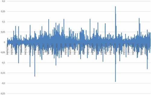
Figures 1 and 2 set out Bitcoin’s hourly closing prices and hourly close-to-close returns in percentages, respectively. We can observe that it is not only upward and downward trends in Bitcoin’s hourly price that lead to notable close-to-close return increases and decreases. These were also seen during the theoretically calm periods of 2016 and 2019 when prices were following a sideways trend. Looking at Figure 2, we can confirm the validity of not using a filter higher that 5% due to the low number of events that exceed that filter size.

Figure 1. Bitcoin hourly prices.

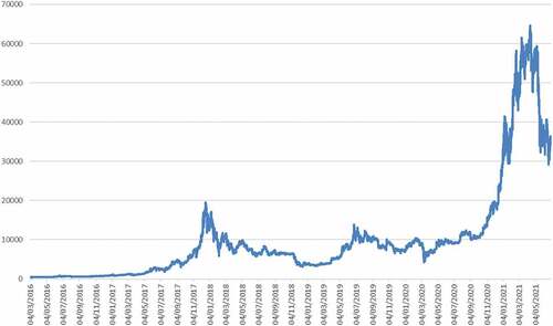
Figure 2. Bitcoin hourly returns.

Our methodology follows the line of such studies analysing price shocks. However, instead of using just a procedure for defining price shocks we employ four different procedures to define them as a way to add greater robustness to our results. We combine classic procedures based on filter sizes with other methodologies focused on technical analysis (the trading range breakout rule, also known as support and resistance levels) and volatility (an approach in the spirit of the Bollinger Bands based on defined percentiles and VaR).

The first procedure follows a standard methodology also used by Fung et al. (2000), Benou and Richie (2003), Grant et al. (2005), Ising et al. (2006), Mazouz, Joseph, and Palliere (2009) and Miralles-Marcelo et al. (2014), where price shocks are defined as returns larger or smaller than a given filter size. Our main reason for using this approach is based on the statement of Fung et al. (2000) who point out that the more extreme the price movement is the greater the subsequent adjustment. Following this approach, an event appears when the hourly return, which is calculated as the log difference of two consecutive closing prices, is larger or smaller than six filter sizes: ±0.5%, ±1%, ±1.5%, ±2.5%, ±3.5% and ±5%. In keeping with Fung et al. (2000), we do not employ filter sizes larger than 5% because the number of events decreases, as does the reliability of the research.

The second approach used for defining price shocks is based on technical analysis and, more precisely, on the trading range breakout rule which is also known as the support and resistance indicator. The main reason that leads us to use it is the fact that since the seminal work by Brock et al. (1992) it has been one of the most popular methods of analysis and has received considerable attention in the literature. Additionally, Brock et al. (1992) show that this rule has significant predictive power for US equity index returns. Their results were confirmed by Yu et al. (2013) for the Malaysian market and Gerritsen et al. (2020) for Bitcoin prices.

Following this procedure, we find a positive shock when the return in hour t is higher than the resistance and a negative shock when the return is lower than the resistance.

(1) $\mathit{Negative}\mathit{shock}\mathit{if}{P}_{\mathit{i},\mathit{t}}⟨\mathit{Min}\left(P_{\mathit{i},\mathit{t}-1},P_{\mathit{i},\mathit{t}-2},\dots ,P_{\mathit{i},\mathit{t}-\mathit{n}}\right)\mathit{Positive}\mathit{shock}\mathit{if}{P}_{\mathit{i},\mathit{t}}⟩\mathit{Max}\left(P_{\mathit{i},\mathit{t}-1},P_{\mathit{i},\mathit{t}-2},\dots ,P_{\mathit{i},\mathit{t}-\mathit{n}}\right)$(1)

Once adapted to our hourly data, this indicator signals minimum and maximum returns for bitcoin over the past n hours (6, 12, 24, 48, 96, 144, and 192 in our case, which represent ranges from a quarter of a day to 8 days). The rationale of using a window is given by Atkins and Dyl (1990) who state that in that way is eliminated any bias caused by calendar effects patterns.

Lasfer et al. (2003) consider that previous approaches are inappropriate because do not take into account the volatility of returns. For that reason, they propose to analyze price overreactions and underreactions after price shocks by using a derivation of the well-known Bollinger Bands technical analysis. This technical trading rule, defined by Bollinger (1992), which measures price volatility, consists of a moving average around which two bands, usually twice the standard deviation of the asset price, are plotted. However, we follow the method used by Lasfer et al. (2003) which is also employed by Caporale and Plastun (2019, 2020) and Plastun et al. (2021) who modify the Bollinger Band approach slightly by considering returns instead of prices.

Therefore, we consider that there is a shock when the return at hour t is above or below the mean return plus or minus k times the standard deviation of the returns. Following the previous methodology, we have denoted positive and negative shocks as:

(2) $\mathit{Positive}\mathit{shock}\mathit{if}{R}_{\mathit{i},\mathit{t}}>\mathit{MA}{\left(R_i\right)}_{\mathit{t},\mathit{n}}+\mathit{k}{\sigma }_{{\mathit{R}}_{\mathit{i},\mathit{n}}}\mathit{Negative}\mathit{shock}\mathit{if}{R}_{\mathit{i},\mathit{t}}<\mathit{MA}{\left(R_i\right)}_{\mathit{t},\mathit{n}}-\mathit{k}{\sigma }_{{\mathit{R}}_{\mathit{i},\mathit{n}}}$(2)

Where $\mathit{MA}{\left(R_i\right)}_{\mathit{t},\mathit{n}}$ is the simple n-hour moving average of returns for Bitcoin at hour t and k is the number of standard deviations ${\sigma }_{{\mathit{R}}_{\mathit{i},\mathit{n}}}$ of the Bitcoin used to define the bands. We employ natural logarithm returns over the previous 6, 12, 24, 48, 96, 144, and 192 hours to estimate moving averages and three bands of 1, 2, and 3 times the standard deviation, allowing more volatility measurements than the classical k = 2 value.

Finally, we opt for also using VaR for defining an event because this is the current standard risk measurement tool which is recommended for turbulent circumstances since Basel II. VaR is a statistic that quantifies the extent of possible financial losses within a firm, portfolio or position over a specific timeframe or, in other words, it is the maximum return expected to be lost over a given time horizon. Its calculation is based on percentiles, so the 95% VaR represents the return forming the boundary for the 5% worst returns, which is the 5th percentile. Thus, we have defined negative shocks as those returns below the 5th, 2nd and 0.5th percentiles estimated over samples for the previous 6, 12, 24, 48, 96, 144, and 192 hours. In contrast, we consider positive shocks as those returns at hour t that are above the returns which mark the 95th, 98th and 99.5th percentiles.

In all cases, once the event has been defined, we follow the procedure proposed by Fung et al. (2000), Grant et al. (2005), Miralles-Marcelo et al. (2014) and more recently Lalwani, Sharma, and Chakraborty (2019), among others, who focus on the significance of average cumulative returns after the events. Therefore, we calculate the cumulative returns (CR_it) as the change in log prices over a time interval. We have considered eight different intervals: 1, 2, 3, 4, 5, 6, 12 and 24 hours following the event.

(3) $\mathrm{C}{\mathrm{R}}_{\mathrm{it}}=\mathrm{Ln}\left({\mathrm{P}}_{\mathrm{it}}\right)-\mathrm{Ln}\left({\mathrm{P}}_{\mathrm{i}0}\right)$(3)

Where P_it and P_i0 are Bitcoin prices on each hour after the event and the closing price of the event, respectively. Following Caporale and Plastun (2020), these returns do not incorporate transaction costs because for internet trading these costs are small and ignoring them does not affect the results.

These cumulative returns are averaged to obtain the average cumulative return as follows:

(4) $\mathrm{ACR}=\frac{1}{\mathrm{N}}\sum _{\mathrm{i}=1}^{\mathrm{N}}\mathrm{C}{\mathrm{R}}_{\mathrm{it}}$(4)

Where N is the number of events corresponding to each filter. A traditional t-test is calculated to test whether these average cumulative returns are significantly different from zero. A positive (negative) and statistically significant value for an ACR after a positive (negative) shock would be consistent with the underreaction hypothesis. However, a negative (positive) and statistically significant value for an ACR after a positive (negative) shock would be consistent with the overreaction hypothesis The t-statistic is obtained as:

(5) $\mathit{t}=\frac{\mathit{ACR}}{\frac{\mathit{\sigma }}{\sqrt{\mathit{N}}}}$(5)

Where σ is the standard deviation of the cumulative returns and N is the number of shocks.

4. Empirical results

Tables 1 and 2 report the 1, 2, 3, 4, 5, 6, 12 and 24-hour average cumulative returns (ACR) following each positive and negative shock, respectively. Following Caporale and Plastun (2020), these returns do not incorporate transaction costs because for internet trading, these costs are small and excluding them does not affect the results.

Table 1. Filter size. Average cumulative returns (Positive shocks).

Shocks (%)	1 H	2 H	3 H	4 H	5 H	6 H	12 H	24 H
0.5	−0.028**	−0.046**	−0.047**	−0.050**	−0.050**	−0.021	0.082**	0.286***
	(−2.201)	(−2.538)	(−2.199)	(−2.036)	(−1.867)	(−0.732)	(2.077)	(5.095)
1	−0.026	−0.051	−0.047	−0.070	−0.080*	−0.051	0.028	0.218**
	(−1.127)	(−1.572)	(−1.240)	(−1.592)	(−1.700)	(−0.994)	(0.408)	(2.236)
1.5	−0.029	−0.034	−0.013	−0.062	−0.034	0.023	0.148	0.391***
	(−0.784)	(−0.696)	(−0.235)	(−0.920)	(−0.468)	(0.284)	(1.363)	(2.594)
2.5	0.003	3·10^−4	0.066	−0.099	−0.038	0.031	0.153	0.504*
	(0.038)	(0.002)	(0.549)	(−0.726)	(−0.254)	(0.192)	(0.725)	(1.713)
3,5	−0.092	−0.049	0.194	0.131	0.160	0.220	−0.112	0.637
	(−0.590)	(−0.257)	(0.949)	(0.591)	(0.647)	(0.830)	(−0.305)	(1.259)
5	−0.243	−0.046	0.537	0.933**	0.684	0.726	0.596	2.001**
	(−0.716)	(−0.109)	(1.279)	(2.191)	(1.396)	(1.311)	(0.765)	(2.054)

This table contains the average cumulative returns in percentages and t-statistics in brackets from each positive shock up to different hourly holding times over the whole sample. Significant coefficients are denoted by ***, ** and * for 1%, 5% and 10% significance levels, respectively.

Table 2. Filter size. Average cumulative returns (Negative shocks).

Shocks (%)	1 H	2 H	3 H	4 H	5 H	6 H	12 H	24 H
0.5	0.071***	0.110***	0.142***	0.135***	0.155***	0.165***	0.180***	0.250***
	(4.540)	(5.283)	(5.800)	(4.894)	(4.968)	(4.955)	(3.997)	(3.908)
1	0.109***	0.199***	0.258***	0.250***	0.254***	0.264***	0.264***	0.357***
	(3.749)	(5.237)	(5.892)	(5.064)	(4.547)	(4.494)	(3.402)	(3.266)
1.5	0.160***	0.277***	0.351***	0.368***	0.381***	0.431***	0.506***	0.655***
	(3.488)	(4.683)	(5.231)	(4.898)	(4.453)	(4.828)	(4.296)	(4.037)
2.5	0.259***	0.542***	0.528***	0.539***	0.607***	0.745***	0.915***	1.320***
	(2.917)	(4.581)	(3.979)	(3.591)	(3.588)	(4.301)	(3.951)	(4.248)
3.5	0.533***	0.996***	0.974***	1.032***	1.200***	1.471***	1.565***	2.299***
	(3.302)	(4.768)	(4.258)	(3.932)	(3.861)	(4.894)	(3.922)	(4.629)
5	0.875**	1.833***	1.664***	1.793***	1.896***	2.394***	2.181**	3.132***
	(2.473)	(3.733)	(3.323)	(3.163)	(2.625)	(3.419)	(2.432)	(2.908)

This table contains the average cumulative returns in percentages and t-statistics in brackets from each negative shock up to different hourly holding times over the whole sample. Significant coefficients are denoted by ***, ** and * for 1%, 5% and 10% significance levels, respectively.

From Table 1 we can observe the mixed behaviour of average cumulative returns after positive shocks. We find evidence that positive shocks of 0.5% are followed by a significant overreaction effect (a negative average cumulative return and a significant t-statistic) up to five hours after the shock. However, the average cumulative return changes to a significant continuation pattern twelve and twenty-four hours after the shock. Furthermore, when larger filters are considered, only a few average cumulative returns are significant.

We find that average cumulative returns show evidence of underreaction effects twenty-four hours after 1%, 1.5%, 2.5% and 5% shocks, but also up to 4 hours after a 5% shock. In contrast, average cumulative returns exhibit a significant overreaction effect in the 5 hours after a 1% shock.

Conversely, in Table 2 we find positive and significant average cumulative returns following negative price shocks for all filters and hours, which is clear evidence of an overreaction effect. We find clear large average cumulative returns when higher filters are employed, but also when the investment is held for a larger number of hours.

Consequently, higher overreaction effects are found six and twenty-four hours after 5% negative shocks, where average cumulative returns of 2.394% and 3.132% respectively are obtained. Average cumulative returns twenty-four hours after a 3.5% negative shock are also similar to the highest ones (2.299%).

Tables 3 and 4 show the average cumulative returns from price shocks following the second approach in which breaks of support and resistance are considered. In accordance with the previous results, we observe that breaking previous resistances (positive shocks) does not lead to significant reactions in the market. We find a continuation pattern up to 24 hours after the shock for all the past return samples considered. Moreover, these underreactions are higher the longer the reference period used to estimate resistance. It is also interesting to note that there are more significant average cumulative returns when resistances from longer reference periods are broken, especially those relating to the previous 144 and 192 hours. In both cases, we find positive and significant average cumulative returns 3 and 5 hours after the shock, and also up to 6 and 12 hours, but only when 192 hours is the reference for estimating the resistance.

Table 3. Trading range breakout rule. Average cumulative returns (Breaking resistances).

Sample	1 H	2 H	3 H	4 H	5 H	6 H	12 H	24 H
6	−0.006	−0.019	0.001	−0.011	−0.009	0.010	0.077**	0.236***
	(−0.579)	(−1.266)	(0.071)	(−0.553)	(−0.413)	(0.398)	(2.171)	(4.630)
16	−0.005	0.001	0.017	−0.006	−0.011	−1.41 · 10^−4	0.046	0.207***
	(−0.301)	(0.058)	(0.677)	(−0.207)	(−0.336)	(−0.004)	(0.959)	(2.972)
24	−0.006	0.011	0.035	0.001	−0.001	0.024	0.098	0.181*
	(−0.251)	(0.364)	(1.008)	(0.029)	(−0.024)	(0.480)	(1.351)	(1.749)
48	0.000	0.077	0.088	0.030	0.065	0.077	0.167	0.333**
	(0.005)	(1.576)	(1.563)	(0.451)	(0.880)	(0.969)	(1.508)	(2.178)
96	0.015	0.103	0.107	0.075	0.159	0.162	0.278*	0.409*
	(0.287)	(1.462)	(1.350)	(0.784)	(1.485)	(1.419)	(1.743)	(1.918)
144	0.036	0.147	0.188*	0.141	0.234*	0.197	0.329	0.481*
	(0.491)	(1.589)	(1.814)	(1.133)	(1.675)	(1.339)	(1.612)	(1.764)
192	0.015	0.128	0.223*	0.216	0.362**	0.298*	0.473*	0.655*
	(0.166)	(1.123)	(1.733)	(1.455)	(2.177)	(1.696)	(1.938)	(1.958)

This table contains the average cumulative returns in percentages and t-statistics in brackets from each positive shock up to different hourly holding times over the whole sample. The first column denotes the number of hours that were considered for determining the resistance level. Significant coefficients are denoted by ***, ** and * for 1%, 5% and 10% significance levels, respectively.

Table 4. Trading range breakout rule. Average cumulative returns (Breaking supports).

Sample	1 H	2 H	3 H	4 H	5 H	6 H	12 H	24 H
6	0.055***	0.087***	0.107***	0.111***	0.126***	0.130***	0.247***	0.271***
	(4.896)	(5.646)	(5.837)	(5.269)	(5.216)	(5.029)	(6.944)	(5.114)
16	0.065***	0.110***	0.127***	0.132***	0.158***	0.171***	0.255***	0.199***
	(3.869)	(4.864)	(4.919)	(4.444)	(4.713)	(4.733)	(5.121)	(2.673)
24	0.082***	0.152***	0.149***	0.152***	0.208***	0.202***	0.194***	0.193*
	(3.226)	(4.642)	(3.932)	(3.514)	(4.236)	(3.867)	(2.659)	(1.774)
48	0.088**	0.144***	0.153**	0.115*	0.179**	0.177**	0.212**	0.211
	(2.238)	(2.810)	(2.622)	(1.682)	(2.337)	(2.161)	(2.020)	(1.465)
96	0.182***	0.313***	0.232**	0.130	0.200*	0.208*	0.124	0.185
	(2.948)	(3.943)	(2.536)	(1.207)	(1.739)	(1.719)	(0.830)	(0.890)
144	0.201**	0.346***	0.223*	0.126	0.228	0.186	0.116	0.032
	(2.364)	(3.238)	(1.808)	(0.868)	(1.490)	(1.150)	(0.577)	(0.120)
192	0.255**	0.483***	0.328**	0.244	0.362*	0.376*	0.359	0.156
	(2.439)	(3.742)	(2.213)	(1.396)	(1.971)	(1.938)	(1.570)	(0.482)

This table contains the average cumulative returns in percentages and t-statistics in brackets from each negative shock up to different hourly holding times over the whole sample. The first column denotes the number of hours that were considered for determining the support level. Significant coefficients are denoted by ***, ** and * for 1%, 5% and 10% significance levels, respectively.

In contrast, Table 4 shows positive and mostly significant average cumulative returns when supports are broken. This is clear evidence of an overreaction effect, but also indicates more reliability when following the signals from negative shocks rather than positive shocks. More precisely, we find that all the estimated average cumulative returns after the breaking of supports based on the previous 6, 16, and 24 hours are statistically significant and almost all from supports estimated considering the previous 48 hours (only average cumulative returns up to 24 hours after the shock are not significant). Furthermore, higher average cumulative returns are obtained when the previous 192 hourly returns are considered. We find that up to 2 hours after breaking the support it is possible to obtain a 0.483% average cumulative return, which falls to 0.376% and 0.362% 6 and 5 hours after the shock, respectively. Despite some average cumulative returns not being statistically significant when longer samples are considered for determining the supports (96, 144, and 192 hours), we consider that the results shown in Tables 3 and 4 reinforce the previous evidence from Tables 1 and 2, where the importance of negative shocks versus positive ones was discussed.

Average cumulative returns estimated from the proposed approach adapting the Bollinger Bands procedure are reported in Tables 5 and 6. Once again, we do not see a large number of significant averages after a positive shock (see Table 5). We find that shocks detected using one standard deviation result in negative and significant average cumulative returns, providing clear evidence of the overreaction effect, 1 hour after the shock when the previous 6, 12, 48, 96, and 144 hourly returns were used to estimate the means and standard deviations. We also find evidence of the overreaction effect up to 2 hours after the shock (48 hours for the mean and 1 standard deviation), 4 hours after the shock (192 hours and 1 standard deviation) and 5 hours after the shock (144 and 192 hours, both with 1 standard deviation). However, these overreactions change to a continuation pattern when the asset is held for longer (12 and 24 hours). In these cases, we observe that most of the average cumulative returns up to 12 hours after the shock are significant for all bands (1, 2, or 3 standard deviations) and all of them are significant 24 hours after the positive shock. In general terms, these average cumulative returns 12 and 24 hours after the shock show higher values than the rest.

Table 5. Average cumulative returns (Returns higher than mean return plus k deviations).

Hours-k	1 H	2 H	3 H	4 H	5 H	6 H	12 H	24 H
6–1	−0.016*	−0.017	0.000	−0.002	0.001	0.019	0.087***	0.270***
	(−1.809)	(−1.364)	(0.026)	(−0.136)	(0.028)	(0.912)	(2.932)	(6.248)
6–2	0.002	0.007	0.023	−0.011	−0.014	0.010	0.084*	0.230***
	(0.155)	(0.336)	(0.982)	(−0.397)	(−0.463)	(0.303)	(1.744)	(3.303)
6–3	0.010	0.041	0.051	0.046	0.058	0.066	0.111	0.258**
	(0.406)	(1.301)	(1.407)	(1.083)	(1.261)	(1.281)	(1.550)	(2.462)
12–1	−0.018*	−0.013	−0.011	−0.021	−0.025	−0.006	0.044	0.259***
	(−1.770)	(−0.915)	(−0.659)	(−1.075)	(−1.125)	(−0.260)	(1.291)	(5.265)
12–2	0.024	0.029	0.044	0.047	0.033	0.054	0.109*	0.318***
	(1.155)	(1.071)	(1.346)	(1.296)	(0.797)	(1.222)	(1.719)	(3.492)
12–3	0.046	0.091**	0.103**	0.158***	0.148**	0.154**	0.232**	0.344**
	(1.306)	(2.009)	(1.944)	(2.697)	(2.286)	(2.208)	(2.254)	(2.322)
24–1	−0.018	−0.020	−0.012	−0.022	−0.028	−0.005	0.068*	0.265***
	(−1.584)	(−1.249)	(−0.652)	(−1.002)	(−1.132)	(−0.196)	(1.785)	(4.842)
24–2	0.023	0.058*	0.066*	0.090**	0.079	0.113**	0.192**	0.408***
	(0.908)	(1.694)	(1.661)	(2.034)	(1.559)	(2.126)	(2.497)	(3.693)
24–3	0.068	0.146**	0.200***	0.256***	0.296***	0.300***	0.351**	0.559***
	(1.350)	(2.405)	(2.886)	(3.390)	(3.540)	(3.276)	(2.516)	(2.946)
48–1	−0.031**	−0.030*	−0.015	−0.024	−0.023	0.006	0.114***	0.337***
	(−2.334)	(−1.656)	(−0.683)	(−0.972)	(−0.860)	(0.204)	(2.774)	(5.757)
48–2	0.046	0.068*	0.080*	0.084	0.106*	0.144**	0.222**	0.473***
	(1.479)	(1.699)	(1.733)	(1.628)	(1.813)	(2.328)	(2.487)	(3.798)
48–3	0.038	0.100	0.145*	0.224***	0.276***	0.308***	0.459***	0.706***
	(0.643)	(1.358)	(1.862)	(2.590)	(2.850)	(2.964)	(3.011)	(3.518)
96–1	−0.028**	−0.029	−0.009	−0.031	−0.037	0.003	0.110**	0.330***
	(−1.994)	(−1.475)	(−0.415)	(−1.195)	(−1.308)	(0.097)	(2.537)	(5.445)
96–2	−0.002	−9.87 · 10^−5	0.023	0.004	0.001	0.065	0.121	0.369***
	(−0.069)	(−0.002)	(0.458)	(0.066)	(0.014)	(0.932)	(1.243)	(2.807)
96–3	−0.006	0.078	0.128	0.222**	0.265**	0.293**	0.410**	0.750***
	(−0.092)	(0.951)	(1.425)	(2.263)	(2.444)	(2.519)	(2.443)	(3.484)
144–1	−0.028*	−0.030	−0.019	−0.042	−0.060**	−0.014	0.090**	0.278***
	(−1.849)	(−1.502)	(−0.804)	(−1.541)	(−2.004)	(−0.437)	(1.998)	(4.424)
144–2	−0.014	−0.003	0.030	−0.009	−0.011	0.016	0.117	0.401***
	(−0.401)	(−0.057)	(0.568)	(−0.159)	(−0.167)	(0.225)	(1.166)	(2.923)
144–3	−0.039	0.056	0.109	0.109	0.178	0.190	0.324*	0.666***
	(−0.566)	(0.641)	(1.125)	(1.026)	(1.515)	(1.503)	(1.776)	(2.816)
192–1	−0.021	−0.029	−0.021	−0.049*	−0.059*	−0.017	0.096**	0.271***
	(−1.370)	(−1.356)	(−0.828)	(−1.673)	(−1.885)	(−0.503)	(2.047)	(4.134)
192–2	−0.025	−0.032	0.017	−0.033	−0.043	−0.011	0.114	0.421***
	(−0.689)	(−0.679)	(0.318)	(−0.540)	(−0.606)	(−0.142)	(1.110)	(2.937)
192–3	−0.049	0.006	0.061	0.030	0.142	0.189	0.276	0.510**
	(−0.680)	(0.064)	(0.604)	(0.265)	(1.150)	(1.466)	(1.409)	(1.980)

This table contains the average cumulative returns in percentages and t-statistics in brackets from each positive shock up to different hourly holding times over the whole sample. The first column denotes the number of hours that were considered for determining the support level and the number of standard deviations (k). Significant coefficients are denoted by ***, ** and * for 1%, 5% and 10% significance levels, respectively.

Table 6. Average cumulative returns (Returns lower than mean return plus k deviations).

Hours-k	1 H	2 H	3 H	4 H	5 H	6 H	12 H	24 H
6–1	0.049***	0.074***	0.099***	0.104***	0.117***	0.122***	0.220***	0.290***
	(4.892)	(5.484)	(6.305)	(5.808)	(5.699)	(5.545)	(7.361)	(6.583)
6–2	0.071***	0.097***	0.125***	0.127***	0.154***	0.164***	0.207***	0.232***
	(4.205)	(4.338)	(4.773)	(4.202)	(4.397)	(4.426)	(4.152)	(3.191)
6–3	0.075***	0.104***	0.125***	0.112**	0.143***	0.159***	0.156**	0.068
	(2.618)	(2.861)	(2.949)	(2.246)	(2.597)	(2.868)	(2.098)	(0.613)
12–1	0.060***	0.090***	0.120***	0.129***	0.145***	0.154***	0.242***	0.245***
	(5.244)	(5.851)	(6.799)	(6.406)	(6.385)	(6.303)	(7.170)	(4.928)
12–2	0.072***	0.121***	0.138***	0.128***	0.150***	0.156***	0.142**	0.118
	(3.229)	(4.039)	(4.082)	(3.272)	(3.480)	(3.359)	(2.238)	(1.238)
12–3	0.061	0.129**	0.155**	0.102	0.154**	0.149*	0.071	−0.195
	(1.496)	(2.279)	(2.547)	(1.405)	(2.033)	(1.858)	(0.648)	(−1.159)
24–1	0.072***	0.108***	0.121***	0.122***	0.132***	0.130***	0.143***	0.183***
	(5.474)	(6.146)	(5.945)	(5.235)	(5.054)	(4.705)	(3.734)	(3.252)
24–2	0.060**	0.119***	0.136***	0.113**	0.146***	0.139**	0.057	0.031
	(2.067)	(3.200)	(3.262)	(2.303)	(2.738)	(2.423)	(0.738)	(0.268)
24–3	0.097*	0.169**	0.174**	0.117	0.117	0.089	−0.061	−0.184
	(1.828)	(2.380)	(2.313)	(1.326)	(1.239)	(0.887)	(−0.450)	(−0.901)
48–1	0.084***	0.117***	0.138***	0.145***	0.160***	0.162***	0.191***	0.211***
	(5.606)	(5.861)	(5.939)	(5.524)	(5.423)	(5.203)	(4.461)	(3.407)
48–2	0.092**	0.153***	0.168***	0.143**	0.217***	0.185***	0.104	0.039
	(2.554)	(3.284)	(3.377)	(2.528)	(3.467)	(2.751)	(1.139)	(0.312)
48–3	0.059	0.133*	0.102	0.073	0.117	0.060	0.048	−0.079
	(0.987)	(1.703)	(1.202)	(0.751)	(1.123)	(0.533)	(0.324)	(−0.361)
96–1	0.079***	0.121***	0.149***	0.152***	0.170***	0.176***	0.196***	0.265***
	(4.816)	(5.434)	(5.860)	(5.327)	(5.267)	(5.171)	(4.311)	(4.096)
96–2	0.105***	0.209***	0.228***	0.191***	0.233***	0.260***	0.233**	0.145
	(2.625)	(4.118)	(3.977)	(2.864)	(3.067)	(3.368)	(2.295)	(1.018)
96–3	0.170**	0.300***	0.242**	0.243**	0.331***	0.330**	0.301*	0.153
	(2.153)	(3.075)	(2.358)	(2.110)	(2.650)	(2.446)	(1.765)	(0.621)
144–1	0.083***	0.135***	0.165***	0.170***	0.187***	0.201***	0.212***	0.283***
	(4.712)	(5.759)	(6.102)	(5.556)	(5.365)	(5.510)	(4.377)	(4.115)
144–2	0.124***	0.264***	0.274***	0.264***	0.314***	0.349***	0.392***	0.333**
	(2.975)	(4.853)	(4.541)	(3.731)	(3.898)	(4.234)	(3.656)	(2.208)
144–3	0.213**	0.397***	0.368***	0.360***	0.516***	0.513***	0.417**	0.312
	(2.482)	(3.665)	(3.170)	(2.745)	(3.565)	(3.344)	(2.195)	(1.153)
192–1	0.087***	0.143***	0.180***	0.180***	0.197***	0.216***	0.209***	0.263***
	(4.748)	(5.896)	(6.419)	(5.710)	(5.458)	(5.731)	(4.198)	(3.708)
192–2	0.167***	0.312***	0.312***	0.319***	0.374***	0.399***	0.447***	0.441***
	(3.779)	(5.426)	(4.924)	(4.352)	(4.471)	(4.688)	(3.945)	(2.817)
192–3	0.207**	0.426***	0.361***	0.367***	0.476***	0.504***	0.422**	0.403
	(2.404)	(3.913)	(2.932)	(2.680)	(3.060)	(3.234)	(2.142)	(1.464)

This table contains the average cumulative returns in percentages and t-statistics in brackets from each negative shock up to different hourly holding times over the whole sample. The first column denotes the number of hours that were considered for determining the support level and the number of standard deviations (k). Significant coefficients are denoted by ***, ** and * for 1%, 5% and 10% significance levels, respectively.

The averages following breaks of the lower band, reported in Table 6, are consistent with overreaction patterns in all cases where they are found to be significant. Once again, the higher number of significant averages after negative shocks compared to those found after positive shocks (Table 5) is a sign of their accuracy. When one standard deviation is used to estimate the lower band, all average returns following negative shocks appear to be significant and most of these are also significant when two standard deviations are used. However, most of the average cumulative returns up to 24 hours are not significant.

Table 6 also reveals that negative shocks have larger average cumulative returns most of the time compared to positive ones. These larger values are concentrated in longer samples for the means and 3 standard deviations for the lower band. We find an average cumulative return of 0.516% up to 5 hours after the shock when the previous 144 hourly returns are considered in calculating the indicator’s mean, a 0.513% average cumulative return up to six hours later using the same 144 hours and a 0.504% average when 192 hours is the reference.

In Tables 7 and 8 we set out the results from analysing the extreme shocks based on different percentiles. As found previously, there are only a few significant average cumulative returns after positive shocks and all of these are found 12 and 24 hours after the shocks. Their positive values show evidence of a continuation pattern after positive shocks.

Table 7. Higher percentiles average cumulative returns (positive shocks).

Hours-Percentiles	1 H	2 H	3 H	4 H	5 H	6 H	12 H	24 H
6–95	−0.009	−0.021	−0.006	−0.014	−0.017	−0.001	0.066**	0.233***
	(−0.902)	(−1.505)	(−0.351)	(−0.751)	(−0.818)	(−0.045)	(2.016)	(4.910)
6–98	−0.004	−0.017	−0.002	−0.014	−0.015	0.005	0.067**	0.230***
	(−0.415)	(−1.144)	(−0.139)	(−0.712)	(−0.675)	(0.222)	(1.938)	(4.628)
6–99.5	−0.006	−0.018	0.001	−0.015	−0.013	0.006	0.071**	0.230***
	(−0.603)	(−1.204)	(0.031)	(−0.743)	(−0.593)	(0.244)	(2.031)	(4.537)
12–95	−0.003	−0.009	−0.001	−0.035	−0.030	−0.010	0.038	0.237***
	(−0.254)	(−0.523)	(−0.064)	(−1.399)	(−1.102)	(−0.333)	(0.897)	(3.934)
12–98	0.002	0.003	0.013	−0.011	−0.018	−0.002	0.039	0.227***
	(0.116)	(0.182)	(0.562)	(−0.427)	(−0.596)	(−0.063)	(0.852)	(3.433)
12–99.5	−0.003	0.004	0.018	−0.007	−0.013	0.001	0.036	0.197***
	(−0.184)	(0.175)	(0.767)	(−0.258)	(−0.413)	(0.038)	(0.743)	(2.861)
24–95	−0.010	−0.004	0.018	0.003	0.002	0.029	0.116**	0.274***
	(−0.686)	(−0.197)	(0.754)	(0.104)	(0.071)	(0.872)	(2.428)	(4.075)
24–98	0.005	0.015	0.029	0.006	−0.001	0.028	0.108*	0.248***
	(0.225)	(0.566)	(0.947)	(0.157)	(−0.014)	(0.633)	(1.700)	(2.753)
24–99.5	−0.008	0.012	0.037	−0.004	−0.005	0.019	0.085	0.191*
	(−0.360)	(0.414)	(1.074)	(−0.099)	(−0.115)	(0.401)	(1.206)	(1.899)
48–95	0.002	−0.014	0.009	−0.029	−0.033	−0.008	0.075	0.276***
	(0.086)	(−0.580)	(0.315)	(−0.860)	(−0.899)	(−0.209)	(1.354)	(3.557)
48–98	0.011	0.019	0.033	0.016	0.015	0.061	0.140*	0.325***
	(0.442)	(0.538)	(0.842)	(0.366)	(0.289)	(1.110)	(1.840)	(3.0789
48–99.5	0.008	0.071	0.074	0.029	0.046	0.073	0.112	0.321**
	(0.225)	(1.570)	(1.449)	(0.479)	(0.652)	(0.985)	(1.090)	(2.261)
96–95	−0.019	−0.019	0.000	−0.027	−0.032	0.002	0.095	0.313***
	(−0.957)	(−0.699)	(0.006)	(−0.724)	(−0.780)	(0.035)	(1.557)	(3.765)
96–98	−0.033	−0.027	−0.002	−0.044	−0.042	0.012	0.130	0.318***
	(−1.090)	(−0.657)	(−0.053)	(−0.825)	(−0.694)	(0.187)	(1.402)	(2.582)
96–99.5	0.021	0.081	0.073	0.066	0.103	0.161	0.140	0.370*
	(0.431)	(1.278)	(1.039)	(0.789)	(1.038)	(1.556)	(0.924)	(1.821)
144–95	−0.020	−0.024	−0.001	−0.029	−0.045	−0.010	0.128**	0.330***
	(−0.944)	(−0.799)	(−0.019)	(−0.710)	(−1.051)	(−0.210)	(1.987)	(3.763)
144–98	−0.027	−0.023	0.030	−0.028	−0.037	0.002	0.098	0.262**
	(−0.787)	(−0.514)	(0.595)	(−0.483)	(−0.564)	(0.029)	(1.007)	(1.973)
144–99.5	−0.003	0.098	0.114	0.059	0.100	0.154	0.082	0.309
	(−0.047)	(1.246)	(1.323)	(0.593)	(0.848)	(1.255)	(0.459)	(1.307)
192–95	−0.016	−0.017	0.006	−0.030	−0.045	−0.012	0.131**	0.334***
	(−0.752)	(−0.533)	(0.151)	(−0.719)	(−1.013)	(−0.253)	(1.998)	(3.740)
192–98	−0.012	0.006	0.065	0.006	0.006	0.039	0.089	0.303**
	(−0.348)	(0.124)	(1.237)	(0.092)	(0.091)	(0.542)	(0.870)	(2.206)
192–99.5	−0.040	0.014	0.012	−0.013	0.034	0.085	0.090	0.286
	(−0.599)	(0.174)	(0.133)	(−0.133)	(0.280)	(0.668)	(0.492)	(1.191)

This table contains the average cumulative returns in percentages and t-statistics in brackets from each positive shock up to different hourly holding times over the whole sample. The first column denotes the number of hours that were considered for determining the percentile and the percentile. Significant coefficients are denoted by ***, ** and * for 1%, 5% and 10% significance levels, respectively.

Table 8. Lower percentiles average cumulative returns (negative shocks).

Hours-Percentiles	1 H	2 H	3 H	4 H	5 H	6 H	12 H	24 H
6–5	0.052***	0.084***	0.106***	0.108***	0.125***	0.129***	0.239***	0.266***
	(4.925)	(5.815)	(6.183)	(5.514)	(5.535)	(5.369)	(7.222)	(5.412)
6–2	0.054***	0.085***	0.104***	0.106***	0.124***	0.129***	0.237***	0.252***
	(4.923)	(5.675)	(5.842)	(5.182)	(5.266)	(5.104)	(6.831)	(4.876)
6–0.5	0.056***	0.088***	0.108***	0.111***	0.127***	0.133***	0.247***	0.267***
	(4.981)	(5.696)	(5.919)	(5.345)	(5.309)	(5.164)	(6.997)	(5.064)
12–5	0.063***	0.100***	0.121***	0.128***	0.143***	0.159***	0.232***	0.208***
	(4.220)	(5.054)	(5.489)	(4.999)	(4.890)	(5.064)	(5.394)	(3.299)
12–2	0.066***	0.105***	0.123***	0.127***	0.145***	0.163***	0.240***	0.200***
	(4.098)	(4.896)	(5.086)	(4.533)	(4.554)	(4.776)	(5.079)	(2.861)
12–0.5	0.065***	0.110***	0.129***	0.133***	0.158***	0.172***	0.258***	0.201***
	(3.884)	(4.894)	(5.040)	(4.527)	(4.768)	(4.795)	(5.239)	(2.739)
24–5	0.072***	0.117***	0.128***	0.124***	0.151***	0.149***	0.143***	0.164**
	(4.216)	(5.185)	(4.941)	(4.142)	(4.436)	(4.143)	(2.898)	(2.281)
24–2	0.080***	0.148***	0.161***	0.175***	0.219***	0.200***	0.158**	0.161*
	(3.506)	(5.053)	(4.924)	(4.637)	(5.117)	(4.360)	(2.466)	(1.695)
24–0.5	0.081***	0.150***	0.161***	0.169***	0.225***	0.223***	0.215***	0.204*
	(3.272)	(4.602)	(4.395)	(4.029)	(4.769)	(4.419)	(3.043)	(1.916)
48–5	0.089***	0.130***	0.144***	0.119***	0.158***	0.158***	0.154***	0.206**
	(4.146)	(4.685)	(4.656)	(3.318)	(3.816)	(3.645)	(2.708)	(2.547)
48–2	0.078***	0.141***	0.161***	0.165***	0.221***	0.212***	0.202***	0.164
	(2.805)	(3.797)	(3.777)	(3.425)	(4.021)	(3.684)	(2.633)	(1.494)
48–0.5	0.094**	0.159***	0.188***	0.160**	0.226***	0.209***	0.235**	0.262*
	(2.520)	(3.188)	(3.492)	(2.525)	(3.190)	(2.739)	(2.379)	(1.936)
96–5	0.101***	0.165***	0.183***	0.177***	0.206***	0.220***	0.212***	0.216**
	(4.320)	(5.370)	(5.342)	(4.435)	(4.462)	(4.607)	(3.359)	(2.461)
96–2	0.140***	0.221***	0.227***	0.216***	0.298***	0.347***	0.323***	0.322**
	(3.910)	(4.642)	(4.373)	(3.658)	(4.401)	(4.916)	(3.465)	(2.511)
96–0.5	0.100*	0.210***	0.218***	0.138	0.211**	0.213**	0.186	0.283
	(1.781)	(2.874)	(2.747)	(1.474)	(2.124)	(2.005)	(1.404)	(1.534)
144–5	0.104***	0.178***	0.203***	0.190***	0.241***	0.258***	0.258***	0.320***
	(4.110)	(5.374)	(5.253)	(4.316)	(4.724)	(4.870)	(3.795)	(3.368)
144–2	0.166***	0.292***	0.281***	0.265***	0.355***	0.382***	0.378***	0.430***
	(4.033)	(5.452)	(4.805)	(3.989)	(4.615)	(4.822)	(3.588)	(3.034)
144–0.5	0.140**	0.261***	0.245**	0.231**	0.298**	0.275**	0.241	0.263
	(2.037)	(2.911)	(2.473)	(2.040)	(2.508)	(2.155)	(1.516)	(1.235)
192–5	0.103***	0.177***	0.204***	0.206***	0.244***	0.273***	0.254***	0.314***
	(3.869)	(5.055)	(5.073)	(4.518)	(4.601)	(4.936)	(3.564)	(3.190)
192–2	0.161***	0.281***	0.252***	0.237***	0.320***	0.348***	0.379***	0.407***
	(3.670)	(4.979)	(4.016)	(3.284)	(3.823)	(4.090)	(3.407)	(2.694)
192–0.5	0.175**	0.279***	0.264**	0.251**	0.307**	0.320**	0.296*	0.217
	(2.400)	(2.885)	(2.420)	(1.989)	(2.163)	(2.249)	(1.684)	(0.931)

This table contains the average cumulative returns in percentages and t-statistics in brackets from each positive shock up to different hourly holding times over the whole sample. The first column denotes the number of hours that were considered for determining the percentile and the percentile. Significant coefficients are denoted by ***, ** and * for 1%, 5% and 10% significance levels, respectively.

In contrast with this weak evidence of underreaction after positive shocks, we observe strong evidence of the overreaction effect after negative shocks which is consistent with the previous results derived from using other approaches. Only 8 out of 168 average cumulative returns are not significant. When the 95^th percentile is considered, all negative shocks show significant positive average cumulative returns and for the 98^th percentile only one of these is not statistically significant. Once again, we find evidence that the overreaction effect increases during the day after negative shocks until it reaches maximum average cumulative returns 12 or 24 hours later. This is also the case when longer samples are considered for estimating the percentiles. Therefore, negative shocks derived from using the 2nd percentile over the previous 144 hourly returns yield a 0.430% average cumulative return 24 hours after the shock. This figure is 0.407% 24 hours after the shock when the previous 192 hourly returns are considered for estimating the 2nd percentile.

The main implication of this study is that using four different approaches we have demonstrated that negative shocks lead to a significant overreaction effect. The larger the shock and the number of days and bands used to define it, the greater the effect. We can specifically highlight that the simplest procedure, filter sizes, leads to higher average cumulative returns compared to the rest of the approaches. Additionally, we find that these overreaction effects do not disappear with the passing of hours, but rather the opposite occurs. In general terms, we observe that the average cumulative returns are higher as time passes, even 24 hours after the event when most of them are statistically significant. In contrast, it has been shown that positive shocks do not cause a consistent herding behaviour in investors that leads to an increase in Bitcoin’s value. We generally find an initial overreaction after positive shocks, which results in price falls, but this later changes to an underreaction effect for up to 12 or 24 hours after the shock, but not a very important one in terms of significance levels.

Our results do not coincide with those of Caporale and Plastun (2019), who find evidence of an overreaction effect after positive shocks, defined by returns higher than mean returns plus different standard deviations. However, it should be noted that the time horizons are different because they focus on daily data while we focus on intraday data. A similar conclusion is extracted when our results are compared with those obtained by Caporale and Plastun (2020), where they used the same procedure as the previous one but considering both positive and negative shocks and hourly and daily data. In this case, they show the existence of an overreaction effect after positive shocks but a momentum effect following negative ones. From our point of view, these differences could be caused by the fact that the samples are different in each study, the one used in our study being characterised by some sharper increases and decreases that Caporale and Plastun (2020) do not consider. However, there are more similarities with the results obtained by Kellner and Maltritz (2022). Once again, daily data are used but these are closer to our sample (their sample starts on 1 January 2015 and ends on 31 December 2020 while ours is from 1 March 2016 to 30 June 2021) and show evidence of highly significant overreaction after negative shocks.

Focusing on the economic implications of our findings, we are able to state that a profitable strategy is feasible based simply on investing in Bitcoins after large negative shocks due to the significant positive average cumulative returns. Since we have focused only on the significance of average cumulative returns after the events, following the procedure proposed by Fung et al. (2000), Grant et al. (2005), Miralles-Marcelo et al. (2014) and more recently Lalwani et al. (2019), among others, as pointed out previously, analysing a trading strategy is a future research objective that could be complemented by also considering other cryptocurrencies. We could also focus on analysing whether these overreactions and underreactions are statistically significant using different sub-samples rather than just the whole sample (2016–2021) or whether these results are biased by calendar effects.

5. Conclusions

The objective of this article has been to enrich the evidence on the behaviour of Bitcoin prices after extreme market movements using four different procedures of which only one had been used in a limited manner. This research is justified by the fact that high frequency trading, of which bitcoin is a leading example, dominates the trading scene in today’s modern financial markets. It is also important to help not only professional investors but also at-home traders to capture price fluctuations and develop a framework capable of improving their investing.

We analyse the average cumulative returns on Bitcoin up to specific numbers of hours after different positive and negative shocks. After employing four different approaches, we find mixed results after positive shocks but most of these are not significant. In contrast, we find significant overreaction effects after negative shocks, especially following larger ones and even 24 hours after the shock. From our point of view, these results suggest that investors should focus on negative shocks instead of positive ones because the latter do not lead to a subsequent upward trend, as one might think, but instead can even follow a downward trend in the hours following the shock and they are also mostly not statistically significant. In contrast, the much more uniform behaviour of Bitcoin after negative shocks should reduce the fears of investors and allow them to take some profit from the statistically significant overreaction effect.

These findings have important economic implications because show that investors would be able to develop a profitable trading strategy just focusing on investing after negative shocks avoiding complex methodologies. However, it may prove interesting in future research to use alternative procedures and to look at how they perform when implemented through investment strategies or considering calendar effects.

Author contributions

This work is an outcome of the joint efforts of the two authors. J.L.M.-Q. conceived the research idea, provided research materials, analysis tools and contributed to the interpretation of the results. M.M.M.-Q. conceived the research idea, reviewed the related literature and contributed to the interpretation of the results. Both authors provided contributions to the conclusions and implications of the research and wrote the manuscript and thoroughly read and approved the final version. All authors have read and agreed to the published version of the manuscript.

Data availbility

Data are available at http://dx.doi.org/10.17632/b5sj3r5mzw.1

Disclosure statement

No potential conflict of interest was reported by the author(s).

Additional information

Funding

The authors gratefully acknowledge support from the Junta de Extremadura (Counselling of Economy, Science and Digital Agenda) and the European Regional Development Fund (“A way of doing Europe”) through grant GR21019.

References

- Atanasova, C. V., & Hudson, R. S. (2010). Technical trading rules and calendar anomalies. Are they the same phenomena? Economic Letters, 106(2), 128–130.
- Atkins, A. B., & Dyl, E. (1990). Price reversals, bid-ask spreads, and market efficiency. Journal of Financial and Quantitative Analysis, 25(4), 535–547.
- Benou, G., & Richie, N. (2003). The reversal of large stock price declines: The case of large firms. Journal of Economics and Finance, 27(1), 19–38.
- Blackburn, D. W., & Cakici, N. (2017). Overreaction and the cross-section of returns: International evidence. Journal Empirical Finance, 42, 1–14.
- Bley, J., & Saad, M. (2020). An analysis of technical trading rules: The case of MENA markets. Finance Research Letters, 33, 101182.
- Bodie, Z., Kane, A., & Marcus, A. J. (2018). Investments. New York: McGraw-Hill Education.
- Bogards, O., & Czudaj, R. L. (2020). The prevalence of price overreactions in the cryptocurrency market. Journal of International Financial Markets, Institutions and Money, 65, 101194.
- Bogards, O., & Czudaj, R. L. (2021). Features of overreactions in the cryptocurrency market. The Quarterly Review of Economics and Finance, 80, 31–48.
- Bogards, O., Czudaj, R. L., & Van Hoang, T. H. (2021). Price overreactions in the commodity futures market: An intraday analysis of the Covid-19 pandemic impact. Resources Policy, 71, 101966.
- Bollinger, J. (1992). Using Bollinger Bands. Technical Analysis of Stocks and Commodities, 10(2), 47–51.
- Bouri, E., Lau, C. K. M., Saeed, T., Wang, S., & Zhao, Y. (2021). On the intraday return curves of Bitcoin: Predictability and trading opportunities. International Review of Financial Analysis, 76, 101784.
- Bremer, M. A., & Sweeney, R. J. (1991). The reversal of large stock-price decreases. Journal of Finance, 46(2), 747–754.
- Brock, W., Lakonishok, J., & LeBaron, B. (1992). Simple technical trading rules and the stochastic properties of stock returns. The Journal of Finance, 47(5), 1731–1764.
- Caporale, G. M., Gil-Alana, L., & Plastun, A. (2019). Long-term price overreactions: Are markets inefficient? Journal of Economics and Finance, 43(4), 657–680.
- Caporale, G. M., & Plastun, A. (2019). Price overreactions in the cryptocurrency market. Journal of Economic Studies, 46(5), 1137–1155.
- Caporale, G. M., & Plastun, A. (2020). Momentum effects in the cryptocurrency market after one-day abnormal returns. Financial Markets and Portfolio Management, 34(3), 251–266.
- Caporale, G. M., & Zekokh, T. (2019). Modelling volatility of cryptocurrencies using Markov-switching GARCH models. Research in International Business and Finance, 48, 143–155.
- Chang, J. E., Lima, E. J. A., & Tabak, B. M. (2004). Testing for predictability in emerging equity markets. Emerging Market Review, 5(3), 295–316.
- Chen, J., Zhou, Y., & Wang, X. (2018). Profitability of simple stationary technical trading rules with high-frequency data of Chinese index futures. Physica A: Statistical Mechanics and Its Applications, 492, 1664–1678.
- Corbet, S., Lucey, B., Urquhart, A., & Yarovaya, L. (2019). Cryptocurrencies as a final asset: A systematic analysis. International Review of Financial Analysis, 62, 182–199.
- Cox, D. R., & Peterson, D. R. (1994). Stock returns following large one day declines. evidence on short-term reversals and longer term performance. Journal of Finance, 49(1), 255–267.
- De Bondt, W. F. M., & Thaler, R. H. (1985). Does the stock market overreact? The Journal of Finance, 40(3), 793–805.
- Diaconaşu, D. E., Mehdian, S., Stoica, O. . (2022). An analysis of investors’ behavior in Bitcoin market. Plos One, 17(3), e0264522.
- Fabozzi, F. J., Ma, C. K., Chittenden, W. T., & Pace, R. D. (1995). Predicting intraday price reversals. The Journal of Portfolio Management, 21(2), 42–53.
- Fama, E. F. (1965). The behavior of stock market prices. Journal of Business, 36(1), 34–105.
- Fama, E. F. (1970). Efficient capital markets: A review of theory and empirical work. The Journal of Finance, 25(2), 383–417.
- Fung, A. K., Mok, D. M. Y., & Lam, K. (2000). Intraday price reversals for index futures in the US and Hong Kong. Journal of Banking and Finance, 24(7), 1179–1201.
- Gerritsen, D. F. (2016). Are chartists artists? The determinants and profitability of recommendations based on technical analysis. International Review of Financial Analysis, 47, 179–196.
- Gerritsen, D. F., Bouri, E., Ramezanifar, E., & Roubaud, D. (2020). The profitability of technical trading rules in the Bitcoin market. Finance Research Letters, 34, 101263.
- Gkillas, K., & Katsiampa, P. (2018). An application of extreme value theory to cryptocurrencies. Economic Letters, 164, 109–111.
- Grant, J. L., Wolf, A., & Yu, S. (2005). Intraday price reversals in the U.S. stock index futures market: A 15-Year Study. Journal of Banking and Finance, 29(5), 1311–1327.
- Himmelmann, A., Schiereck, D., Simpson, M. W., & Zschoche, M. (2012). Long-term reactions to large stock price declines and increases in the European stock market: A note on market efficiency. Journal of Economics and Finance, 36(2), 400–423.
- Hudson, R., & Urquhart, A. (2021). Technical trading and cryptocurrencies. Annals of Operations Research, 297(1–2), 191–220.
- Ising, J., Schiereck, D., Simpson, M., & Thomas, T. (2006). Stock returns following large 1-month declines and jumps: Evidence of over optimism in the German market. The Quarterly Review of Economics and Finance, 46(4), 598–619.
- Jegadeesh, N., & Titman, S. (1993). Returns to buying winners and selling losers: Implications for stock market efficiency. Journal of Finance, 48(1), 65–92.
- Kellner, T., & Maltritz, D. (2022). A broad analysis of short-term overreactions in the market for cryptocurrencies. Journal of Economic Studies, 49(8) In Press, 1585–1608.
- Kolaric, S., Kiesel, F., & Schiereck, D. (2016). Return patterns of South Korean stocks following large price shocks. Applied Economics, 48(2), 121–132.
- Lalwani, V., Sharma, U., & Chakraborty, M. (2019). Investor reaction to extreme shocks in stock markets: A cross country examination. IIMB Management Review, 31(5), 258–267.
- Larson, S. J., & Madura, J. (2003). What drives stock price behavior following extreme one-day returns. Journal of Financial Research, 26(1), 113–127.
- Lasfer, M. A., Melnik, A., & Thomas, D. C. (2003). Short-term reaction of stock markets in stressful circumstances. Journal of Banking & Finance, 27(10), 1959–1977.
- Lento, C., & Gradojevic, N. (2022). The profitability of technical analysis during the COVID-19 market meltdown. Journal of Risk and Financial Management, 15(5), 192.
- Lento, C., Gradojevic, N., & Wright, C.S. (2007). Investment information content in Bollinger Bands? Applied Financial Economic Letters, 3(4), 263–267.
- Liu, W., Huang, X., & Zheng, W. (2006). Black-Scholes’ model and Bollinger bands. Physica A: Statistical Mechanics and Its Applications, 371(2), 565–571.
- Li, Y., Urquhart, A., Wang, P., & Zhang, W. (2021). MAX momentum in cryptocurrency markets. International Review of Financial Analysis, 77, 101829.
- Liu, Y., Tsyvinski, A. . (2021). Risks and returns of cryptocurrency. The Review of Financial Studies, 34(6), 2689–2727.
- Maher, D., & Parikh, A. (2011). Short-term under/overreaction, anticipation or uncertainty avoidance? Evidence from India. Journal of International Financial Markets, Institutions and Money, 21(4), 560–584.
- Marshall, B. R., & Cahan, R. H. (2005). Is technical analysis profitable on a stock market which has characteristics that suggest it may be inefficient? Research in International Business and Finance, 19(3), 384–398.
- Marshall, B. R., Qian, S., & Young, M. (2009). Is technical analysis profitable on US stocks with certain size, liquidity or industry characteristics? Applied Financial Economics, 19(15), 1213–1221.
- Mazouz, K., Joseph, N. L., & Palliere, C. (2009). Stock index reaction to large price changes: Evidence from major Asian stock indexes. Pacific-Basin Finance Journal, 17(4), 444–459.
- Mensi, W., Al-Yahyaee, K. H., Al-Jarrah, I. M. W., Vo, X. V., & Kang, S. H. (2020). Dynamic volatility transmission and portfolio management across major cryptocurrencies: Evidence from hourly data. The North American Journal of Economics and Finance, 54, 101285.
- Miralles-Marcelo, J. L., Miralles-Quirós, J. L., & Miralles-Quirós, M. M. (2010). Intraday linkages between the Spanish and the US stock markets: Evidence of an overreaction effect. Applied Economics, 42(2), 223–235.
- Miralles-Marcelo, J. L., Miralles-Quirós, J. L., & Miralles-Quirós, M. M. (2014). Intraday stock market behavior after shocks: The importance of bull and bear markets in Spain. Journal of Behavioral Finance, 15(2), 144–159.
- Naeem, M. A., Bouri, E., Peng, Z., Shahzad, S. J. H., & Vo, X. V. (2021). Asymmetric efficiency of cryptocurrencies during COVID19. Physica A: Statistical Mechanics and Its Applications, 565, 125562.
- Pele, D. T., Wesselhöfft, N., Härdle, W. K., Kolossiatis, M., & Yatracos, Y. G. (2022). Are cryptos becoming alternative assets? The European Journal of Finance. In Press. doi: 10.1080/1351847X.2021.1960403.
- Piccoli, P., Chaudhury, M., & Souza, A. (2017b). How do stocks react to extreme market events? Evidence from Brazil. Research in International Business and Finance, 42, 275–284.
- Piccoli, P., Chaudhury, M., Souza, A., & Vieira da Silva, W. (2017a). Stock overreaction to extreme market events. The North American Journal of Economics and Finance, 41, 97–111.
- Plastun, A., Sibande, X., Gupta, R., & Wohar, M. E. (2021). Evolution of price effects after one-day abnormal returns in the US stock market. The North American Journal of Economics and Finance, 57, 101405.
- Resta, M., Pagnottoni, P., & De Giuli, M. E. (2020). Technical análisis on the bitcoin market: Trading opportunities or investors’ pitfall. Risks, 8(2), 44.
- Samuelson, P. (1965). Proof that properly anticipated prices fluctuate randomly. Industrial Management Review, 6(2), 41–49.
- Shahzad, S. J. H., Bouri, E., Ahmad, T., & Naeem, M. A. (2022). Extreme tail network analysis of cryptocurrencies and trading strategies. Finance Research Letters, 44, 102106.
- Singh, J. E., Babshetti, V., & Shivaprasad, H. N. (2022). Efficient market hypothesis to behavioral finance: A review of rationality to irrationality. Materialsroday: Proceedings. In Press. 10.1016/j.matpr.2021.03.318.
- Spyrou, S., Kassimatis, K., & Galariotis, E. (2007). Short-term overreaction, underreaction and efficient reaction: Evidence from the London Stock Exchange. Applied Financial Economics, 17(3), 221–235.
- Tan, S., Lai, M., Tey, E., & Chong, L. (2020). Testing the performance of technical analysis and sentiment-TAR trading rules in the Malaysian stock market. The North American Journal of Economics and Finance, 51, 100895.
- Tian, G. G., Wan, G. H., & Guo, M. Y. (2002). Market efficiency and the returns to simple technical trading rules: New evidence from U.S. equity market and Chinese equity markets. Asia-Pacific Financial Markets, 9(3/4), 241–258.
- Titan, A. G. (2015). The efficient market hypothesis: review of specialized literature and empirical research. Procedia Economics and Finance, 32, 442–449.
- Troster, V., Tiwari, A. K., Shahbaz, M., & Macedo, D. N. (2019). Bitcoin returns and risk: A general GARCH and GAS analysis. Finance Research Letters, 30, 187–193.
- Tzouvanas, P., Kizys, R., & Tsend-Ayush, B. (2020). Momentum trading in cryptocurrencies: Short-term returns and diversification benefits. Economics Letters, 191, 108728.
- Vidal-Tomás, D. (2021). An investigation of cryptocurrency data: The market that never sleeps. Quantitative Finance, 21(12), 2007–2024.
- Wang, J., Bouri, E., & Ma, F. 2022. “Which factors drive bitcoin volatility: Macroeconomic, technical, or both?” SSRN Working Paper. 10.2139/ssrn.4080107
- Wen, Z., Bouri, E., Xu, Y., & Zhao, Y. (2022). Intraday return predictability in the cryptocurrency markets: Momentum, reversal, or both. The North American Journal of Economics and Finance, 62, 101733.
- Yarovaya, L., Matkovskyy, R., & Jalan, A. (2021). The effects of a black swan event (COVID-19) on herding behavior in cryptocurrency markets. Journal of International Financial Markets, Institutions and Money, 75, 101321.
- Yu, H., Nartea, G. V., Gan, C., & Yao, L. J. (2013). Predictive ability and profitability of simple technical trading rules: Recent evidence from Southeast Asian stock markets. International Review of Economics and Finance, 25, 356–371.
- Zaremba, A., Bilgin, M. H., Long, H., Mercik, A., & Szczygielski, J. J. (2021). Up or down? Short-term reversal, momentum, and liquidity effects in cryptocurrency markets. International Review of Financial Analysis, 78, 101908.
- Zhang, Y., Chan, S., & Nadarajah, S. (2019). Extreme value analysis of high-frequency cryptocurrencies. High Frequency, 2(1), 61–69.