Cartographic content analysis of compelling climate change communication

ABSTRACT

Maps are a key way to communicate climate change. The goal of these maps is to make climate change relatable, tangible, and understandable. However, little research has assessed the content of these maps and the aspects of these maps which attract readers, reduce complexity, and make climate change tangible. One way to evaluate maps of climate change is through the concept of vividness, a term from the communication literature. This article examines the content and vividness of maps of climate change to answer the following: which media organizations publish these maps? What is the design and content of these maps? Did these maps convey climate change vividly? Using content analysis and multidimensional scaling (nMDS) this research showed that producers of climate change maps are often not the publishers of this same content. These maps primarily showed topics which were relevant to audiences in the United States. There was a wide variety of different cartographic designs used. And finally, maps were vivid when they employed the eight aspects of vividness presented in this paper: legend design, symbolization, layout, projections which were appropriate for the data, visual salience, visible change over time, color use which aligned with color connotations, and novel design styles.

KEYWORDS:

• Map design
• climate change communication
• media maps
• cartography
• content analysis
• vividness
• data journalism

1. Introduction

Climate change is a multidimensional and complex issue which has significant and unpredictable impacts on the environment and society (Intergovernmental Panel on Climate Change [IPCC], 2014). Communicating this issue is necessary for better understanding of the causes and impacts of a changing climate. In public communication of climate change, maps have become a common graphic used to communicate information about climate change. The geographic nature of climate change due to the spatial heterogeneity of the causes, impacts, public opinion, and mitigation and adaptation strategies means maps are an effective visual representation for climate change.

Maps of climate change are designed and used by climate scientists, government agencies, as well as journalists in the media, albeit with different audiences in mind. While the specific goals of the maps designed by these groups are different, the overarching goal of these maps remains the same: to make this complex issue relatable, tangible, and understandable for a broad audience. However, little research has assessed the content of these maps and the aspects of these maps which attract readers, reduce complexity, and make the issue of climate change tangible.

One way to evaluate maps of climate change is through the concept of vividness, a term used to describe content that is “likely to attract and hold our attention and to excite the imagination to the extent that it is (a) emotionally interesting, (b) concrete and image provoking, and (c) proximate in a sensory, temporal, or spatial way” (Nisbett & Ross, 1980, p. 45). The term vividness was a popular term used in the fields of advertising, media, and psychology in the late 1970s and 1980s. Vivid content in this prior research often referred to written or spoken content and is theorized to have a “significant impact on message success” (Guadagno et al., 2011, p. 636).

Vividness offers a means of examining the power of maps to influence thinking about an issue. In mapping climate change, journalists have goals of illustrating the changing climate with influential visuals, often maps. Understanding who creates these maps and how these individuals and groups make these maps vivid or not is important for evaluating the power of maps. This article examines the vividness of maps of climate change and answers three core questions:

1. Which media organizations created and shared these maps and were they produced in-house or reproduced from other sources?

2. What aspects of climate change did these maps portray and what aspects of cartographic design did these maps employ?

3. Did these maps convey climate change vividly and which organizations produced the most vivid maps?

2. Background

2.1. Climate change communication

The invisible causes, distant impacts, delayed or absent gratification for action, complexity and uncertainty of the science and the impacts, and our own self-interests toward the status quo all pose challenges to communicating climate change (Moser, 2010; Nerlich et al., 2010). Much of the communication and education literature related to this topic posits a progression from information, to awareness, to concern, and finally to a response or action. As long as people still fail to act, communication is needed to inform about causes, impacts, public opinions, and mitigation and adaptation strategies. For someone to engage in an action to mitigate or adapt to climate change, the person must first have information and be aware of the issue. However, research has illustrated that information alone to raise awareness about climate change is not always sufficient for behavior change, but it is still a necessary component (Chess & Johnson, 2007). The effectiveness of climate change information is limited by the quality of the information and how it is framed (O’Neill & Nicholson-Cole, 2009), the person’s emotions (Joffe, 2008; Otieno et al., 2014; Swim & Bloodhart, 2015) and connection to the environment (Schultz, 2002), as well as their stage of knowledge or behavior change (unawareness, awareness, concern, and response) (Chess & Johnson, 2007; Nerlich et al., 2010).

Much of the research in climate change communication has focused on the media as the primary actor for communicating climate change (Boykoff and Boykoff 2007; Weingart et al., 2000), and indeed, the media is one of the key ways in which information about climate change is communicated to the public (Hannigan, 2014). In addition, visual communication research has illustrated that graphics and pictures are vital components of this communication (Harold et al., 2016; Van der Linden et al., 2014). Visuals can both reduce complexity and help the public understand climate change (Boykoff and Boykoff 2007; DiFrancesco & Young, 2011, Manzo 2012; Smith & Joffe, 2009; Weingart et al., 2000), and some recent research has even established guidelines on effective visual communication of climate change (Harold et al., 2016).

2.2. Cartographic climate change communication

While visuals have been shown to be important for climate change communication, and despite that geographers have focused extensively on climate change in other sub-fields, only a small set of research has focused on map design related to climate change. The majority of this research has focused on identifying best practices for displaying uncertainty (Johannsen et al., 2018; Kaye et al., 2012; Retchless & Brewer, 2016). In addition, other research has critiqued map design used in the IPCC reports (McKendry & Machlis, 2008) focused on map design principles, while other more recent research has connected other topics common in climate change communication, such as motivated reasoning and spatial optimism bias, to how map readers viewed risks to sea level rise (Retchless, 2018).

2.3. Vividness

Information presented in different ways may have an influence on the persuasiveness of a message and how lasting the persuasive content is with the reader. Vivid information is content which is “likely to attract and hold our attention and to excite the imagination to the extent that it is (a) emotionally interesting, (b) concrete and image provoking, and (c) proximate in a sensory, temporal, or spatial way” (Nisbett & Ross, 1980, p. 45). In other words, vivid content brings concepts to life. Vividness has been theorized and shown to be persuasive (e.g. Guadagno et al., 2011). Other reasons include that vivid content is more memorable and thus more cognitively accessible (Eaton, 2011; McGill & Anand, 1989; Shedler & Manis, 1986), meaning readers can incorporate the content into inferences and decisions they make. Vividness may also increase a readers’ ability to construct mental images and recall information through its emotional interest. Indeed, vividness has been shown to increase comprehension (Kelley et al., 1989) and with its ability to attract attention may also lead to greater motivation. Communicators often use vivid content with the goal of influencing their readers. While it is not completely clear why or how this information leads to changes in attitudes and behaviors, a necessary first step is to identify how communicators make information vivid and second to test its potential for persuasion.

2.4. Vivid maps

While the term vivid is rarely, if ever, used in the cartographic realm, attention, emotion, salience and persuasion are common themes within the cartographic literature (e.g. Fabrikant et al., 2012; Fabrikant & Goldsberry, 2005; Griffin & McQuoid, 2012; Muehlenhaus, 2012, 2013, 2014). I argue that maps are vivid through their cartographic design and through the emotions they evoke in their readers. The use of the visual variables (Bertin, 1983), interactive primitives (Roth, 2013), and dynamic variables (DiBiase et al., 1992), well known in cartographic literature, can influence the esthetics of the design and readers’ reactions to the display. Through its potential to influence attitudes, vividness is also aligned with persuasiveness, a focus of some cartographic research in the late 1970s and early 1980s (Tyner, 1982) and again more recently (Muehlenhaus, 2012, 2013, 2014). Additionally, the design of graphics has been shown to influence whether a reader reacts with a greater willingness to engage or disengage in a behavior or attitude (Joffe, 2008; Lang et al., 1993). Vividness may provide a connection between the design of the map, emotion, attention, and persuasion.

3. Methods

This study employed quantitative content analysis to answer the research questions. I assessed the design of 242 maps of climate change. I present the methods of data collection and analysis in this section.

3.1. The sample

Between early 2015 and late 2017, a group of four undergraduate interns under my direction collected maps of climate change. The goal was to find maps in the print and online media published between January 2012 and December 2017 that illustrated climate change causes (e.g. CO₂ production and movement), impacts including everything from temperature and precipitation changes to glacial melt and sea level rise, as well as maps which illustrated the geographic disparities in public opinions about climate change. To be included in the sample of maps, the map needed to clearly indicate that it illustrated climate change in the title, legend, or map notes, or the article needed to mention the term climate change in the text.

The print and online media included in the search did not include maps on personal blogs, maps from peer-reviewed articles, maps in reports for lawmakers (e.g. the IPCC reports), or government agency maps unless these were reproduced in print or online media sources. The sources that were included were newspapers (e.g. The New York Times and The Washington Post) and magazines (e.g. National Geographic Magazine), as well as new digital media (e.g. Buzzfeed, Mashable, etc.).

The maps were located through Internet searches (Google and Twitter), National Geographic Magazine repositories, The New York Times website, The Washington Post website, The Los Angeles Times website, the PressReader database, the Associate Press (AP) Image Database, and The New York Times Historical Database. I used the following search terms across all of these websites and databases: “climate change,” “climate change map,” and “global warming,” as well as more specific terms such as: “sea level rise,” “sea ice,” “glaciers,” “flooding,” “temperature change,” and “precipitation change.” I also used more general search terms including “climate” and “environment.”

PressReader, The New York Times Historical, and the Associated Press (AP) Image databases were available through university library subscriptions. PressReader is a subscription-based service to which libraries can subscribe and allows patrons to browse in full-color the past 90 days of over 6,000 periodical publications from around the globe. Within PressReader I focused on publications in English from the United States from cities with major newspapers. Since this resource only contains the previous 90 days of content, I looked at this source three times: in September 2016, January 2017, and April 2017.

The AP provides news stories to other news organizations. Generally small local newspapers do not produce their own stories and graphics on larger international topics, such as climate change. Instead these smaller outlets rely on the AP for broad non-local stories because the AP has the resources to write these stories with the goal of dissemination through smaller local news organizations. Thus, the graphics from the AP database served as a representation of a wider range of sources.

I also had access to every map published in National Geographic Magazine during the time period of interest, and I identified the maps during that period which illustrated climate change.

Finally, after the initial set was compiled, maps within the same article which had the same design and topic and only illustrated different geographic areas were only coded once in the analysis. For instance, if one website contained maps of sea level rise for five US cities, this was coded as one map because the topic and map design was the same, even if the geographic area of interest in the five maps were different. The final set of maps amounted to 242.

3.2. Content analysis

I analyzed the maps with content analysis. Content analysis is a systematic method for examining and comparing symbols of communication (Rose, 2012). A set of codes is identified and these codes offer a systematic lens by which to examine themes (Krippendorff, 2013). This type of analysis has typically been used for analysis of text, but has recently been expanded to maps to derive common themes (Muehlenhaus, 2011, 2013) as well as best practices (Kessler & Slocum, 2011; Roth et al., 2015).

The goal of this content analysis was to understand who produced the maps, where they were reproduced, what aspect of climate change they illustrated, what types of design they used (type of map and visual variables used), what location and extent they showed, and the extent to which each map was vivid through a Likert scale rating by two coders.

Once the full set of 242 maps was compiled, I established a coding scheme. The coding scheme consisted of general codes (Table 1) and vividness codes (Table 2). The general codes were important for understanding the content included in the maps related to: 1) the publication location, 2) producer, 3) date of publication, 4) use of dynamic map designs, 5) type of map design, and 6) aspect or impact displayed. The vividness codes are: 1) visual salience 2) visible change over time, 3) color use which aligns with cultural and emotional conventions, 4) symbology design, 5) projection, 6) legend design, 7) layout, and 8) novel design use. These codes were established from another study using interviews with 16 mapmakers at government agencies where interviewees indicated that these eight elements were key aspects for making maps of climate change that resonated with audiences (Fish, 2020).

Table 1. List of the general codes and how they were collected.

Code	Data Type
Location	Short Answer
Producer	Short Answer
Date	Date
How dynamic is the map?	Multiple Choice
Type	Multiple Choice
Topic	Short Answer

Table 2. List of the vividness codes and explanations.

Codes	Ratings (5- point Likert Scale)
Visual Salience	Is the important thematic data made salient in the map?
Change over Time	Does the map show change over time to make climate change tangible?
Novel Design	Does the map use a novel design style?
Color Use	Does the map use saturated colors that align with color connotations?
Projection	Does the map use an appropriate projection for the data?
Symbolization	Does the map use visual variables that are appropriate for the data?
Legend Design	Is the legend clear?
Layout	Is the layout design balanced?

We first coded the maps based on the general codes using a Google form. We typed in responses for the short answer codes (Location, Producer, and Topic), a six-digit date for the Date code, and selected from a set of potential answers for the multiple-choice codes. The multiple-choice options for “how dynamic is the map?” were: 1) static, 2) animated, 3) interactive, and 4) both interactive and animated. The “Type” code had the following multiple-choice options: bar graph, cartogram, choropleth, filled isoline, hexbins, line symbol, point symbol, proportional line, proportional symbol, raster, reference, small multiples, and other.

The vividness scores were coded on a 5-point Likert scale where the highest score was assigned if the map fully implemented a particular vividness aspect, and the lowest score was assigned if the map did not engage with a particular aspect (Table 2). The resulting table from the vividness scores looked similar to Table 3.

Table 3. Example output data table of vividness coding.

Map Code	Salience	Change	Novelty	Color	Projection	Symbol	Legend	Layout
001	1	1	1	2	1	1	2	1
002	3	4	2	5	3	1	2	5
003	4	1	5	2	3	2	2	3
004	2	4	5	3	2	2	1	1
005	5	5	5	5	5	5	5	5

3.3. Interrater reliability

The maps were coded by two coders trained in the coding scheme. Both coders coded every map for the general codes and the vividness codes. I measured Cohen’s Kappa and percent agreement to assure interrater reliability. Percent agreement accounts for the differences in coding, while Cohen’s Kappa accounts for agreement that could be expected by chance (Landis & Koch, 1977).

3.4. Non-metric multidimensional scaling (nMDS)

Because the result of the vividness ratings was a combination of the eight vividness aspects, it was important to analyze these codes with a method designed for analyzing multidimensional data. I used non-metric multidimensional scaling (nMDS) in the vegan package in the R statistical software to identify clusters of maps based on vividness codes. nMDS is a visual ordination method used for understanding and explaining the interaction between variables. It is often used by ecologists for understanding species distributions (McCune et al., 2002). As a visual ordination method, nMDS graphics are meant to be read and interpreted visually. The multidimensionality of the input data is scaled to reduce the dimensions, and the resulting dimensions in the nMDS plot are arbitrary. In this case, the eight vividness attributes were scaled to 2D space. This type of analysis does not show the most and least vivid maps, instead it allows readers to see how maps cluster. I created multiple plots to better understand how different maps by different producers and with different designs clustered based on some of the general codes.

4. Results and discussion

This section includes the results of the map collection and archiving, the content analysis coding, and non-metric multidimensional scaling of the content analysis results. The results indicated the producers of maps were not always the publication of the final output. The majority of maps from this small set of producers were republished across media outlets. In addition, an even smaller subset of the publication outlets produced their own maps. Most of the maps in the sample were thematic, and illustrated a wide variety of different climate change related topics. Finally, some of the maps in the set were highly vivid and were rated high on all of the vividness codes, many of the maps were rated highly on some vividness codes and were rated low on other codes, and a few maps were rated low on all of the vividness codes.

4.1. Interrater reliability results

The results from the interrater reliability measures are illustrated in Table 4. Many of the codes had very high interrater reliability agreement in the Landis and Koch (1977) “Almost Perfect” range. Other codes had lower interrater agreement, either because the categories had more potential options (e.g. Type) or because the code was more subjective (e.g. Visual Salience).

Table 4. Interrater reliability scores for content analysis, including vividness codes and general codes.

Code	Kappa	Percent Agreement	Mismatches (n = 242)	Landis & Koch Agreement
Location	0.98	0.98	3	Almost Perfect
Producer	0.75	0.76	44	Substantial
Date	0.95	0.91	13	Almost Perfect
Dynamics	0.60	0.94	12	Moderate
Type	0.57	0.66	64	Moderate
Topic	0.90	0.81	45	Almost Perfect
Visual Salience	0.60	0.48	123	Moderate
Change over Time	0.74	0.53	111	Substantial
Novel Design	0.56	0.55	107	Moderate
Color Use	0.82	0.71	69	Almost Perfect
Projection	0.87	0.90	23	Almost Perfect
Symbolization	0.85	0.96	9	Almost Perfect
Legend Design	0.89	0.76	58	Almost Perfect
Layout	0.90	0.75	59	Almost Perfect

4.2. Publications and map producers

Of the 242 maps in the sample, there were a wide variety of different final outlets of publication, (n = 45, Table 5), but slightly less diversity in which organizations produced the maps initially (n = 40, Table 6). Many of the reproduced maps were originally produced by government agencies, published in peer-reviewed articles, or taken from scientific visualization tools designed for use by other scientists. These graphics were reproduced directly by media organizations without any edits or updates. Finally, a small group of maps were produced in-house by media organizations who designed their own maps or updated the design of maps from peer-reviewed articles or government agencies.

Table 5. Counts of maps by final publication outlet. Outlets with only one map were combined into an “other” category.

Final Publication Location	Count (n = 242)
National Geographic Magazine	35
The New York Times	26
Washington Post	25
Texas Climate News	19
Climate Central	13
Business Insider	11
Huffpost	11
Minnesota Public Radio	11
National Geographic Website	11
Vox	11
Mother Jones	6
Salon	6
Mashable	5
Minnesota Star Tribune	5
Mashable website	4
Texas Tribune	4
The Atlantic	4
Mic	3
NPR	3
Associated Press Image Database	2
LA Times	2
Mother Jones Website	2
Other	23

Table 6. Counts of maps by map producers. Producers of only one maps were combined into “other” category. All maps from peer reviewed articles were combined into a “peer reviewed article” category. Maps by independent cartographers were combined into an “independent cartographer” category.

Producer	Count (n = 242)
National Climate Assessment	44
National Geographic	37
The New York Times	27
Peer reviewed article	23
Climate Central	13
NOAA	13
Minnesota Public Radio	11
NASA	11
Independent cartographer	7
Not listed	6
Texas Tribune	4
Washington Post	4
Climate Reanalyzer	3
IPCC	3
National Audubon Society	3
Notre Dame Global Adaptation Index	3
Yale Climate Change Communications	3
Associated Press	2
Google	2
National Snow and Ice Data Center	2
Standard and Poor’s	2
Other	19

4.2.1. Government entity maps

Of the government-sponsored entities who produced many of the maps in the sample, the primary entities were NASA, NOAA, and the United States Global Change Research Program (USGCRP). NASA and NOAA both have groups which focus on public communication of their science. At NASA, this includes the NASA Scientific Visualization Studio and the NASA Earth Observatory. At NOAA, the public outreach group for information and data on climate is Climate.gov. While these public outreach groups exist, graphics were often picked up by the media from groups throughout these climate focused agencies, not just the public outreach groups, and sometimes these graphics were not designed for public communication.

Different from NASA and NOAA, the maps from the USGCRP were originally published in the National Climate Assessment (NCA), a report produced through the work of a group of climate scientists in the United States. This report is published every few years and is designed to communicate to policy makers about the state of the climate and the potential impacts on the United States. These maps in the sample were in the public domain and were reproduced by new digital media (e.g. Vox, Mashable, Buzzfeed) often with article titles such as, “8 charts that show the terrifying reality of how climate change is affecting the U.S.” (Abrams, 2014).

4.2.2. Peer-reviewed article maps

Maps were also reproduced directly from peer-reviewed academic articles. Often these maps were left unchanged from their original publication and simply republished in everything from OpEds in major newspapers to being included in a list of climate change maps on new digital media sites.

4.2.3. In-house media map productions

While the majority of media outlets republished maps from other sources, a small subset of outlets produced their own maps in-house. Those most common producer in this category were: National Geographic Magazine, The New York Times, and Climate Central. The New York Times and National Geographic Magazine specifically produced maps which were often multivariate, and in the case of The New York Times, often interactive and/or animated. Unsurprisingly, these two outlets also employ a large number of cartographers and data visualization journalists.

4.3. Topics, geographic location, extent, and scale

There were a wide variety of climate change impacts, causes, and mitigation strategies illustrated across the sample. Primarily, however, the maps focused on impacts and causes, and a few of the maps illustrated public opinions about climate change in the United States and the world (Table 7). Overwhelmingly, the maps showed temperature (n = 51) more than any other type of impact.

Table 7. Counts of maps by topic illustrated.

Topic	Count (n = 242)
Temperature	51
Sea level rise	19
Water resources	16
Glacial melt	13
Sea ice	13
Precipitation	12
Public opinion/awareness	12
Wildlife	12
Vegetation	11
Carbon (emissions, storage, credits)	9
Insects	8
Severe weather	8
Vulnerability/risk	8
Combination of many	7
Coral reefs	6
Permafrost	5
Agriculture	4
Economic	4
Soil moisture	4
Flooding	3
Health impacts	4
Human degradation	3
Sea surface temperature	3
Shipping	3
Policy/agreements	2
Conservation	1

The maps also tended to focus on the United States, the globe, or the poles, but beyond global and polar maps few maps focused on locations outside the United States. While this made sense, since the sample was from American media, it raises questions about the portrayal of climate change beyond U.S. contexts. Within the United States, some maps focused on individual cities or states, while other maps focused on larger regions (Table 8).

Table 8. Counts of maps by geographic locations illustrated.

Place	Count (n = 242)
United States	126
Global	51
Arctic	21
Antarctic	10
Hemispheric	8
North America	7
Brazil	4
Australia	2
Peru	2
Caribbean	1
Europe	1
Ecuador	1
Greenland	1
China	1
Middle East	1
Philippines	1
The Netherlands	1
Kiribati	1
Canada	1

4.4. Map design

The set included many different types of map symbolization: choropleth, isoline, proportional symbol, multivariate, as well as maps that did not fit in any single category. Within the set of maps, the majority of the maps were multicolored and used hue and lightness to convey information to the map readers. These maps were primarily raster, filled isoline, or choropleth maps.

Most of the maps were static (n = 204). However, many of the maps produced by The New York Times, NASA, and a few independent cartographers were animated and/or interactive (n = 38). Often these maps did not use templates or standard default designs, but instead illustrated custom multivariate and dynamic design. National Geographic, which primarily designs static maps, introduced more complexity to their maps by creating multivariate maps. These maps were designed to allow the reader to explore the geographic phenomena for an extended period of time and have less similarity with the single-variate maps found on many of the newer online media websites where publishers compete for the attention from the viewer with the rest of the Internet and often only have a few fractions of a second to communicate information to the reader.

4.5. Vividness results

One way to evaluate the results of the vividness analysis is to sum the scores of the coding. The most vivid maps were typically those produced by National Geographic, The New York Times, and the Washington Post. Those which scored the lowest on the vividness analysis were produced by government agencies and academics. The highest rated maps showed the dynamics of climate change through maps that were designed explicitly for the public, while the least vivid maps often were difficult to understand in the context in which they were published. Sometimes this was because the maps were not produced with the specific purpose in mind and thus were not adequate representations of the dynamics of climate change. Because of republishing costs, these maps are listed in Tables 9 and 10 but are not shown as images in this paper.

Table 9. The four most vivid maps. All four of these maps were produced and published in the same outlet.

Title	Producer	Date	Dynamics	Type
Mapping 50 Years of Melting Ice in Glacier National Park	The New York Times (Popovich, 2017)	5/24/17	static	filled isoline
Alaska’s Permafrost is Thawing	The New York Times (White, 2017)	8/23/17	interactive	raster
The Race to Save Florida’s Devastated Coral Reef from Global Warming	Washington Post (Meko, 2017)	6/25/17	static	proportional point symbol
The Melting of Antarctica	National Geographic (Tierney et al., 2017)	Jul-17	static	other

Table 10. The four least vivid maps. All four of these maps were published in other outlets before being reproduced in other outlets.

Title	Original Publication	Final Publication	Date	Dynamics	Type
The Sandy Storm Surge: Is This What Climate Change Will Look Like?	Google/Unknown	The Atlantic (Chertoff, 2012)	10/30/12	static	raster
Our Bad: Historic Paper Ties Texas Droughts to Human-Caused Climate Change	Hansen et al., 2012	The Atlantic (Thompson, 2012)	5/11/12	static	raster
Climate Change Bird Atlas	Matthews et al., 2009	Mother Jones (Whitty, 2012)	2/10/12	static	raster
A Tale Told in Maps and Charts: Texas in the National Climate Assessment	US Global Change Research Program (draft from 2013, final publication 2014)	Texas Climate News (Dawson, 2013)	2/10/13	static	raster

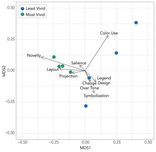
The nMDS plot of this data allowed for the visual analysis to see similarities and differences in the maps based on the vividness codes. On the nMDS plot (Figure 1), the points illustrated the maps in the set, and thus there are 242 points on the plot, one for each of the maps. Points closer to each other were those maps which had similar ratings on the vividness codes. Those that were farther apart from each other had more diversity in the ratings assigned based on the vividness codes. The vectors in the plot were the vividness attributes. The longer vectors were the vividness attributes which were more important in explaining the variance between the ratings of the maps.

Figure 1. nMDS plot of the maps produced by the top producers plotted based on the ratings of vividness.

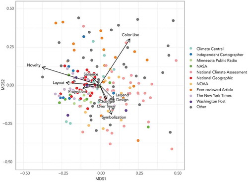
The primary attributes which accounted for more of the variance were: color use, novelty, and symbolization which had the longest vectors which can be identified visually. Vectors which pointed in the same direction illustrate the aspects which were more correlated. For instance, symbolization and change over time were correlated, but symbolization accounted for more of the variance noted by the length of the vector. Legend design and salience pointed in opposite directions which indicated that these attributes were not correlated, and neither accounted for very much of the variance in ratings.

There were three primary vectors in the nMDS plot: 1) color use; 2) novelty, layout, salience, and projection; 3) change over time, legend design, and symbolization. Color use, novelty, and symbolization dominated by accounting for a larger portion of the variance. It was rare that a map was rated highly on novelty, legend design, and color use. Points for maps at the center, instead, illustrated maps which had similar ratings across the aspects of vividness, but the nMDS plot does not illustrate whether the ratings were all high or all low.

When viewed in a matrix of small-multiple graphs, as in Figure 2, it was clear map producers focused on different aspects of vividness in their designs. In this case, there were clusters related to the producer. For instance, The New York Times and National Geographic maps clustered on the left-side of the plot, while the National Climate Assessment (produced by USGCRP) maps and NOAA maps were primarily located on the upper-right-side of the plots. This was because the maps at National Geographic and The New York Times used more novelty (an attribute which explained a large portion of the variance) such as 3D designs and interactivity. The National Climate Assessment and NOAA produced static single-variate maps which used color which aligned with connotations, and used understandable symbolization. In contrast, the “Other” category of maps were spread out across the space. This made sense, since being in the “Other” category, meant these maps were heterogeneous in both their producer and their designs.

Figure 2. Matrix of nMDS plots for each of the major producers who produced more than three maps. The longest vectors, or those which explain more of the variance, are labeled.

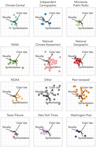
It was clear that vivid maps were often those designed in-house by media companies who knew more about their audiences than maps designed by government agencies whose maps were republished in a multitude of other outlets. For instance, NASA and NOAA published maps for their own audiences who tended to be the science-interested public, but these maps were also picked-up by many other media sources whose audiences differ. For instance, new digital media like Vox, Mashable, and Buzzfeed catered to a typically younger tech-savvy audience than NASA or NOAA’s general audience.

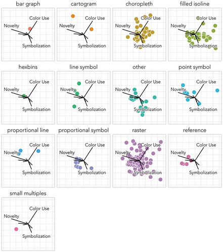
There were also patterns when comparing the use of dynamics (interactivity and animation) and the type of map design (Figures 3 and 4). Animated and interactive maps fell on the novel side of the graphic, while static maps were spread across the nMDS space. In Figure 4, it was clear that certain types of maps accounted for more of the maps in the sample. These were: choropleth, filled isoline, point symbol, proportional symbol, raster, and reference. Choropleth maps tended to be less novel and the points were primarily located on the right side of the nMDS space. Line symbol maps, on the other hand tended to be more novel as did some of the proportional symbol maps. Raster maps, perhaps because they accounted for most of the maps in the set, did not have any particular pattern in the nMDS space.

Figure 3. Matrix of nMDS plots by the use of dynamics. The longest vectors, or those which explain more of the variance, are labeled.

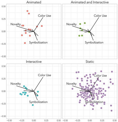
Figure 4. Matrix of nMDS plots for different map types. The longest vectors, those which explain most of the variance, are labeled.

5. Vivid map designs

The top four vivid maps were maps produced by The New York Times, National Geographic, and the Washington Post. To identify these maps, I summed the scores from the vividness coding. Three of these maps were static and only one was interactive. All of the maps told a story and could not simply be placed with different text and many contexts. I describe the commonalities between these maps here.

In the maps that did not include interactivity, the authors of the maps found ways to illustrate change over time and tell a story about changing landscapes and places through the maps. In “Mapping 50 Years of Melting Ice in Glacier National Park” the map illustrated change over time by removing all geographic context and simply showing the differences in glacial extents within the Park (Popovich, 2017). It did include a simple animated GIF at the top of the article too which showed how some of the more famous glaciers in the park have changed over time. According to the designer of the maps in this story, readers were perhaps fascinated by the removal of context. In an interview conducted as part of another study, she described this map “as something a little bit different” which might account for why we rated it as vivid and why the map was shared widely across several social media platforms (Fish, Under Review). In “The race to save Florida’s devastated coral reef from global warming” by the Washington Post the mix of high-resolution imagery with the color of the graduated symbols in red made the devastation to the reef clear even while it is not possible to actually see the devastation in the aerial image (Meko, 2017). The black background of this map as well as the “The Melting of Antarctica” map in National Geographic (Tierney et al., 2017) pushes all but the central map idea to the front of the visual hierarchy making this data salient against the background. This use of black background has become more common in recent years as more maps are published on the web but can still be considered novel. The “Antarctica” map also used an oblique view which presented this continent in a way that readers might feel like they are flying over this rapidly changing landscape. This map showed change through the use of arrows and line width, and it used colors which connected with reader connotations of melting ice.

The one map that used interactivity in these top four maps was a piece titled: “Alaska’s Permafrost is Thawing.” Published in The New York Times in August 2017 (White, 2017), this interactive/animated map used scrolling to juxtapose the extent of permafrost in 2010 with what could be lost in the future as the reader scrolled down the page. Many of the highly vivid maps across the sample (not only the top four) used this “scrolly-telling” to bring readers to places they may have never been and easily show transitions without asking readers to find and press buttons. Instead readers could simply scroll, an interaction that is easily used across a wide variety of devices. This design made this map novel since few other maps have employed this type of design. The cartographer limited what readers saw as they scrolled down the page and avoided overwhelming audiences by creating visual salience in each scene in the map. This map was simple enough that even a very novice user could engage and have fun. The map and article also incorporated photos which added to making the topic of climate change tangible for a general audience.

In summary, the maps which were vivid were those that followed cartographic best practices but also incorporated novel designs either through interactivity such as scrolly-telling or through the use of color, projection, or symbolization. In Figure 5, I illustrate where the top four most highly vivid maps and the lowest four rated maps were located in the nMDS space.

Figure 5. The nMDS plot indicates where the top four and lowest four maps are located in the nMDS space.

6. Conclusions

In this article, I reported on an empirical study which used content analysis to understand what media organizations produced and published maps of climate change, what topics were illustrated in their maps, and the extent to which these maps were vivid and which organizations produced vivid maps. I asked three questions for this study:

• (1) Which media organizations created and shared these maps and were they produced in-house or reproduced from other sources?

This research showed that the producers of maps of climate change are often not the publishers of this same content. Only a few sources produced their own maps for publication, primarily The New York Times and National Geographic. A majority of the maps were produced by government entities: NASA, NOAA, and the USGCRP. These maps were republished across a wide range of sources from prestige media to new digital media. In addition, maps from peer-reviewed articles also found their way to the media. These maps were often republished without any updates to the design and thus often were missing information key to the map reader’s understanding.

• (2) What aspects of climate change did these maps portray and what aspects of cartographic design did these maps employ?

These maps primarily showed topics which were relevant to audiences in the United States. Primarily these maps illustrated either the United States or the globe, and usually did not illustrate places outside the United States except the poles. Temperature was the most common topic (n = 51), followed by topics related to sea level rise, water resources, and glacial melt. The maps primarily were multicolored raster maps, although other types of thematic maps, such as choropleth and isoline were also common.

• (3) Did these maps convey climate change vividly and which organizations produced vivid maps?

Vividness is a concept from the communication literature and has been extended to the cartographic domain. Maps which were vivid were those which employed the eight aspects of vividness presented in this paper: legend design, symbolization, layout, projections which were appropriate for the data, visual salience, visible change over time, color use which aligned with color connotations, and novel design styles. Across the set of maps, most of the maps followed cartographic best practices, but less of the maps added novelty to stand out to readers. Primarily The New York Times, National Geographic, and The Washington Post created vivid maps by adding novelty which included the use of scrolly-telling and creating maps which were unusual in some way and were not simple output plots from climate models, statistical software, or GIS to make these maps memorable and stand out to readers.

6.1. Significance and future research

Identifying maps that have vivid attributes will allow for future research to evaluate the effectiveness of vivid maps for grabbing attention and persuading audiences. If these maps do indeed impact message effectiveness, as has been shown in other contexts (e.g. Guadagno et al., 2011), vivid map attributes will be those that can add to the wealth of cartographic principles we instill in new mapmakers. Vividness provided one way in which to identify those maps which did more than follow current cartographic conventions, expanding beyond those principles to bring the nature of geographic change to life through novelty, visible change over time, visual salience, and emotional uses of color. There have always been vivid maps, but like fashion, what is novel is ever-changing. What might be considered vivid now may be passé in the future. By evaluating maps in this way, cartographers now have a means by which to identify what types of maps are vivid or pallid for map readers. While this study focused specifically on climate change, future studies could extend this work beyond the domain of climate change to other contexts where maps have implications for translating knowledge to the public or for policymaking.

Future research could expand on some of the limitations of this study, specifically related to coding, and the presentation of the results of the nMDS. Future studies would be well served to have two coders who did not take part in the development of the coding scheme as has been suggested by Krippendorff (2013). In addition, I imagine another study building on this in which the coding is completed by expert cartographers in the form of a survey. While nMDS was an interesting and effective way in which to understand the differences in the vividness ratings for the maps, the presentation here in a static form has some limitations. Ideally, an interactive nMDS plot would allow users to mouse-over a point on the plot and see a visual of the associated map. This type of visual analytics may lead to some more interesting discoveries of patterns in this and other datasets.

In the set of maps, a few maps stood out as employing designs which were vivid in that these maps drew attention, brought climate change to life, made it tangible, evoked emotion, were memorable, and made climate change feel proximate in a temporal, sensory, or spatial way. These often were maps designed by elite media organizations, and not only followed cartographic conventions but incorporated novel designs like dynamic and interactive displays. This research leaves open questions about whether these maps are persuasive to readers, what types of design lead to greater sharing and re-sharing of these types of maps, and what aspects of the design and content lead to different emotional responses. Future research should test the effectiveness of vivid climate change maps, and expand the concept of cartographic vividness beyond the context of climate change.

Acknowledgments

The author would like to thank Cindy Brewer, Anthony Robinson, Roger Downs, and Janet Swim for feedback on an early draft of this paper. The author also wishes to thank Peter Ryan, Julia Higson, Nicole Rivera, and Han Yu for their assistance in data collection, and Peter Ryan for coding and assistance with R.

Data availability

The data that support the findings of this study are openly available in University of Oregon’s Scholars’ Bank at http://doi.10.7264/58x2-g466, URI: https://scholarsbank.uoregon.edu/xmlui/handle/1794/25303.

Disclosure statement

No potential conflict of interest was reported by the author.

Additional information

Funding

This research is based upon work supported by the National Science Foundation Doctoral Dissertation Research Improvement [Grant under Award No. 1735747]; National Center for Atmospheric Research, which is a major facility sponsored by the National Science Foundation under Cooperative Agreement [No. 1852977], and The Society of Woman Geographers Pruitt Fellowship.

References

- Abrams, L. (2014, May 6). 8 charts that show the terrifying reality of how climate change is affecting the U.S. Salon. https://www.salon.com/2014/05/06/8_charts_that_show_the_terrifying_reality_of_how_climate_change_is_affecting_the_u_s/
- Bertin, J. (1983). Semiology of graphics. University of Wisconsin Press. https://doi.org/10.2307/143508
- Boykoff, M. T., & Boykoff, J. M. (2007). Climate change and journalistic norms: A case-study of US mass-media coverage. Geoforum, 38(6), 1190–1204. https://doi.org/10.1016/j.geoforum.2007.01.008
- Chertoff, E. (2012, October 30). The sandy storm surge: Is this what climate change will look like? The Atlantic. https://www.theatlantic.com/technology/archive/2012/10/the-sandy-storm-surge-is-this-what-climate-change-will-look-like/264292/
- Chess, C., & Johnson, B. B. (2007). Information is not enough. In Susanne C. Moser & Lisa Dilling (Eds.), Creating a climate for change (pp. 223–233). Cambridge University Press. https://doi.org/10.1017/cbo9780511535871.017
- Dawson, B. (2013, February 10). A tale told in maps and charts: Texas in the national climate assessment. Texas Climate News. http://texasclimatenews.org/?p=6473
- DiBiase, D., MacEachren, A. M., Krygier, J. B., & Reeves, C. (1992). Animation and the role of map design in scientific visualization. Cartography and Geographic Information Science, 19(4), 201–214, 265–266. https://doi.org/10.1559/152304092783721295
- DiFrancesco, D. A., & Young, N. (2011). Seeing climate change: The visual construction of global warming in Canadian national print media. Cultural Geographies, 18(4), 517–536. https://doi.org/10.1177/1474474010382072
- Eaton, A. (2011). Unraveling the mystery of the elusive effect of vividness on persuasion. JOSHUA, 8, 56. https://pdfs.semanticscholar.org/ad10e41704eae54f4baaacf3f0518b6e3a643d4d.pdf#pag=56
- Fabrikant, S. I., Christophe, S., Papastefanou, G., & Maggi, S. (2012). Emotional response to map design aesthetics. 7th International Conference on Geographical Information Science (pp. 18–21). Springer. https://doi.org/10.5167/uzh-71701
- Fabrikant, S. I., & Goldsberry, K. (2005). Thematic relevance and perceptual salience of dynamic geovisualization displays. Proceedings, 22th ICA/ACI International Cartographic Conference, A Coruna. Spain. https://icaci.org/files/documents/ICC_proceedings/ICC2005/htm/pdf/oral/TEMA15/Session%203/SARA%20IRINA%20FABRIKANT.pdf
- Fish, C. S. (2020). Elements of vivid cartography. The Cartographic Journal. https://doi.org/10.1080/00087041.2020.1800160
- Griffin, A. L., & McQuoid, J. (2012). At the intersection of maps and emotion: The challenge of spatially representing experience. Kartographische Nachrichten, 62(6), 291–299. https://researchbank.rmit.edu.au/view/rmit:46588
- Guadagno, R. E., Rhoads, K. V. L., & Sagarin, B. J. (2011). Figural vividness and persuasion: Capturing the “elusive” vividness effect. Personality & Social Psychology Bulletin, 37(5), 626–638. https://doi.org/10.1177/0146167211399585
- Hannigan, J. (2014). Environmental sociology. Routledge.
- Hansen, J., Sato, M., & Ruedy, R. (2012). Perception of climate change. Proceedings of the National Academy of Sciences, 109(37), E2415–E2423. https://doi.org/10.1073/pnas.1205276109
- Harold, J., Lorenzoni, I., Shipley, T. F., & Coventry, K. R. (2016). Cognitive and psychological science insights to improve climate change data visualization. Nature Climate Change, 6(12), 1080–1089. https://doi.org/10.1038/nclimate3162
- Intergovernmental Panel on Climate Change [IPCC]. (2014). Climate Change 2014: Synthesis report. Contribution of working groups I, II and III to the fifth assessment report of the Intergovernmental Panel on Climate Change. IPCC. https://doi.org/10.1017/cbo9781107415416
- Joffe, H. (2008). The power of visual material: Persuasion, emotion and identification. Diogenes, 55(1), 84–93. https://doi.org/10.1177/0392192107087919
- Johannsen, I., Evers, M., & Fabrikant, S. I. (2018, April 11). What looks uncertain to you? An empirical study on how texture and color value communicate data quality in climate change maps. Annual Meeting of the American Association of Geographers. New Orleans, LA.
- Kaye, N. R., Hartley, A., & Hemming, D. (2012). Mapping the climate: Guidance on appropriate techniques to map climate variables and their uncertainty. Geoscientific Model Development, 5(1), 245–256. https://doi.org/10.5194/gmd-5-245-2012
- Kelley, C. A., Gaidis, W. C., & Reingen, P. H. (1989). The use of vivid stimuli to enhance comprehension of the content of product warning messages. Journal of Consumer Affairs, 23(2), 243–266. https://doi.org/10.1111/j.1745-6606.1989.tb00247.x
- Kessler, F. C., & Slocum, T. A. (2011). Analysis of thematic maps published in two geographical journals in the twentieth century. Annals of the Association of American Geographers, 101(2), 292–317. https://doi.org/10.1080/00045608.2010.544947
- Krippendorff, K. (2013). Content analysis: An introduction to its methodology. Sage.
- Landis, J. R., & Koch, G. G. (1977). An application of hierarchical kappa-type statistics in the assessment of majority agreement among multiple observers. Biometrics, 33(2), 363–374. https://doi.org/10.2307/2529786
- Lang, P. J., Greenwald, M. K., Bradley, M. M., & Hamm, A. O. (1993). Looking at pictures: Affective, facial, visceral, and behavioral reactions. Psychophysiology, 30(3), 261–273. https://doi.org/10.1111/j.1469-8986.1993.tb03352.x
- Manzo, K. (2012). Earthworks: The geopolitical visions of climate change cartoons. Political Geography, 31(8), 481–494. https://doi.org/10.1016/j.polgeo.2012.09.001
- Matthews, S. N., Iverson, L. R., & Prasad, A. M. (2009). 2007-ongoing. A climate change atlas for 147 bird species of the Eastern United States [database]. USDA/Forest Service. https://www.fs.fed.us/biology/main/wfw_newsletter/april_wfwnews_2009.pdf
- McCune, B., Grace, J. B., & Urban, D. L. (2002). Analysis of ecological communities (Vol. 28). MjM software design.
- McGill, A. L., & Anand, P. (1989). The effect of vivid attributes on the evaluation of alternatives: The role of differential attention and cognitive elaboration. Journal of Consumer Research, 16(2), 188–196. https://doi.org/10.1086/209207
- McKendry, J. E., & Machlis, G. E. (2008). Cartographic design and the quality of climate change maps. Climatic Change, 95(1–2), 219–230. https://doi.org/10.1007/s10584-008-9519-5
- Meko, T. (2017). The race to save Florida’s devastated coral reef from global warming [Map]. The Washington Post. https://www.washingtonpost.com/graphics/2017/business/environment/florida-reef/?utm_term=.55eab333f3af
- Moser, S. C. (2010). Communicating climate change: History, challenges, process and future directions. Wiley Interdisciplinary Reviews. Climate Change, 1(1), 31–53. https://doi.org/10.1002/wcc.11
- Muehlenhaus, I. (2011). Another Goode method: How to use quantitative content analysis to study variation in thematic map design. Cartographic Perspectives, 69(69), 7–30. https://doi.org/10.14714/cp69.28
- Muehlenhaus, I. (2012). If looks could kill: The impact of different rhetorical styles on persuasive geocommunication. The Cartographic Journal, 49(4), 361–375. https://doi.org/10.1179/1743277412Y.0000000032
- Muehlenhaus, I. (2013). The design and composition of persuasive maps. Cartography and Geographic Information Science, 40(5), 401–414. https://doi.org/10.1080/15230406.2013.783450
- Muehlenhaus, I. (2014). Going viral: The look of online persuasive maps. Cartographica: The International Journal for Geographic Information and Geovisualization, 49(1), 18–34. https://doi.org/10.3138/carto.49.1.1830
- Nerlich, B., Koteyko, N., & Brown, B. (2010). Theory and language of climate change communication. Wiley Interdisciplinary Reviews. Climate Change, 1(1), 97–110. https://doi.org/10.1002/wcc.2
- Nisbett, R. E., & Ross, L. (1980). Human inference: Strategies and shortcomings of social judgment. Prentice-Hall.
- O’Neill, S., & Nicholson-Cole, S. (2009). “Fear won’t do it” promoting positive engagement with climate change through visual and iconic representations. Science Communication, 30(3), 355–379. https://doi.org/10.1177/1075547008329201
- Otieno, C., Spada, H., Liebler, K., Ludemann, T., Deil, U., & Renkl, A. (2014). Informing about climate change and invasive species: How the presentation of information affects perception of risk, emotions, and learning. Environmental Education Research, 20(5), 612–638. https://doi.org/10.1080/13504622.2013.833589
- Popovich, N. (2017). Mapping 50 years of melting ice in glacier national park [Map]. The New York Times. https://www.nytimes.com/interactive/2017/05/24/climate/mapping-50-years-of-ice-loss-in-glacier-national-park.html
- Retchless, D. P. (2018). Understanding local sea level rise risk perceptions and the power of maps to change them: The effects of distance and doubt. Environment and Behavior, 50(5), 483–511. https://doi.org/10.1177/0013916517709043
- Retchless, D. P., & Brewer, C. A. (2016). Guidance for representing uncertainty on global temperature change maps. International Journal of Climatology, 36(3), 1143–1159. https://doi.org/10.1002/joc.4408
- Rose, G. (2012). Visual methodologies: An introduction to researching with visual materials (3rd ed.). Sage.
- Roth, R. E. (2013). An empirically-derived taxonomy of interaction primitives for interactive cartography and geovisualization. IEEE Transactions on Visualization and Computer Graphics, 19(12), 2356–2365. https://doi.org/10.1109/tvcg.2013.130
- Roth, R. E., Quinn, C., & Hart, D. (2015). The competitive analysis method for evaluating water level visualization tools. In J. Brus, A. Vondrakova, & V. Vozenilek (Eds.), Modern trends in cartography (pp. 241–256). Springer. http://link.springer.com/chapter/10.1007/978-3-319-07926-4_19
- Schultz, P. W. (2002). Empathizing with nature: The effects of perspective taking on concern for environmental issues. Journal of Social Issues, 56(3), 391–406. https://doi.org/10.1111/0022-4537.00174
- Shedler, J., & Manis, M. (1986). Can the availability heuristic explain vividness effects? Journal of Personality and Social Psychology, 51(1), 26. https://doi.org/10.1037//0022-3514.51.1.26
- Smith, N. W., & Joffe, H. (2009). Climate change in the British press: The role of the visual. Journal of Risk Research, 12(5), 647–663. https://doi.org/10.1080/13669870802586512
- Swim, J. K., & Bloodhart, B. (2015). Portraying the perils to polar bears: The role of empathic and objective perspective-taking toward animals in climate change communication. Environmental Communication, 9(4), 446–468. https://doi.org/10.1080/17524032.2014.987304
- Thompson, D. (2012, May 11). Our bad: Historic paper ties Texas droughts to human-caused climate change. The Atlantic. https://www.theatlantic.com/business/archive/2012/05/our-bad-historic-paper-ties-texas-droughts-to-human-caused-climate-change/257068/
- Tierney, L., Treat, J., & Tyson, S. (2017). The Melting of Antarctica [Map]. National Geographic.
- Tyner, J. A. (1982). Persuasive Cartography. Journal of Geography, 81(4), 140–144. https://doi.org/10.1080/00221348208980868
- U.S. Global Change Research Program. (2014). Climate change impacts in the United States: The third national climate assessment. U.S. Global Change Research Program. https://doi.org/10.7930/J0Z31WJ2
- Van der Linden, S. L., Leiserowitz, A. A., Feinberg, G. D., & Maibach, E. W. (2014). How to communicate the scientific consensus on climate change: Plain facts, pie charts or metaphors? Climatic Change, 126(1–2), 255–262. https://doi.org/10.1007/s10584-014-1190-4
- Weingart, P., Engels, A., & Pansegrau, P. (2000). Risks of communication: Discourses on climate change in science, politics, and the mass media. Public Understanding of Science, 9(3), 261–283. https://doi.org/10.1088/0963-6625/9/3/304
- White, J. (2017). Alaska’s permafrost is thawing [Map]. The New York Times. https://www.nytimes.com/interactive/2017/08/23/climate/alaska-permafrost-thawing.html
- Whitty, J. (2012, February 10). Climate change bird atlas. Mother Jones. https://www.motherjones.com/politics/2012/02/climate-change-bird-atlas/